Classical and Bayesian mixed model analysis of microarray data for detecting gene expression and DNA differences

(1)

2009

Classical and Bayesian mixed model analysis of

microarray data for detecting gene expression and

DNA differences

Cumhur Yusuf Demirkale

Iowa State University

Follow this and additional works at:

https://lib.dr.iastate.edu/etd

Part of the

Statistics and Probability Commons

This Dissertation is brought to you for free and open access by the Iowa State University Capstones, Theses and Dissertations at Iowa State University Digital Repository. It has been accepted for inclusion in Graduate Theses and Dissertations by an authorized administrator of Iowa State University Digital Repository. For more information, please [email protected].

Recommended Citation

Demirkale, Cumhur Yusuf, "Classical and Bayesian mixed model analysis of microarray data for detecting gene expression and DNA differences" (2009).Graduate Theses and Dissertations. 10760.

(2)

gene expression and DNA differences

by

Cumhur Yusuf Demirkale

A dissertation submitted to the graduate faculty in partial fulfillment of the requirements for the degree of

DOCTOR OF PHILOSOPHY

Major: Statistics

Program of Study Committee: Dan Nettleton, Co-major Professor Tapabrata Maiti, Co-major Professor

Alicia Carriquiry Heike Hofmann

Roger P. Wise

Iowa State University Ames, Iowa

2009

(3)

TABLE OF CONTENTS

LIST OF TABLES . . . v

LIST OF FIGURES . . . vii

ABSTRACT . . . ix

CHAPTER 1. General Introduction . . . 1

CHAPTER 2. Linear Mixed Model Selection for False Discovery Rate Con-trol in Microarray Data Analysis . . . 5

2.1 Introduction . . . 5

2.2 Example: Gene Expression in Barley . . . 8

2.2.1 Data . . . 9

2.2.2 Linear Mixed Model . . . 9

2.3 Candidate Analysis Methods . . . 11

2.3.1 Methods Involving Selection . . . 12

2.3.2 The ANOVA Approach . . . 13

2.4 Simulation Study . . . 14

2.4.1 Simulation Design . . . 14

2.4.2 Simulation Results . . . 15

2.5 Two-Stage Hybrid Method . . . 17

2.5.1 Description . . . 17

2.5.2 Application to Simulated data . . . 18

2.5.3 Application of the Hybrid Method to the Barley Data . . . 18

(4)

2.6.1 Assessing the Impact of Heavy-Tailed Errors . . . 20

2.6.2 Assessing the Impact of Missing Data . . . 20

2.7 Concluding Remarks . . . 21

2.8 References . . . 23

2.9 Appendix A: Model Selection . . . 24

2.9.1 BIC Formulation . . . 24

2.9.2 AIC and BIC for Model Selection . . . 24

2.10 Appendix B: Exact Inference Using ANOVA . . . 25

2.10.1 Mixed Linear Model . . . 25

2.10.2 ANOVA Construction of F-tests Based on Expected Mean Squares . . . 26

2.11 Appendix C: Tests for Main Effects . . . 33

2.11.1 The Test of Genotype Main Effects . . . 34

2.11.2 The Test of Time Main Effects . . . 36

2.12 Appendix D: Additional Simulation Studies . . . 38

2.12.1 Assessing the Impact of Percentage of Non-null Genes in the Data . . . 38

2.12.2 Assessing the Impact of Heavy-Tailed Errors . . . 39

2.12.3 Assessing the Impact of Missing Data . . . 39

CHAPTER 3. Bayesian Analysis of Microarray Experiments with Multiple Sources of Variation: A Mixed Model Approach . . . 71

3.2 Example: Gene Expression in Barley . . . 73

3.2.1 Data . . . 73

3.2.2 Linear Mixed Model Analysis of the Barley Data . . . 74

3.3 Bayesian Hierarchical Analysis . . . 76

3.3.1 Hierarchical Model . . . 76

3.3.2 Prior Specification . . . 77

3.3.3 Inference . . . 79

(5)

3.4.1 Simulation 1 . . . 82

3.4.2 Simulation 2 . . . 84

3.4.3 Simulation 3 . . . 86

3.5 Application of the Hierarchical Bayesian Method to the Barley Data . . . 87

CHAPTER 4. Identifying Single Feature Polymorphisms Using Affymetrix Gene Expression Data . . . 101

4.2 Background . . . 103

4.2.1 Affymetrix GeneChips . . . 103

4.2.2 Description of Single Feature Polymorphism . . . 104

4.3 Materials and Methods . . . 104

4.3.1 Data Sets . . . 104

4.3.2 Candidate Analysis Methods . . . 106

4.4 Application . . . 112

4.4.1 Identification of Single Feature Polymorphisms in Maize . . . 112

4.4.2 Identification of Single Feature Polymorphisms in Barley . . . 114

4.4.3 Identification of Single Feature Polymorphisms in the Soybean Data . . 116

CHAPTER 5. General Conclusion . . . 143

(6)

LIST OF TABLES

Table 2.1 AIC and BIC Selection for the Barley Data Set . . . 41

Table 2.2 Genotype-by-time Interaction Test: Results for the Complete Data . . 41

Table 2.3 Application of the Hybrid Method to the Barley Data Set . . . 42

Table 2.4 Genotype-by-time Interaction Test: Results for the Missing Data . . . 43

Table 2.5 AIC Selection for the Simulated Data with no Treatment Effect . . . . 44

Table 2.6 BIC selection for the Simulated Data with no Treatment Effect . . . . 44

Table 2.7 ANOVA Table . . . 45

Table 2.8 Genotype Test: Results for the Complete Data . . . 46

Table 2.9 Time Test: Results for the Complete Data . . . 47

Table 2.10 Genotype-by-time Interaction Test: Results for the Complete Data . . 48

Table 2.11 Genotype Test: Results for the Non-Normal Data . . . 49

Table 2.12 Time Test: Results for the Non-Normal Data . . . 50

Table 2.13 Genotype-by-time Interaction Test: Results for the Non-Normal Data . 51 Table 2.14 Genotype Test: Results for the Missing Data . . . 52

Table 2.15 Time Test: Results for the Missing Data . . . 53

Table 2.16 Genotype-by-time Interaction Test: Results for the Missing Data . . . 54

Table 3.1 MMA Results for the First Simulated Data . . . 91

Table 3.2 MMA and HBA results for the First Simulated Data . . . 91

Table 3.3 MMA Analysis Results for the Second Simulated Data . . . 92

Table 3.4 MMA and HBA results for the Second Simulated Data . . . 92

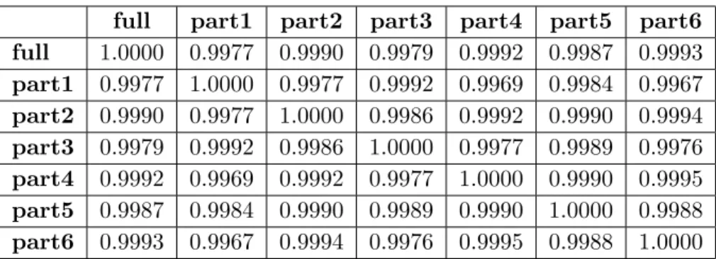
Table 3.5 Genotype Test: Correlations betweenF4 statistics . . . 93

(7)

Table 3.7 Genotype-by-time interaction Test: Correlations between F4 statistics 94

Table 3.8 Identifying Significant Genes in the Barley Data Set . . . 94 Table 4.1 SFP Identification by the Seven Method for the Five Tissues in the

Maize Data Set . . . 122 Table 4.2 SFP Identification by the Seven Method for the Six Tissues in the Barley

Data Set . . . 123 Table 4.3 Identifying SFPs in the Soybean Data Set . . . 124

(8)

LIST OF FIGURES

Figure 2.1 Genotype-by-time Interaction: Results for the Complete Data . . . 55

Figure 2.2 Genotype Test: Results for the Full Data Sets . . . 56

Figure 2.3 Time Test: Results for the Full Data Sets . . . 58

Figure 2.4 Genotype-by-time Interaction Test: Results for the Full Data Sets . . . 60

Figure 2.5 Genotype Test: Results for the non-normal Data . . . 62

Figure 2.6 Time Test: Results for the non-normal Data . . . 63

Figure 2.7 Genotype-by-time interaction Test: Results for the non-normal Data . 64 Figure 2.8 Genotype Test: Results for the Missing Data . . . 65

Figure 2.9 Time Test: Results for the Missing Data . . . 67

Figure 2.10 Genotype-by-time Interaction Test: Results for the Missing Data . . . 69

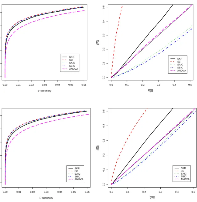
Figure 3.1 Genotype Test: ROC Curves for the First Simulated Data . . . 95

Figure 3.2 Time Test: ROC Curves for the First Simulated Data . . . 96

Figure 3.3 Genotype-by-Time Interaction Test: ROC Curves for the First Simu-lated Data . . . 97

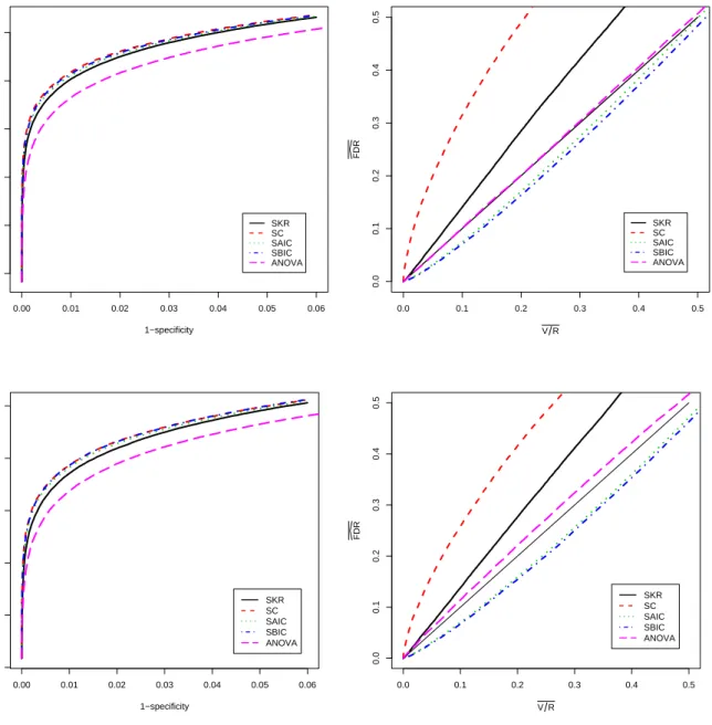
Figure 3.4 Genotype Test: ROC Curves for the Second Simulated Data . . . 98

Figure 3.5 Time Test: ROC Curves for the Second Simulated Data . . . 99

Figure 3.6 Genotype-by-Time Interaction Test: ROC Curves for the Second Sim-ulated Data . . . 100

Figure 4.1 Single Feature Polymorphisms Description . . . 125

Figure 4.2 Maize Data: Endosperm 19 DAP Tissue . . . 126

(9)

Figure 4.4 Maize Data: Immature Ear Tissue . . . 128

Figure 4.5 Maize Data: 19 DAP Embryo Tissue . . . 129

Figure 4.6 Maize Data: Seedling Tissue . . . 130

Figure 4.7 Barley Data: RAD Tissue . . . 131

Figure 4.8 Barley Data: COL Tissue . . . 132

Figure 4.9 Barley Data: CRO Tissue . . . 133

Figure 4.10 Barley Data: GEM Tissue . . . 134

Figure 4.11 Barley Data: LEA Tissue . . . 135

Figure 4.12 Barley Data: ROO Tissue . . . 136

Figure 4.13 Soybean Data: SFPs in Probe set Gma.734.1.A1 at . . . 137

Figure 4.14 Soybean Data: SFPs in Probe set Gma.11144.2.S1 at . . . 138

Figure 4.15 Soybean Data: SFPs in Probe set GmaAffx.39499.1.S1 at . . . 139

Figure 4.16 Soybean Data: SFPs in Probe set Gma.734.1.A1 at . . . 140

Figure 4.17 Soybean Data: SFPs in Probe set Gma.11144.2.S1 at . . . 141

(10)

ABSTRACT

This thesis focuses on classical and Bayesian mixed model analysis of microarray data for detecting gene expression and DNA differences. It consists of three research papers. The first study discusses the selection of gene specific linear mixed models in microarray data analysis. In a microarray experiment, one experimental design is used to obtain expression measures for all genes. One popular analysis method involves fitting the same linear mixed model for each gene, obtaining gene-specific p-values for tests of interest involving fixed effects, and then choosing a threshold for significance that is intended to control False Discovery Rate (FDR) at a desired level. When one or more random factors have zero variance components for some genes, the standard practice of fitting the same full linear mixed model for all genes can result in failure to control FDR. We propose a new method which combines results from the fit of full and selected linear mixed models to identify differentially expressed genes and provide FDR control at target levels when the true underlying random effects structure varies across genes. The second study discusses a hierarchical Bayesian modeling strategy for microarray data analysis. Some microarray experiments have complex experimental designs that call for mod-eling of multiple sources of variation through the inclusion of multiple random factors. While large amounts of data on thousands of genes are collected in these experiments, the sample size for each gene is usually small. Therefore, in a classical gene-by-gene mixed linear model analysis, there will be very few degrees of freedom to estimate the variance components of all random factors considered in the model and low statistical power for testing fixed effects of interest. To address these challenges, we propose a hierarchical Bayesian modeling strategy to account for important experimental factors and complex correlation structure among the expression measurements for each gene. We use half-Cauchy priors for the standard deviation

(11)

parameters of the random factors with few effects. We rank genes with respect to evidence of differential expression across the levels of a factor of interest by calculating a single sum-mary statistic per gene from the posterior distribution of the treatment effects considered in the model. Simulation shows that our hierarchical Bayesian approach is much better than a traditional gene-by-gene mixed linear model analysis at distinguishing differentially expressed genes from non-differentially expressed genes.

The third study focuses on the identification of Single Feature Polymorphisms (SFPs) using Affymetrix gene expression data. In microarray data analysis, the identification of SFPs is important for producing more accurate expression measurements when comparing samples of different genotypes. Also, portions of DNA that differ between parental lines can serve as markers for tracking DNA inheritance in offspring. We summarize several SFPs discovery methods in the literature. To identify single probes defining SFPs in the data, we developed two new algorithms where a difference value is defined for each probe after accounting for the overall gene expression level differences in the probe set. The first method contrast the difference value of each probe with the average of the difference values for the rest of the probes in that probe set. Second method is a robust version of the first method. The performance of all methods are compared through two publicly available published data sets, where truth about the sequence polymorphism is known for some “Gold Standard” probes. It was shown that our algorithms provided performance superior to the other methods in ordering probes for evidence of SFPs.

(12)

CHAPTER 1. General Introduction

Introduction:

Microarray technology has become an important tool in conducting biological research. It provides simultaneous measurements for the abundance of thousands of mRNA transcripts in multiple biological samples. These measurements are used to detect differentially expressed genes over different experimental conditions, time points, tissue samples, etc. Microarray ex-periments allow scientists to understand gene functions and learn how genes work together to carry out biological process. Based on the biological interest, microarray experiments are designed in various ways and based on the design, different statistical methods have been proposed for identifying differentially expressed genes. When the experiments have complex experimental designs that call for modeling of multiple sources of variation through the inclu-sion of multiple random factors, the use of linear mixed models is one of the common choice to make inference for each of thousands of genes. The motivation of this thesis is to provide improvement over analyses of microarray data that use linear mixed model for each gene.

In a microarray experiment, one experimental design is used to obtain expression measures for all genes. Traditional analysis method involves fitting the same linear mixed model for each gene, obtaining gene-specific p-values for the test of interest involving fixed effects and then choosing a threshold for significance that is intended to control False Discovery Rate (FDR) at a desired level. The primary focus in this analysis is the inference for fixed parameters. Such inference depends on the correct choice of random factors in each linear mixed model. Even though every gene shares the same experimental design, one or more random factors may affect the expression of only a subset of all measured genes. Then the standard practice of fitting the same full linear mixed model for all genes can result in failure to control FDR. Therefore

(13)

we propose a new method which combines results from the fit of full and selected linear mixed models to identify differentially expressed genes and provide FDR control at target levels when the true underlying random effects structure varies across genes.

Some biological problems require microarray experiments to have complex experimental de-signs. The linear mixed model need to include multiple random factor to account for multiple sources of variation. While large amounts of data on thousands of genes are collected in these experiments, the sample size for each gene is usually small. When a classical gene-by-gene mixed linear model analysis is conducted, there will be very few degrees of freedom to estimate the variance components of all random factors considered in the model and low statistical power for testing fixed effect(s) of interest. To address these challenges, it is common to use Bayesian models, which borrows strength across genes in estimating the gene specific parame-ters. One important requirement for this method to work properly is to choose the right prior distribution to account for the shared information between genes on the same array. We pro-pose a hierarchical Bayesian modeling strategy to account for important experimental factors and complex correlation structure among the expression measurements for each gene. Instead of classical prior choices for variance parameters, this model make use of the half-Cauchy priors for the standard deviation parameters of the random factors with few effects. We rank genes with respect to evidence of differential expression across the levels of a factor of interest by calculating a single summary statistic per gene from the posterior distribution of the fixed treatment effects considered in the model. We showed that our hierarchical Bayesian approach is much better than a traditional gene-by-gene mixed linear model analysis at distinguishing differentially expressed genes from non-differentially expressed genes.

In many microarray experiments, high-density oligonucleotide arrays are often used for measuring gene expression levels over different experimental conditions, time points, tissue samples. These arrays are also used for identifying possible DNA differences between genotypes, which include single nucleotide polymorphisms (SNPs) and insertion/deletions polymorphisms (IDPs) (Cui et al., 2005). Polymorphisms detected by a single probe in an oligonucleotide array are called a single-feature polymorphism (SFPs), where a feature refers to a probe in the array

(14)

(Borevitz et al., 2003). The identification of SFPs is important for producing more accurate expression measurements when comparing samples of different genotypes. Also, portions of DNA that differ between parental lines can serve as markers for tracking DNA inheritance in offspring. Therefore, there is need for new statistical methods to identify possible SFPs between genotypes. We address this problem by introducing two new statistical algorithms that make use of the linear mixed model analysis.

Finally, microarray experiments arise many challenging statistical problems, which moti-vates statistician to search for more appropriate methods in microarray data analysis. By this thesis, we provided an improvement over some current statistical analyses of microarray data that use the linear mixed models.

Thesis Organization:

This thesis consists of an introduction, three research papers, and a conclusion.

The second chapter is a paper accepted by Biometrics for publication. It focuses on se-lection of gene specific linear mixed models in microarray data analysis. The objective is to provide an improvement over analyses of microarray data that use the same linear mixed model for each gene. We proposed a two-step hybrid method for identifying differentially expressed genes with linear mixed model analysis. We have shown that our method provides better rank-ing with respect to evidence of differential expression across the levels of a factor of interest and FDR control at target levels. We used a barley microarray experiment as a motivating example.

The third chapter is an unpublished manuscript in which we present a hierarchical Bayesian modeling strategy for microarray data analysis. When the classical gene-by-gene linear mixed models cannot provide precise estimates of gene specific parameters due the small sample size for each gene, our hierarchical Bayesian model borrows strength across genes in estimating the gene specific parameters. We showed that with the right prior selection, the hierarchical Bayesian approach is much better than a traditional gene-by-gene mixed linear model analysis at distinguishing differentially expressed genes from non-differentially expressed genes.

(15)

identifica-tion of Single Feature Polymorphisms using Affymetrix gene expression data. In microarray data analysis, the identification of SFPs is important for producing more accurate expression measurements when comparing samples of different genotypes. We summarized several SFP discovery methods in the literature, and additionally, we introduced two new algorithms. The performances of all methods were compared through two publicly available published data sets, where truth about the sequence polymorphism is known for some “Gold Standard” probes. It was shown that our algorithms provided performance superior to the other methods in ordering probes for evidence of SFPs.

(16)

CHAPTER 2. Linear Mixed Model Selection for False Discovery Rate Control in Microarray Data Analysis

A paper accepted byBiometrics

Cumhur Yusuf Demirkale, Dan Nettleton, and Tapabrata Maiti

Abstract: In a microarray experiment, one experimental design is used to obtain expression measures for all genes. One popular analysis method involves fitting the same linear mixed model for each gene, obtaining gene-specificp-values for tests of interest involving fixed effects, and then choosing a threshold for significance that is intended to control False Discovery Rate (FDR) at a desired level. When one or more random factors have zero variance components for some genes, the standard practice of fitting the same full linear mixed model for all genes can result in failure to control FDR. We propose a new method which combines results from the fit of full and selected linear mixed models to identify differentially expressed genes and provide FDR control at target levels when the true underlying random effects structure varies across genes.

KEY WORDS: Analysis of variance; Method of moments; Multiple testing; Restricted maxi-mum likelihood; SAS; Variance component estimation.

2.1 Introduction

Microarray technology provides a means for simultaneously measuring the abundance of thousands of mRNA transcripts in multiple biological samples. These measurements are used to detect differentially expressed genes over different experimental conditions, time points,

(17)

tissue samples, etc. Many statistical methods for identifying differentially expressed genes have been proposed in the statistics literature in recent years.

One popular strategy involves conducting a linear mixed model analysis for each of thou-sands of genes. The basic approach was first proposed by Wolfinger et al. (2001) and has been applied in various forms by many researchers. The use of linear mixed modeling is convenient because such models allow for a natural and principled accounting for multiple sources of vari-ation. Because all the observations from a single microarray slide or chip share the same levels of all factors in a microarray experiment, the same experimental design applies to every gene. Thus, it is customary to fit the same linear mixed model for each gene. The common model is fit separately to the data from each gene to allow model parameters to be gene-specific. Tests for fixed effects of interest are carried out for each gene, and some correction for multiple testing is employed to help focus attention on the most relevant results.

False Discovery Rate (FDR) has become the most common error measure to control or estimate when declaring genes to be differentially expressed. FDR was first introduced by Benjamini and Hochberg (1995) and is formally defined asE(Q) where Qis the proportion of mistakenly rejected null hypotheses among all rejected null hypotheses or 0 if no hypotheses are rejected. Among many other approaches, Storey and Tibshirani’s (2003) method for FDR estimation has become a popular procedure that is less conservative than the original proposal of Benjamini and Hochberg.

When applying linear mixed models in microarray analysis, inference for the fixed param-eters is the primary focus. Such inference depends on the correct choice of random factors in each linear mixed model. Even though every gene shares the same experimental design, one or more random factors may affect the expression of only a subset of all measured genes. Thus, an analysis that fits the same linear mixed model for each gene may not provide correct fixed effect inferences, and it may be important to consider strategies for selecting the most appro-priate random factors on a gene-by-gene basis. Ideally, random factors with positive variance should be retained while those with zero variance components should be excluded. Tests for nonzero variance components could be used to identify relevant random factors. However,

(18)

available tests (e.g., Stram and Lee, 1994; Lin, 1997; Hall and Praestgaard, 2001) are only valid asymptotically. As the sample size for each gene is usually small, application of these tests to microarray data may be problematic.

A novel approach proposed by Chen and Dunson (2003) is to use a hierarchical Bayesian model for random-effects model selection, based on a decomposition of the covariance matrix of the random-effects distribution. The decomposition enables specification of a prior distribution that allocates positive probability to reduced models that exclude one or more random effects by setting their variances to zero. Although this method worked well for their simulated data, the application of this method to a simulated data set mimicking microarray data described in the next section was not successful, perhaps because of the limited per-gene sample sizes typical in microarray experiments. Additionally, this method is computationally intensive so that it is impractical to apply to each of thousands of genes in a microarray experiment.

Statistical analysts often use standard model selection measures such as Akaike’s informa-tion criterion (AIC) or Bayesian informainforma-tion criterion (BIC) to compare models with different random components. Although using AIC or BIC to choose random factors may be asymp-totically effective, application of these methods to analysis of a small data set for each gene from a microarray experiment may not be successful. In general for small data sets, these in-formation criteria unfortunately often fail to identify the correct covariance structure (Gomez et al. 2005). Furthermore, fixed effects testing following AIC or BIC model selection may not lead to valid inferences. In particular, we demonstrate in Section 2.4 that FDR controlling procedures can fail seriously when applied to p-values from tests of fixed effects from AIC- or BIC-selected linear mixed models.

In this paper, we propose a two-step hybrid method for identifying differentially expressed genes with linear mixed model analysis. Our method offers an improvement over analyses of microarray data that use the same linear mixed model for each gene. In the first step, we fit a full model for each gene based on the design of the experiment and produce a traditional ANOVA table. We construct F-tests for each fixed factor of interest based on appropriate ratios of mean squares to obtain a list of p-values (one for each gene) for any fixed factor of

(19)

interest. Each list ofp-values is used in conjunction with a standard FDR estimation procedure to find the number of genes to be declared as differentially expressed while controlling FDR at a specified level. In the second step, a gene-specific model is determined by using BIC to select the random part of the model among all random factors considered based on the design of the experiment. An hypothesis test of a fixed factor is performed by fitting the BIC favored model for each gene. Genes are ordered with respect to thep-values from this analysis. A target level false discovery rate is achieved for this list by declaring the same number of genes to be differentially expressed as identified in the first step. Therefore, the new method combines results from the fit of full and selected linear mixed models to identify differentially expressed genes and provides FDR control at target levels when the true underlying random effects structure varies across genes.

Our approach is motivated by several key observations that we note below and illustrate in subsequent sections of this paper. First, the traditional ANOVA analysis described above provides valid p-values as long as the true model is either the full linear mixed model or a reduced linear mixed model that contains a subset of the factors in the full model. Second, fixed effects inference following model selection is too liberal; i.e., estimated FDR levels tend to be much lower than the actual FDR. Third, although model selection prior to fixed effects inference leads to underestimation of FDR, the rank ordering of genes from most significant to least significant that is produced by model selection prior to testing is superior to the rank ordering produced by the traditional ANOVA analysis. Taken together, these observations imply that our procedure will be superior to a traditional full-model ANOVA analysis with regard to identification of differentially expressed genes but will also control FDR. Thus, our procedure maintains the most desirable features of full-model ANOVA analysis and analysis following model selection.

2.2 Example: Gene Expression in Barley

Caldo, Nettleton and Wise (2004) conducted a microarray experiment to identify barley genes that play a role in resistance to a fungal pathogen. To illustrate our methods, we describe

(20)

the analysis of a subset of the data they considered.

2.2.1 Data

Two genotypes of barley seedlings, one resistant and one susceptible to a fungal pathogen, were grown in separate trays randomly positioned in a growth chamber. Each tray contained six rows of 15 seedings each. The six rows in each tray were randomly assigned to six tissue collection times: 0, 8, 16, 20, 24, and 32 hours after fungal inoculation. After simultaneously inoculating plants with the pathogen, each row of plants was harvested at its randomly assigned time. One Affymetrix GeneChip was used to measure gene expression in the plant material from a pool of the 15 seedlings in each row. The entire process was independently repeated a total of three times, yielding data on 22,840 probe sets (corresponding to barley genes) for each of the 36 GeneChips (two genotypes ×six time points ×three replications). The actual

experiment involved a third barley genotype as well as a second infection type, but we focus on the reduced data set here to simplify the presentation of our main ideas. The expression levels in the reduced data were log-transformed and median centered before an analysis was performed.

2.2.2 Linear Mixed Model

The design of the experiment can be viewed as a split-plot with replications as blocks, trays as whole plots and rows of seedlings within trays as split plots. Note that although time is a factor in this experiment, this is not a repeated-measures design because no one plant or pool of plants is measured at multiple time points. Instead, because the measurement process is destructive, different randomly selected plants are sampled at each time. Therefore the following linear mixed model corresponding to the split-plot design was considered as a base model for each gene. Let

Yijk=µ+γj+τk+θjk+αi+βij+δik+ǫijk (2.1)

(21)

where Yijk is the observed intensity of a gene at the kth harvesting time for the jth genotype

during theith replication,γj is the fixed genotype effect, τk is the fixed tissue collection time

effect, θjk is the genotype-by-time interaction effect, αi ∼N ID(0, σ2α) is the random

replica-tion effect,βij ∼N ID(0, σβ2) is the replication-by-genotype interaction effect (corresponding to

trays) , δik ∼N ID(0, σδ2) is the replication-by-time interaction effect, and ǫijk ∼N ID(0, σ2ǫ)

is the error (N ID=Normally and Independently Distributed). Though not standard for a split-plot design, the replication-by-time interaction effects were included to account for the possibility of variation across harvest events; one random effect was included for each combi-nation of replication and time so that the two observations for the two samples (one of each genotype) collected at any one time in any one replication were allowed to be correlated due to the shared replication-by-time random effect. All the random effects are assumed to be jointly independently distributed and to be independent of the residual errors.

For each gene, this linear mixed model was fit to the 36 log-scale measures of expression using the SAS PROC MIXED procedure. Scientists were interested in identifying barley genes that play a role in resistance to the fungal pathogen. Such genes were expected to show patterns of expression over time that differed between the two genotypes. Therefore, the hypothesis test for interaction between genotype and time was considered to be of primary importance for each linear mixed model analysis, though tests for genotype main effects and time main effects were conducted also. Restricted Maximum Likelihood (REML) was used to estimate the variance components, and the Kenward-Roger (KR) method (Kenward and Roger, 1997) was used to determine the denominator degrees of freedom and F-statistics for tests of fixed effects. Applying the method of Storey and Tibshirani (2003) to obtain nominal control of FDR at 1% yielded a total of 399, 13202, and 93 genes for the tests of genotype, time, and interaction effects, respectively.

For each of the 22,840 genes, SAS PROC MIXED also produced REML estimates of the three variance components corresponding to three random factors. The variance component estimate for replication, replication-by-genotype, and replication-by-time was reported as zero for a total of 8153, 7824, and 7235 genes, respectively. For these genes, SAS PROC MIXED

(22)

with KR adjustment automatically fits a reduced model that excludes random factors whose variance component estimates are zero. Thus, this common analysis strategy employs an implicit gene-specific model selection step where random factors are selected for the model if and only if their variance component estimates are positive. Considering the full model or a reduced model may alter the result of any fixed-effect test substantially. In Section 4, we investigate the impact of this and other model selection strategies on tests for fixed-effects inference in linear mixed model analysis of microarray data when correct random structure varies from gene to gene.

2.3 Candidate Analysis Methods

In this section, we describe five methods for conducting gene-by-gene linear mixed model analysis of our microarray data set. Our list of methods is, of course, not exhaustive. However, we have included what we believe are the five most obvious choices, and it is easy to generalize our final recommendation to incorporate other strategies. We first list the five methods and then provide some additional explanation of the methods before comparing them in a simulation study in Section 4.

1. SKR: REML estimation of variance components with the KR method for conducting fixed-effects inference.

2. SC: REML estimation of variance components with SAS’s containment method for con-ducting fixed-effects inference.

3. SAIC: Selection of random factors according to Akaike’s Information Criterion (AIC) followed by analysis of the selected model using REML estimation of variance components with the KR method for conducting fixed-effects inference.

4. SBIC: Selection of random factors according to Schwarz’s Bayesian Information Criterion (BIC) followed by analysis of the selected model using REML estimation of variance components with the KR method for conducting fixed-effects inference.

(23)

5. ANOVA: Full model fitting using the method of moments to estimate variance compo-nents andF-test construction based on expected mean squares.

Note that, for our experimental design and tests, methods 1, 2, and 5 produce identicalp-values when all REML variance component estimates are positive. All five methods produce identical p-values when all REML variance component estimates are positive and AIC and BIC each select the full model.

2.3.1 Methods Involving Selection

The first four methods have abbreviations that begin with S to indicate that some form of model selection is employed. If there are q random factors, 2q _{candidate models can be}

considered. According to the experimental design of the barley data set described in Section 2.1, three random factors were considered in the full model for each gene. Therefore we can choose the best model for each gene among 23_{= 8 models. For the SKR and SC approaches, the}

model selection is simply carried out by removing random factors whose variance components are estimated to be zero. The SKR approach was described in Section 2.2.2. The SC approach differs from SKR in that the denominator degrees of freedom used for testing genotype, time, and genotype-by-time interaction are held constant at their full model values of 2, 10, and 10, respectively, regardless of which variance components are estimated to be zero.

The SAIC and SBIC approaches use the standard model selection measures AIC and BIC to choose random factors. For each of these models, AIC and BIC are calculated by SAS PROC MIXED as

AIC =−2l+ 2d and BIC =−2l+dlog(n),

respectively, wherelis the maximized log-likelihood (ML) or maximized restricted log-likelihood (REML),dis the total number of parameters in the model (ML) or number of parameters in the covariance structure (REML), andnequals the number of levels of the first random factor specified in the model. A model with smaller AIC or BIC is considered to be better. We used the total number of observations per gene (36 in our data set) asnwhen using BIC to compare models with different random factors. We argue in Appendix A that this is preferable to the

(24)

SAS default which depends on the order that factors are listed in the RANDOM statement and can lead to obviously poor model choices when leading factors have zero variance component estimates.

Eight models were fitted for each of 22,840 genes in the barley data set. AIC and BIC were used to select random factors for each gene. The number of models favored by AIC and BIC are reported in Table 2.1. For example, for 4277 genes, AIC chose a model whose random part consisted of the replication random factor only, whereas BIC favored this same model for 3787 genes. Gomez et al. (2005) conducted a simulation study regarding the performance of AIC and BIC in selecting the true covariance structure from a large set of repeated-measures covariance structures. In Appendix A, we examine the effectiveness of AIC and BIC covariance selection in the context of our linear mixed model and present findings similar to those of Gomez et al. (2005).

2.3.2 The ANOVA Approach

The ANOVA approach involves no model selection. The full model is fit to every gene regardless of variance component estimates or information criteria. The classical analysis of variance (ANOVA) table is used to construct F-tests for the fixed effects of interest. The test statistic for testing each fixed factor is defined by

F = SSF F/df1 SSRF/df2

, (2.2)

where SSF F and df1 are the sum of square and degrees of freedom with respect to a fixed

factor of interest, respectively, and SSRF and df2 are the sum of squares for the random

factor corresponding to the experimental units of the fixed factor and its degrees of freedom, respectively. The expected mean squares E(SSF F/df1) and E(SSRF/df2) are identical when

the null hypothesis is true. Under the standard linear mixed model assumptions outlined previously, the test statistic follows an F-distribution under the null hypothesis, even if one or more true variance components are zero. Details for our model and tests are provided in

Web Appendix B. These ANOVA-basedF-tests are easily obtained with SAS PROC MIXED

(25)

2.4 Simulation Study

The power and type I error properties of tests of fixed-effects following random factor selection are generally unknown and analytically intractable. Nonetheless, some type of data-dependent model selection – either formal or informal – is commonly used by data analysts when fitting linear mixed models to individual data sets. Because microarray data analysis involves thousands of such analyses, the impact of model selection on inferential properties can be dramatic. In this section, we describe a large data-driven simulation study designed to examine the performance of the methods described in Section 2.3.

2.4.1 Simulation Design

Fifty data sets, each containing 22,840 genes, were generated from versions of the linear mixed model (1) described in Section 2.2.2. When simulating the data sets, we mimicked the original barley data by generating a random effects structure for each gene that matched the random effects structure of the model selected by AIC for that gene (see Table 2.1). The selected random effects were sampled independently from normal distributions with mean zero and variance equal to the variance component estimate of the corresponding random factor. Genotype, time, and genotype-by-time interaction effects were set to zero for 90% of the genes in each data set. For the other 10% of the genes in each data set, the observed gene-specific means for each combination of genotype and time in the original barley data were added to the normally distributed mean-zero random effects to create non-null genotype, time, and genotype-by-time interaction effects for these genes.

The five methods described in Section 2.3 were used to analyze each of the 50 data sets. One set of 22,840 p-values was produced for each combination of data set, method, and test (genotype, time, or interaction) for a total of over 17 million p-values. More than 9 million linear mixed model analyses were conducted because the SAIC and SBIC methods required that 8 models be fit to each data set and gene. Each set of 22,840 p-values was converted to q-values using the method of Storey and Tibshirani (2003), and these q-values were used to produce estimates of FDR for any significance threshold.

(26)

2.4.2 Simulation Results

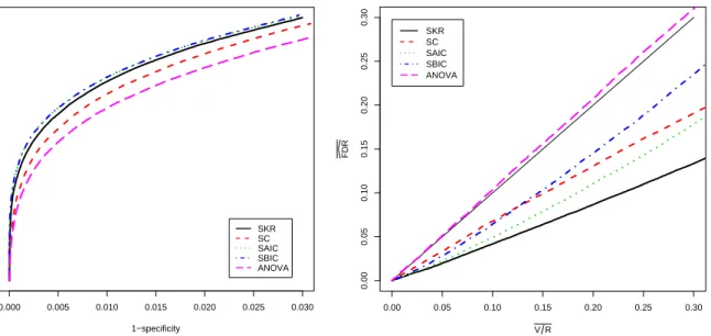
In this section, we describe the performance of our methods for the test of genotype-by-time interaction which is of primary interest in our application. Analogous results, including tables and figures, are presented for the test of genotype main effects and time main effects in Appendix C. For the test of interaction, we begin with an examination of receiver oper-ator characteristic (ROC) curves to compare the effectiveness of the methods for separating differentially and non-differentially expressed genes. The p-values produced by each method provide a rank order of genes from most evidence for differential expression to least evidence. The quality of the ranking varies from method to method and can be judged by comparing ROC curves. The greater the area under an ROC curve the better the corresponding method is at distinguishing null genes from non-null genes. The left panel of Figure 2.12.3 shows ROC curves for the five methods averaged over the 50 simulated data sets. The patterns of the curves and differences among the curves were quite similar for each simulation run so little in-formation is lost by averaging. Differences among the curves are statistically significant except for the SAIC and SBIC comparison. For example, pointwise standard errors are approximately 0.001 or less at 1−specificity values of 0.005, 0.015, and 0.025; and simple sign tests for

pair-wise differences between the curves at these 1−specificity values yield significance at below the

0.000001 level for all comparisons except SAIC vs. SBIC. Note also that we have plotted the curves over only the most informative ranges of sensitivity and 1−specificity. The left panel of

the figure shows that an analysis with AIC or BIC selected models is slightly more effective at distinguishing non-null from null genes than the SKR approach. The SC approach lags behind the SKR approach, and the ANOVA method is least effective.

The ability to correctly rank genes with regard to evidence for differential expression is clearly important because the goal of our analysis is to identify differentially expressed genes. However, the effectiveness of a method at ranking genes is not the only important measure of performance. Good statistical procedures include an accurate assessment of the degree of uncertainty associated with an analysis. In microarray analysis, it is common to produce a list of differentially expressed genes and an estimated false discovery rate. The number of genes

(27)

placed on the list is often determined by the FDR level that a researcher is willing to tolerate. Thus, we now investigate the FDR control properties of our five methods.

Using notation from the seminal FDR paper by Benjamini and Hochberg (1995), we let V = the number of type I errors when the R tests with the smallestp-values are declared to be non-null. Separately for each set of p-values, we recorded the actual false positive fraction (V /R) and the estimated FDR level (FDR given by thed q-value for theRth_{gene) for all values}

of R from 1 to 22,840. We averaged the results for each method over the 50 data sets to obtain the right panel of Figure 2.12.3. Again, the results for individual data sets were quite consistent so that no important information was lost by averaging.

Ideally, the plotted curves would fall on or above the diagonal reference line to indicate that the actual average false positive fraction (V /R) was no larger than the average estimated FDR level. For all methods that involve some form of model selection, the estimated curves fell substantially below the reference line. This indicates a clear problem with FDR control for these methods. In contrast, the ANOVA approach produced FDR estimates that were on average very close to the actual average false positive fraction. This is expected because the ANOVA-based F-tests have the correct size as discussed in Appendix B.

The top portion of Table 2.2 further illustrates the error control properties of our proce-dures. For each of the 50 data sets and each of the five methods discussed in Section 3, the approach of Storey and Tibshirani (2003) was used to generate lists of significant genes for nominal FDR control at the 0.01 and 0.05 levels. The number of genes on each list and the number of false positives on each list was recorded. The averageV /Rfraction and the average number of genes on the list across the 50 data sets were computed. Although the ANOVA ap-proach identified the fewest genes on average, it was the only procedure that provided control of FDR at or below nominal levels. Note that the SKR and SAIC approaches had estimated FDR levels (V /R) more than twice the nominal rate. Although not presented in Table 2.2, for each of the 50 data sets, the false positive fraction was always higher than the nominal FDR levels (0.01 and 0.05) for the first four methods in the Table 2.2.

(28)

five analysis methods, the one that is least effective at distinguishing null from non-null tests (ANOVA) is the only approach that appropriately controls type I error rate for each individual test and the FDR for a family of tests. In the next section, we discuss a hybrid procedure that combines the positive attributes of the testing procedures into a single approach that provides good power for distinguishing null and non-null tests while controlling FDR.

2.5 Two-Stage Hybrid Method

2.5.1 Description

We propose a hybrid method which combines results from the fit of full and selected linear mixed models to identify differentially expressed genes and provide FDR control at target levels when the true underlying random effects structure varies across genes. The two-step procedure can be described as follows:

1. For each gene, perform the ANOVAF-test of fixed effects. For any test of a fixed factor of interest, estimate FDR by using the method of Storey and Tibshirani (2003) or any other method with similar FDR controlling properties. For a desired level of FDR, determine D= the number of genes to be declared as differentially expressed.

2. Forq possible random factors in the design of the experiment, fit all 2q _{possible models}

for each gene. Find the model with the lowest AIC or BIC value for each gene and obtain the p-value for the test of interest from that model. Declare the D genes with the D smallest p-values to be differentially expressed, where Dis as determined in step 1. Because both the AIC- and BIC-selected models better distinguish null and non-null genes than the ANOVA approach, this hybrid method will have lower FDR and better power than the ANOVA approach. Because the ANOVA approach appropriately controls FDR, the hybrid will also control FDR – albeit at lower levels than nominal. We demonstrate these properties via simulation in the next subsection.

(29)

2.5.2 Application to Simulated data

To illustrate the performance of the hybrid method in identifying differentially expressed genes and providing FDR control at or below target levels, 50 microarray data sets were generated. As described in Section 2.4, in each data set, the true underlying random effects structure varied across genes, and the data for 10% of the genes were simulated with non-zero genotype, time, and interaction effects.

We applied the hybrid method using AIC model selection in step 2 and also using BIC model selection in step 2. We also considered the hybrid approach where the full model fit with the KR method and containment method were used in step 2 rather than either of the formal model selection approaches. These methods are referred to as ANOVA-SAIC, ANOVA-SBIC, ANOVA-SKR, and ANOVA-SC, respectively, in the results presented below. For brevity, we report the results only for the test of interaction between genotype and time. Similar results for the test of genotype and time are discussed in Appendix C.

As for the methods of Section 2.3, we calculated the length of the significant gene list and the true false positive fraction (V /R) associated with each of the gene lists for each data set and averaged over the 50 data sets. The results are presented in the lower portion of Table 2.2. By comparison with the top portion of Table 2.2, we can see that each of the two-step hybrid methods improved on the ANOVA approach by providing smaller false positive fractions than the ANOVA approach. In practice, the hybrid approach will identify the same number of genes as ANOVA but will tend to include more genes that are truly differentially expressed than ANOVA alone. Though our simulation results show that all the hybrid methods provided FDR control at better than nominal levels, ANOVA-SAIC and ANOVA-SBIC outperformed ANOVA-SKR and, especially, ANOVA-SC. Thus, we recommend either ANOVA-SAIC or ANOVA-SBIC in practice.

2.5.3 Application of the Hybrid Method to the Barley Data

Scientists were interested in identifying barley genes that play a role in resistance to a fungal pathogen. Such genes are believed to have patterns of expression over time following

(30)

infection that differ between susceptible and resistant genotypes. Therefore, we are particularly interested in identifying genes that exhibit interaction between genotype and time.

Table 2.3 shows the number of genes identified as differentially expressed at nominal FDR levels of 0.01 and 0.05 using each of the nine methods that we have studied in this paper. The gene lists produced by the recommended methods ANOVA-SAIC and ANOVA-SBIC differed from each other by 2 and 23 genes at nominal FDR of 0.01 and 0.05, respectively, and differed from the pure ANOVA approach by 17 and 86 genes (ANOVA-SAIC) and 15 and 89 genes (ANOVA-SBIC). Either the ANOVA-SAIC gene lists or the ANOVA-SBIC gene lists would be appropriate to use in practice. Although the first four methods in Table 2.3 provided longer gene lists, the simulations in Section 2.4 suggest that FDR levels will be higher than nominal for these procedures.

2.6 Performance when ANOVA Tests are Not Exact

Although our proposed method is versatile and can be applied to data from many complex experimental designs, the approach is not guaranteed to perform well when ANOVA-based F-tests are not exact. An approximateF-test will not necessarily control type I error rates at nominal levels, especially when sample sizes are small. If the type I error rate of an individual test is not controlled, the usual FDR controlling procedures will fail in the multiple hypothesis testing setting.

In practice, there are several situations in which ANOVA-based F-tests may fail to be ex-act. Missing data or the presence of outlying observations are two related problems commonly encountered in microarray analysis that can lead to non-exact tests. Due to the technological challenges of measuring the expression of thousands of genes simultaneously in multiple sam-ples, some outlying observations are inevitable. If such observations are included as part of the data set, the error distribution tends to be heavy-tailed for at least some genes, and the usual assumption of normally distributed errors becomes questionable. As an alternative, some data analysts favor strategies that involve automated outlier detection and removal. The impact of these often ad hoc strategies on the inferential properties of subsequent tests is unknown and

(31)

cannot be studied here. However, we have conducted additional simulation studies to assess the effect of either heavy-tailed errors or missing data on our proposed analysis strategies.

2.6.1 Assessing the Impact of Heavy-Tailed Errors

The simulation study described in Subsection 2.4.1 was repeated using scaledt-distributed errors rather than normal errors. For each gene, the ǫijk terms in model (1) were obtained

by drawing 36 independent observations from a t distribution with five degrees of freedom. These observations were then multiplied by the gene-specific error standard deviation that was estimated from the original barley data. Other than a decrease in power for all methods, the results were essentially the same as those discussed in Sections 2.4 and 2.5. In particular, for the interaction test, the ANOVA approach controlled FDR at the 0.01 and 0.05 levels, the methods involving selection were too liberal, and the hybrid approaches ANOVA-SAIC and ANOVA-SBIC performed best overall. The complete results – including figures and tables for the tests of genotype main effects, time main effects, and interaction – are provided in Appendix D.

2.6.2 Assessing the Impact of Missing Data

Imbalance in data due to missing observations can make some ANOVA F-tests non-exact. In our case, the test for interaction between genotype and time remains exact when data are missing completely at random. In contrast, the ANOVA F-tests for genotype and time main effects become only approximate (unless data remain balanced following the loss of a complete replication). To study the effect of imbalance caused by missing data on ANOVA-based mixed linear model analyses, we conducted two new variations of the simulation study described in Subsection 4.1. In the first version, three entire gene chips were randomly selected and removed from the data set so that all genes were missing three of their 36 observations. In the second version, four genotype-by-time combinations were randomly selected and two of the three observations for each selected combination were randomly selected for removal from the data set. This process was done separately for each gene. Thus, in the second version of the

(32)

simulation study, a random eight of the 36 observations were missing for each gene.

Table 2.4 presents results for the test of interaction between genotype and time when data are missing. By comparison with Table 2.2, it is clear that all methods suffered a decrease in power as the proportion of missing data increased. Also, the failure of the SKR, SAIC, and SBIC methods to control FDR worsened as the proportion of missing data increased. In contrast, the liberal bias of the SC method – although still clearly evident at the nominal 5% level – was reduced by missing data. The ANOVA method and all hybrid approaches continued to control FDR at or below nominal levels. As in the case of no missing data, the ANOVA-SAIC and ANOVA-SBIC methods provided the best performance among methods that controlled FDR. However, note that when eight of the 36 observations were missing for each gene, the ANOVA and hybrid approaches had almost no power to identify differentially expressed genes. This is not surprising given that nearly one fourth of each data set was missing and only two error degrees of freedom were available for nearly half the genes. Although the ANOVA tests for genotype and time main effects defined in (2.2) are no longer exact when data are missing, control of FDR below nominal levels was obtained for both of our missing data scenarios. Complete results for the tests of genotype and time main effects are provided in Appendix D.

2.7 Concluding Remarks

We have focused on the specific problem of using linear mixed model analyses of microarray data to control the false discovery rate when identifying differentially expressed genes. Our main idea applies in greater generality. Consider any multiple hypothesis testing problem involvingN tests where FDR control is desired. Consider two procedures (denotedP1 andP2)

for ranking the tests from most evidence against the null hypothesis to least evidence. Suppose that it is possible to determine R1 = the number of tests according toP1 to declare non-null

so that FDR will be controlled at level α. By definition of FDR, this means that

(33)

where Vk(r) denotes the number of true null hypotheses among the top r tests as ranked by

procedurePk. Suppose that

E[V1(r)]≥E[V2(r)] for allr= 1, . . . , N . (2.4)

It is straightforward to show that (2.3) and (2.4) imply E[V2(R1)/(R1∨1)]≤α. Thus, using

procedure P1 to determine the number of null hypotheses to reject while using procedure P2

to determinewhichnull hypotheses to reject will control FDR and provide fewer type 2 errors on average than using procedure P1 alone. In our case, we can choose ANOVA and SAIC (or

SBIC) approaches asP1 andP2, respectively, to obtain the desired performance characteristics

as illustrated through simulation in Section 2.4.

Although we have focused on obtaining correct fixed-effects inference rather than necessarily identifying the correct random-effects model, correct inference and correct model selection are undeniably connected. Tables 2.5 and 2.6 are contingency tables that give counts for each combination of true and selected model for AIC and BIC selection, respectively, for one simulated example data set. Both AIC and BIC selected the correct model for slightly more than 50% of the genes (52.5% for AIC and 52.8% for BIC). This performance is typical and consistent with the findings of Gomez et al. (2005). It is likely that other model selection strategies (e.g., corrected AIC, Hurvich and Tsai, 1989) could improve the probability of correct selection, but such methods will undoubtedly suffer from the type I error control problems that we have documented for AIC and BIC selection.

Based on our simulation results in Sections 2.4 through 2.6, it is clear that our hybrid procedure can be quite conservative in that actual FDR levels may be far below nominal. This situation results because the operator characteristics of testing following model selection are far superior to those of the ANOVA method alone. We are of the traditional opinion that an error rate below nominal is preferred to an error rate above nominal. The ability to produce error rates no larger than nominal is one hallmark of a good statistical testing procedure and a feature that distinguishes statistical approaches from other approaches that offer decisions without assessments of the uncertainty associated with those decisions. Nonetheless, there is room to improve the power of our proposed procedures, and we hope to address this issue in

(34)

future research.

2.8 References

Benjamini, Y., and Hochberg,Y. (1995). Controlling the false discovery Rate: a Practical and Powerful Approach to Multiple Testing. Journal of the Royal Statistical Society, Series B, 57, 289-300.

Caldo, R. A., Nettleton, D., Wise, R. P. (2004). Interaction-dependent gene expression in Mla-specified response to barley powdery mildew. The Plant Cell., 16, 2514-2528.

Chen, Z., and Dunson, D.B.(2003). Random effects selection in linear mixed models. Biometrics,

59, 762-769.

Gomez, E.V., Schaalje, G.B., and Fellingham, G.W. (2005). Performance of the Kenward-Roger method when the covariance structure is selected using AIC and BIC.Communications in Statistics — Simulation and Computation, 34, 377-392.

Hall, D.B. and Praestgaard, J.T. (2001). Order-restricted score tests for homogeneity in generalized linear and non-linear mixed models. Biometrika, 88, 739-751.

Hurvich, C.M. and Tsai, C.-L. (1989). Regression and time series model selection in small samples. Biometrika,76, 297-307.

Kenward, M. G. and Roger, J. H. (1997). Small sample inference for fixed effects from restricted likelihood. Biometrics, 53, 983-997.

Lin, X. (1997). Variance component testing in generalized linear models with random effects.

Biometrika, 84, 309-326.

Storey, J.D., and Tibshirani, R. (2003). Statistical significance for genomewide studies. Proc. Natl. Acad. Sci. USA,100, 9440-9445.

Stram, D.O. and Lee, J.W. (1994). Variance components testing in the longitudinal mixed effects model. Biometrics,50, 1171-1177.

(35)

Wolfinger, R., Gibson, G.,Wolfinger, E., Bennett, L., Hamadeh, H., Bushel, P., Afshari, C., and Paules, R. (2001). Assessing Gene Significance from cDNA Microarray Expression Data via Mixed Models. Journal of Computational Biology,8, 625-637.

2.9 Appendix A: Model Selection

2.9.1 BIC Formulation

Selection of the preferred model using BIC as computed by SAS can be problematic when some variance components are estimated to be zero. For example, assume that a full mixed linear model includingd random factors is fit to a data set. Suppose the variance component of the first random factor is estimated to be zero while all other variance components are estimated to be positive. Then PROC MIXED will automatically fit a reduced model that excludes the first random factor. SAS will correctly use d−1 as the number of parameters

in the REML likelihood but will inappropriately use the number of levels of the first random factor as n in BIC calculation even though this factor has been excluded from the model. If we manually fit the reduced model by omitting the first random factor, all results are identical to the results from the full model fit except that the number of levels of the second random factor in the full model will be used asn in BIC calculation. If the number of levels of second random factor is greater than the number of levels of the first random factor, the BIC that SAS calculate for the full model will be lower than the BIC that SAS calculates for the reduced model even though requesting the full model fit in SAS actually results in the reduced model fit. An algorithm that would fit all 2dmixed models would favor the full model over the reduced model which excludes the first random factor even though there is no evidence to support the more complicated model. To avoid this problem, we calculated BIC using the total number of observations per gene (36 in our data set) asnin the BIC formula.

2.9.2 AIC and BIC for Model Selection

We conducted a simulation study to explore AIC and BIC covariance selection in the setup of the barley data design. A data set, containing 22,840 genes, was generated by following

(36)

the method described in Section 2.4. Eight models were fit for each of 22,840 genes, and AIC and BIC were each used to select a model for each gene. Both AIC and BIC selected the correct model for slightly more than 50% of the genes (52.5% for AIC and 52.8% for BIC). The following supplementary Tables 2.5 and 2.6 are contingency tables that give counts for each combination of true and selected model for AIC and BIC selection, respectively.

2.10 Appendix B: Exact Inference Using ANOVA

2.10.1 Mixed Linear Model

Consider the mixed linear model described in Section 2.2.2

Yijk=µ+γj+τk+θjk+αi+βij+δik+ǫijk (2.5)

i= 1,2,3;j = 1,2;k= 1, . . . ,6. where

• Yijk is the observed intensity of a gene at the kth harvesting time for the jth genotype

during theith replication,

• γj is the fixed genotype effect,

• τk is the fixed tissue collection time,

• θjk is the genotype-by-time interaction,

• αi is the random replication effect, assume αi ∼N ID(0, σ2α),

• βij is the replication-by-genotype interaction, assumeβij ∼N ID(0, σ_β2),

• δik is the replication-by-time interaction, assumeδik∼N ID(0, σδ2), and

• ǫijk∼N ID(0, σ2ǫ) is the error.

(37)

Σ =        V 0 0 0 V 0 0 0 V        V =    (σ 2 δ+σ2ǫ)I+ (σα2 +σβ2)J σδ2I+σ2αJ σ2 δI+σα2J (σδ2+σ2ǫ)I+ (σ2α+σβ2)J    • whereI is the 6×6 identity matrix and

• J equals the 6×6 matrix containing only ones.

2.10.2 ANOVA Construction of F-tests Based on Expected Mean Squares

For testing fixed effects, we can construct F tests from the ANOVA table (Table 2.7) by taking the ratio of mean squares. For example, the F-statistic for testing the fixed genotype effect is the ratio of the mean square for genotype and the mean square for replication-by-genotype. Under the standard mixed linear model assumptions outlined previously, this test statistic follows an F distribution even if the underlying true model for this gene is different from the full model. As an illustration, for three cases (underlying true models), we will show that this is true. For other models, the same argument follows.

1. Assume that full model was the true model for the data, i.e., σ2

α > 0, σ2β > 0, and

σ_δ2 >0.

• Hypothesis Test for fixed genotype effect: _{The null hypothesis is}

H0:γ1+ 1 K X k θ1k=γ2+ 1 K X k θ2k (2.6)

and based on the ANOVA table above, the test statistic is the ratio of two mean squares such that F1 = M Sgeno M Srep−geno = IK P j(Y.j.−Y...)2/(J−1) KP_iP_j(Yij.−Yi..−Y.j.+Y...)2/(I−1)(J−1) = Y T_A 1Y /(J−1) YT_A 2Y /(I−1)(J −1) (2.7)

(38)

where A1 = ₃₆1                   J −J J −J J −J −J J −J J −J J J −J J −J J −J −J J −J J −J J J −J J −J J −J −J J −J J −J J                   , A2 = ₃₆1                   2J −2J −J J −J J −2J 2J J −J J −J −J J 2J −2J −J J J −J −2J 2J J −J −J J −J J 2J −2J J −J J −J −2J 2J                   and A1A1 =A1,A2A2 =A2,A1A2 = 0. A1Σ = (σ2ǫ + 6σ2β)A1 andA2Σ = (σǫ2+ 6σβ2)A2 Then YT_A 1Y /(σǫ2+ 6σβ2)∼χ2(J−1) and YTA2Y /(σǫ2+ 6σβ2)∼χ2(I−1)(J−1) and

A1ΣA2 = (σǫ2+ 6σβ2)A1A2= 0. Hence YTA1Y and YTA2Y are independent.

Hence,F1∼F(J−1),(I−1)(J−1).

• Hypothesis Test for fixed time effect: _{The null hypothesis is,}

H0:τ1+ 1 J X j θj1=τ2+ 1 J X j θj2=. . .=τK+ 1 J X j θK1 (2.8)

and based on the ANOVA table, the test statistic is expressed as, F2 = M Stime M Srep−time = IJ P k(Y..k−Y..)2/(K−1) IP_jP_k(Y.jk−Y.j.−Y..k+Y...)2/(I−1)(K−1)

(39)

= Y T_A 3Y /(K−1) YT_A 4Y /(I−1)(K−1) (2.9) where A3 = ₃₆1        6I−J · · · 6I−J .. . . .. ... 6I−J · · · 6I−J        and A4 = ₃₆1                   2(6I−J) 2(6I−J) −(6I−J) −(6I−J) −(6I−J) −(6I−J) 2(6I−J) 2(6I−J) −(6I−J) −(6I−J) −(6I−J) −(6I−J) −(6I−J) −(6I−J) 2(6I−J) 2(6I−J) −(6I−J) −(6I−J) −(6I−J) −(6I−J) 2(6I−J) 2(6I−J) −(6I−J) −(6I−J) −(6I−J) −(6I−J) −(6I−J) −(6I−J) 2(6I−J) 2(6I−J) −(6I−J) −(6I−J) −(6I−J) −(6I−J) 2(6I−J) 2(6I−J)                   and A3A3 =A3,A4A4 =A4, andA3A4 = 0. A3Σ = (σ2ǫ + 2σ2δ)A3 and A4Σ = (σǫ2+ 2σδ2)A4 Then YT_A 3Y /(σǫ2+ 2σδ2)∼χ2(K−1) and YTA4Y /(σ2ǫ + 2σδ2)∼χ2(I−1)(K−1) and

A3ΣA4 = (σǫ2+ 2σδ2)A3A4 = 0. HenceYTA3Y and YTA4Y are independent.

Hence,F2∼F(K−1),(I−1)(K−1).

• Hypothesis Test for the interaction between genotype and time:

The null hypothesis is,

(40)

and based on the ANOVA table, the test statistic follows as, F3 = M Sgeno−time M SE = IPjPk(Y.jk−Y.j.−Y..k+Y...)2/(J−1)(K−1) M SE = Y T_A 5Y /(J −1)(K−1) YT_A 6Y /(I−1)(J−1)(K−1) (2.11) where A5 = ₃₆1                   (6I−J) −(6I−J) (6I−J) −(6I−J) (6I−J) −(6I−J) −(6I−J) (6I−J) −(6I−J) (6I−J) −(6I−J) (6I−J) (6I−J) −(6I−J) (6I−J) −(6I−J) (6I−J) −(6I−J) −(6I−J) (6I−J) −(6I−J) (6I−J) −(6I−J) (6I−J) (6I−J) −(6I−J) (6I−J) −(6I−J) (6I−J) −(6I−J) −(6I−J) (6I−J) −(6I−J) (6I−J) −(6I−J) (6I−J)                   and A6 = 1 36                   2(6I−J) −2(6I−J) −(6I−J) (6I −J) −(6I−J) (6I−J) −2(6I−J) 2(6I−J) (6I−J) −(6I −J) (6I−J) −(6I−J) −(6I−J) (6I−J) 2(6I−J) −2(6I −J) −(6I−J) (6I−J) (6I−J) −(6I−J) −2(6I−J) 2(6I −J) (6I−J) −(6I−J) −(6I−J) (6I−J) −(6I−J) (6I −J) 2(6I−J) −2(6I−J) (6I−J) −(6I−J) (6I−J) −(6I −J) −2(6I−J) 2(6I−J)                   and A5A5 =A5,A6A6 =A6,A5A6 = 0. A5Σ =σǫ2A5 and A6Σ =σǫ2A6

Then YTA5Y /σ2ǫ ∼χ2(J−1)(K−1) and YTA6Y /σ2ǫ ∼χ2(I−1)(J−1)(K−1) and

A5ΣA6 =σ2ǫA5A6 = 0. Hence YTA5Y andYTA6Y are independent.

Hence,F3∼F(J−1)(K−1),(I−1)(J−1)(K−1).

2. Assume that none of the random effects is present in the model, i.e., σ2

α = 0, σβ2 = 0, and

(41)

The full model from (1) will reduce to

Yijk=µ+γj+τk+θjk+ǫijk

and the variance-covariance matrix will be,

Σ1 =σ2ǫI

whereI is the 36×36 identity matrix.

• Hypothesis Test for fixed genotype effect: _{The null hypothesis is the same as}

(2) and the test statistic is the same as (3). It is sufficient to show A1 (σ2 ǫ + 6σ2β) Σ1 = A1 σ2 ǫ σ_ǫ2I =A1, A2 (σ2 ǫ + 6σ2β) Σ1 = A2 σ2 ǫ σ_ǫ2I =A2,

and A1 andA2 are idempotent. Then,

YT_A

1Y /(σ2ǫ + 6σ2β)∼χ2(J−1) and YTA2Y /(σǫ2+ 6σ2β)∼χ2(I−1)(J−1) and

A1Σ1A2 =σ2ǫA1A2 = 0. Hence YTA1Y andYTA2Y are independent.

Hence,F1∼F(J−1),(I−1)(J−1).

• Hypothesis Test for fixed time effect: _{The null hypothesis is the same as (4)}

and the test statistic is the same as (5). It is sufficient to show A3 (σ2 ǫ + 2σδ2) Σ1= A3 σ2 ǫ σ2_ǫI =A3, A4 (σ2 ǫ + 2σδ2) Σ1= A4 σ2 ǫ σ2ǫI =A4,

(42)

YT_A

3Y /(σ2ǫ + 2σ2δ)∼χ2(K−1) and YTA4Y /(σǫ2+ 2σδ2)∼χ2(I−1)(K−1) and

Hence,F2∼F(K−1),(I−1)(K−1).

• Hypothesis Test for the interaction between genotype and time: _{The null}

hypothesis is the same as (6) and the test statistic is the same as (7). It is sufficient to show A5 σ2 ǫ Σ1= A5 σ2 ǫ σ_ǫ2I =A5, A6 σ2 ǫ Σ1= A6 σ2 ǫ σ_ǫ2I =A6,

YT_A

5Y /σǫ2∼χ2(J−1)(K−1) and YTA6Y /σǫ2∼χ2(I−1)(J−1)(K−1) and

Hence,F3∼F(J−1)(K−1),(I−1)(J−1)(K−1).

3. Assume that replication and replication-by-genotype random effects are present in the model but no replication-by-time, i.e., σ2

α >0,σβ2 >0, andσδ2= 0.

The full model from (1) will reduce to

Yijk =µ+γj+τk+θjk+αi+βij+ǫijk

and the variance-covariance matrix will be,

Σ5 =        V5 0 0 0 V5 0 0 0 V5       

(43)

V5 =    σ 2 ǫI+ (σ2α+σβ2)J σ2αJ σα2J σ2ǫI+ (σ2α+σβ2)J   

• Hypothesis Test for fixed genotype effect: _{The null hypothesis is the same as}