The Extent of Volatility Predictability Evaluation of forecasting accuracy dependent on time, distribution and model order

(1)

The Extent of Volatility Predictability

Evaluation of forecasting accuracy dependent on time, distribution and model order

Authors

Robert Dadson and Marta Slonka

Supervisor

Valeriy Zakamulin

This master’s thesis is carried out as a part of the education at the University of Agder and is therefore

approved as a part of this education. However, this does not imply that the University answers for the methods that are used or the conclusions that are drawn.

University of Agder, May 2015 School of Business and Law Department of Economics and Finance

(2)

Abstract

This thesis focuses on the accuracy and ability of out-of-sample volatility forecasting over different time horizons. Using data at daily frequency we forecast the future volatility over multiple time horizons (1, 3, 6, 9 and 12 months) and evaluate the goodness of forecasting by comparing the Naïve, ARCH, GARCH, EGARCH and GJR-GARCH models using the MSE and the Predictive Power (P). We include different probability distributions for the error terms in an attempt to improve the models accuracy. The research is conducted using three indices: FTSE 100, S&P 500 and the Hang Seng. We find that the goodness of forecasting accuracy decreases dramatically after the 3 month horizon and the selection of a more representative error distribution improves the accuracy of the short term forecasts. The results also show that the higher order GARCH models, beyond (1,1), do not improve the forecasting accuracy.

(3)

1. Introduction

Volatility forecasting is of known importance for risk management, portfolio optimization and option pricing through its contribution to the measurement of potential future losses. Volatility is the uncertainty of asset prices over a given investment time horizon. When forecasted well the investor or financial institution is able to assess the investment risk accurately and achieve a level of risk they are willing to accept. The information provided by volatility is indispensible and was recognised in 2003 with the Nobel Memorial Prize in Economic Sciences being shared by Robert F. Engle and Clive Granger. In his prize lecture at the University of Stockholm, Engle went on to say:

“There are some risks we choose to take because the benefits from taking them exceed the possible costs. Optimal behaviour takes risks that are worthwhile. This is

the central paradigm of finance; we must take risks to achieve rewards but not all risks are equally rewarded. Both the risks and the rewards are in the future, so it is the

expectation of loss that is balanced against the expectation of reward. Thus we optimize our behaviour, and in particular our portfolio, to maximize rewards and

minimize risks”(Engle (2003))

Volatility is estimated from historical data on asset returns while implied volatility uses observed option prices which, from a theoretical perspective, are a good estimate of future realized volatility as they include all relevant and available information. Investors and financial institutions use volatility as a key input in risk management models when forecasting. Much research has been devoted to modelling and forecasting the volatility of financial returns where the modelling of volatility for asset pricing purposes relies on the accurate assessment of future returns and risk. Model risk, as discussed in Figlewski (1998), suggests that there exits a risk that any given model may be misspecified. It is of necessity, when modelling, to specify the stochastic process of the underlying asset. Most existing papers use the log-normal process assumed by the original option-pricing model of Black and Scholes (1973), whereas the empirically correct distribution of the actual financial markets under analysis are likely to be non-normal. This thesis directly compares three different error distributions in order to overcome the difficulty in the judgment of the accuracy

(5)

of such models. Empirical finance literature has shown that volatility series develop over time in non-linear fashion due to the mean reverting properties of the models. We investigate the performance of volatility forecasting within the class of Autoregressive Conditional Hetroskedastic (ARCH) models due to their capability of capturing the non-linear features of financial time series and the possibility of extending these models to consider additional features.

The Autoregressive Conditional Hetroskedasticity (ARCH) model introduced by Engle (1982) was one of the first models that provided a way to model conditional hetroskedasticity in volatility. Bollerslev (1986) extended the ARCH model to the Generalized Autoregressive Conditional Hetroskedasticity (GARCH), which has the same basic properties as the ARCH model but requires far less parameters to satisfactorily model the volatility process. Both the ARCH and GARCH models are able to model the persistence and clustering of volatility but are unable to distinguish between the different influences that positive and negative shocks have on the volatility. To be able to model this behaviour and overcome the weaknesses of the ARCH and GARCH models, Nelson (1991) proposed an extension to the GARCH model called the Exponential GARCH (EGARCH), which is capable of taking into account the asymmetric effects of positive and negative asset returns. An additional extension of the GARCH model is the GJR-GARCH which was proposed by Glosten, Jagannathan and Runkle (1993).

The purpose of this thesis is to analyze the methods of forecasting volatility over long term horizons, the longest being 12 months, and compare the results with shorter forecasting time horizons. This thesis adds to the existing literature in several ways. First of all, we examine the importance of assumptions regarding the distributions of the error term. Previous studies have shown that the normal error distribution, which is widely applied in the majority of research, does not necessarily fit the models, nor give the most accurate forecasts (Speight, McMillan and Gwilym (2000)). Thus, in this thesis, three different error distributions are applied (Normal, Student t and Generalized Error Distribution). Secondly, we use various (from 1 month up to 12 months) forecasting horizons. There exist only a few papers that cover longer than 3 months forecasting periods because in practice, variability in volatility is often used in

(6)

horizons are thus of interest to those who, for example, try to find the correct price for financial instruments such as long-term options (called LEAPS - Long-term Equity Anticipation Securities), or warrants which mostly have an expiration of up to 1 year but in some countries up to 3 years. Much of the existing research only covers one time horizon and therefore the comparison of results directly between different indices and time horizons is difficult to establish.

Forecasting the future level of volatility over any horizon is far from straightforward and evaluating the forecasting performance presents an additional challenge. The majority of the 93 papers reviewed by Poon and Granger (2003) use the Mean Squared Error (MSE), or the Root Mean Squared Error (RMSE), which uses the actual and forecasted volatilities to compare the differences. Our third difference is that we also assess the Predictive Power (P) in order to find out how much of the future variability in volatility our models are able to predict. We do this by calculating the proportion of explained variability as proposed by Blair, Poon and Taylor (2010). The comparison of forecasting models for indices from three different continents is also rare since the majority of exists papers focus on multiple markets of individual countries. We have chosen to study the following three indices, FTSE 100, S&P 500 and Hang Seng.

We find that the level of forecasting accuracy decreases as the time horizon increases. The forecasting horizon which produces the most accurate statistics is that of 1 month for the FTSE 100 and S&P 500, and 3 months for the Hang Seng index. The GARCH models with a larger number of properties were found to be better predictors than the more restrictive models and higher order models beyond (1,1) do not significantly improve the accuracy. With the use of three different error distributions we generally see an improvement in accuracy when using the two non-normal distributions compared to that of the Gaussian distribution when considering shorter forecasting horizons.

The rest of the thesis is organized as follows. In Section 2, we review relevant literature and familiarize the reader with the existing research papers regarding volatility forecasting over long term horizons, as well as those that cover similar models and error distributions. In Section 3 we examine the characteristics of the data and analyze the descriptive statistics of the returns. Furthermore, we investigate the

(7)

distributions and continue with graphs and statistics of the realized monthly volatility. In Section 4 we describe the methodology for each model including how the forecasts are performed and the three error distributions used. We also explain how the models are going to be compared. In Section 5 we present and interpret the results of each index. The models are presented individually based on the shortest to longest forecast horizon. We then, in Section 6, discuss the important findings and contrast our results with those of literature reviewed. Section 7 provides a concise summary of our approach and main findings.

2. Literature review

The majority of the papers regarding volatility forecasting study the predictability over horizons shorter than 3 months (usually 1 month). Moreover, the model selection varies where not one individual model is preferred over others. Even when empirical work uses the same models and markets, the observations and evaluation methods differ, thus, the conclusions rarely agree. In this thesis we focus on the length of horizon predictability using the ARCH/GARCH family models whilst considering the model's sensitivity to distribution assumptions and time horizons. Below we review some relevant papers regarding these matters.

Poon and Granger (2003) make a review of papers regarding volatility forecasting. They compare 93 papers under various models, distributions and forecasting horizons. The review is clear evidence that researchers mostly prefer to forecast volatility for short time horizons yet there are a few relevant papers which focus on longer horizons and these are revealed below.

Scott and Tucker (1989) study the predictive accuracy of standard deviations and the constant elasticity of variance (CEV) implied in American currency call options traded on the Philadelphia Stock Exchange (PHLX). Five currencies are used, namely the British pound, Canadian dollar, German deutschmark, Japanese yen, and the Swiss franc. The authors accumulate daily closing prices and forecast subsequent currency return volatility for 3, 6 and 9 months. The obtained forecasting results are evaluated using the MSE. The authors conclude that the MSEs are statistically

(8)

indistinguishable and suggest that the simple Black-Scholes predictions are as good as those achieved from the CEV model.

Kroner, Kneafsey and Claessens (1995), using daily data, derive long-term horizon (225 calendar days ahead) forecasts of various commodity price volatilities. The authors use seven models to forecast volatility (ISD (Implied Standard Deviation), ISDAT (ISD from the at-the-money option), ISDAVG (weighted average of ISDs), HV (historical volatility), GARCH, COMB (which combines the ISD and GARCH forecasts) and GR (Granger and Ramanathan regression weighted combined forecast)). The results are compared by means of the MSE and ME. The two combined methods, namely GR and COMB, are found to give the most accurate predictions and outperform other forecasts.

Figlewski (1997) collects results from his earlier research papers regarding volatility forecasting for option pricing applications and investigates long-term horizon volatility forecasting using daily and monthly historical data. The most relevant for our thesis is where he investigates the long-term (1, 3, 6, 12, 24 months) forecasting accuracy of Historical Volatility (HV) and GARCH models by means of the RMSE. He finds the GARCH (1,1) model to be the best at forecasting volatility for the S&P 500 index over all time horizons, but in all other markets (3M US Bill, 20Y T-Bond, Deutschemark Exchange Rate (DM per $)) its performance is very poor.

Green and Figlewski (1999), forecast volatility of the S&P 500 stock index, 3-month LIBOR (short-term interest rate), 10-year T-Bond yield (long-term interest rate) and DM exchange rate, by means of HV and Exponential Smoothing (ES). While using daily data, the forecast horizon varies from 1 to 12 month. Comparing RMSE, the authors find that ES is a better tool than HV for the short term S&P 500 (1–3 months) and the LIBOR, while bond yield, exchange rate and long-term S&P 500 (12 months) volatility are forecasted more accurately by means of the HV. They do importantly note that when the forecasted horizon is expanded the estimation period should also be expanded, in order to give reasonable long-term forecasts. In the second part of their studies they lengthen the forecast horizon to 2 and 5 years, and use monthly instead of daily data. In this case the HV outperforms ES for all four underlying assets.

(9)

Ederington and Guan (2002) wrote a paper in which they investigate whether the implied volatility is an informationally efficient and effective predictor of future volatility. The interesting aspect for us is in regards to the accuracy of the applied models (Implied Volatility, GARCH (1,1) and HV). In this study they use daily data for options on S&P 500 futures and forecast volatility of overlapping option maturity for 7-90, 91-180, 181-365 and 7-365 days ahead. The authors show that GARCH (1,1) outperforms the HV but at the same time it performs worse than the Implied Volatility. Additionally their findings confirm, as per the properties of the model, that the volatility forecasted by GARCH tends to converge to a constant at longer horizons.

Li (2002), uses Implied Volatility and the Autoregressive Fractionally Integrated Moving Average (ARFIMA) model to forecast volatility of forward options on 3 different currencies, for 1, 2, 3 and 6 months. The five-minute and daily returns on the German deutschemark, the Japanese yen, and the British pound vs. the US dollar are used. The Mean Absolute Error (MAE) reveals that the Implied Volatility provides more an accurate prediction at shorter time horizons while ARFIMA is more suitable for longer forecasts.

Since we compare four ARCH/GARCH models there is an additional aspect in Poon and Granger (2003), which we are interested in, namely, the analysis of 17 studies, which compare alternative versions of ARCH and GARCH models and their ability to forecast. The authors remark that, most of the time, papers use different data frequencies and do not explicitly suggest a clear rank of the models, thus it is difficult to point to an ultimate “winner”. They are however able to come to a main conclusion that GARCH models tend to outperform the more restrictive ARCH model.

Cao and Tsay (1992) use stock market data at daily and monthly frequencies to test which of the following models: Threshold Autoregressive (TAR), Autoregressive–

Moving-Average model ARMA (1,1), ARCH (1,1) and EGARCH (1,0), give the most accurate volatility forecasts. They compare the forecasting ability over multiple horizons (from 1 to 30 months) by means of the MSE and MAE. The most relevant

(10)

finding is that the EGARCH (1,0) model gives the best volatility forecasts over long-time horizons, which they suggest is due to the leverage effect1_.

The use of different distribution assumptions in existing empirical works is rather poor, yet we review two papers which investigate this issue. Liu and Morley (2009), research whether forecasts based on the GARCH family models can outperform simple historical averaging models. In their paper, they use nine different models and apply daily and weekly sample frequencies. The authors test the forecasts sensitivity by applying three different error distributions (Normal, Student-t and Generalized Error Distribution). They reveal that the volatility forecasting is indeed sensitive to the assumption made about the use of different error distribution statistics. Moreover, they show that whilst not all of the models give better outcomes than the simple historical averaging, the use of non-normal distributions in the application of GARCH models, fits the in-sample data better and gives a better one-period ahead volatility forecast than the more commonly used normal distribution.

In the master thesis by Wei (2012), the author predicts the conditional variance of the rate of return in five different markets, including three used in this thesis, in terms of daily data. Three different forecasting models are applied, namely: GARCH (1,1), E-GARCH (1,1) and GJR-E-GARCH (1,1) (2,1) (1,2) (2,2). By means of these models, the author studies forecasting performance under two different error distributions (Normal and Student t-distribution) and reports their accuracy with the use of the RMSE over a forecasting horizon of 1 year. The results exhibit that the normal distribution improves the models and the higher order GJR-GARCH outperforms other models in all cases except for the Hang Seng Index, where the GARCH (1,1) with a normal error distribution has the smallest RMSE.

1_{The leverage effect is generally a negative correlation between the return of an asset and its changes}

(11)

3. Data Analysis

3.1 Indices

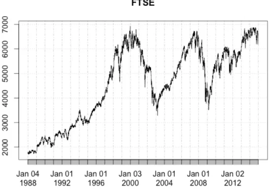
The Financial Times Stock Exchange (FTSE) 100 index is a market capitalization-weighted index of United Kingdom-listed blue chip2_{companies and is the most}

widely used UK stock market indicator. The index was launched on the 3rd_{of January}

1984 with a base date of the 30th_{December 1983 and a base value of 1000. The FTSE}

100 measures the performance of the 100 largest companies, which are traded on the London Stock Exchange, and represents 81% of the entire market capitalization. The index is part of the FTSE UK Series and was designed for use in the creation of index tracking funds, derivatives and also as a performance benchmark. The top 5 constituents are HSBC Holdings, Royal Dutch Shell, BP Oil & Gas, GlaxoSmithKline Pharmaceuticals & Biotechnology and British American Tobacco .

Figure 1: FTSE 100 index 1988-2014.

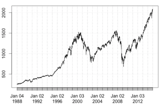
The Standard and Poor (S&P) 500 (also referred to as GSPC) is a capitalization-weighted index composed of the 500 leading companies listed on the New York Stock

(12)

Exchange and NASDAQ. The index was established on the 4th_{of March 1957 and}

was the first American based market capitalization-weighted stock index. Nowadays, the S&P 500 captures about 80% coverage of available market capitalization and is the basis of numerous listed and over-the-counter investment instruments. The S&P 500 was intended to measure performance of the domestic economy through changes in the aggregate market value of 500 stocks which represent a diverse selection of major industries. The top 5 constituents are Apple Inc., Exxon Mobil Corp., Microsoft Corp., Johnson & Johnson and Berkshire Hathaway B. The three largest sectors of the index are information technology (IT), financials and health care of which together they represent about 50% of all of the sectors contained in the index .

Figure 2: S&P 500 index 1988-2014.

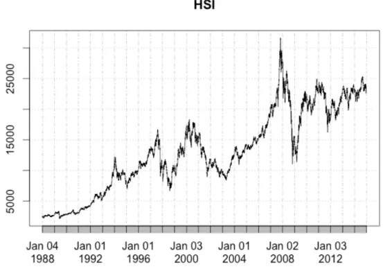
The Hang Seng Index (HSI) is a free-float capitalization-weighted index and is the most widely quoted gauge for the Stock Exchange of Hong Kong composing of the 50 largest and most liquid stocks. The index was established with a base level of 100 as of the 31st_{of July 1964, however it was not launched until the 24}th_{of November}

1969. The HSI consists of companies from various types of industries, but the financial sector occupies almost half of the industry weights in the index (47,31%). In order to better reflect the price movements of the main sectors of the market, the

(13)

index constituents stocks that are grouped into four sub-indices, namely: Finance, Utilities, Properties & Commerce and Industry. The top 5 companies listed on the HSI are HSBC Holdings, Tencent3_{, China Mobile, China Construction Bank and AIA, of}

which three of these belong to the financial sector.

Figure 3: HSI index 1988-2014.

3.2 Descriptive statistics

Our historical data has been collected from the Yahoo Finance website and covers the daily period from January 4th_{1988 until December 31}st_{2014 (over 6800}

observations). We forecast volatility for different out of sample time horizons using ARCH/GARCH models, but for now our descriptive statistics help us to begin to describe the historical data using the realized daily returns and monthly volatility. We have firstly computed the daily returns by means of the adjusted close prices of the three indices and we then go on to describe the data using statistics and graphs. We continue by calculating and analyzing the realized monthly volatility.

(14)

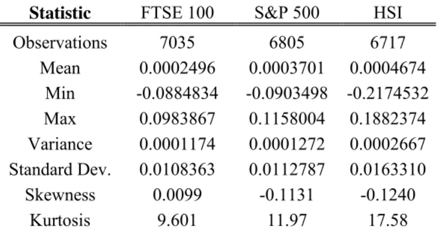
Statistic FTSE 100 S&P 500 HSI Observations 7035 6805 6717 Mean 0.0002496 0.0003701 0.0004674 Min -0.0884834 -0.0903498 -0.2174532 Max 0.0983867 0.1158004 0.1882374 Variance 0.0001174 0.0001272 0.0002667 Standard Dev. 0.0108363 0.0112787 0.0163310 Skewness 0.0099 -0.1131 -0.1240 Kurtosis 9.601 11.97 17.58

Table 1: Summary statistics of returns (FTSE, S&P500, HSI).

Since we are using three different indices, from three different countries, the number of daily observations varies due to a diverse number of trading days. We see that during the period under observation there is a larger amount of trading days in the UK and fewest in the HSI data. We estimated the returns using the following equation:

𝐫_𝐭= 𝐩𝐭− 𝐩𝐭 𝟏

𝐩_{𝐭 𝟏} (1)

Assuming that (𝑦1, 𝑦2, … , 𝑦𝑇) is a random sample of 𝑌 and 𝑇 denotes the number of observations, we can then calculate the mean as:

𝝁_𝒚= 𝟏 𝑻 𝒚𝒕

𝑻

𝒕 𝟏

(2) The mean daily return for the HSI (0.047%) is twice as large as that of the FTSE 100 (0.025%). We observe the biggest range for the Hang Seng index, which extends from -0.2175 to 0.1882 and the smallest for FTSE 100 index (from -0.0885 to 0.0984). The

standard deviations for the “western” indices are quite similar, 0.0108 and 0.0113, respectively. In the case of the HSI, the standard deviation is clearly larger (0.0163). We are specifically interested in the skewness and kurtosis since it is a measure of the shape of data distribution. Skewness measures the symmetry of a distribution and when the coefficient of skewness equals 0 (no skewness), we can say that the distribution is symmetric. If skewness < 0, the median is often greater than the mean

(15)

and the distribution is negatively skewed (distribution skewed left). The opposite holds when the skewness > 0 (distribution skewed to the right). Kurtosis, on the other hand measures the peakedness of a distribution, meaning how extreme the observations in a given data set are. The kurtosis coefficient of a normal distribution is equal to 3 (Black (2009)). We distinguish between three types, namely leptokurtic (high and thin), platykurtic (flat and spread) and mesokurtic (the most "normal" shape). By means of the same assumptions, which were used while calculating the mean return, we compute the skewness as:

𝑺(𝒚) = 𝟏 (𝑻 − 𝟏)𝝈_𝒚𝟑 (𝒚𝒕− 𝝁𝒚) 𝟑 𝑻 𝒕 𝟏 (3) and the kurtosis as:

𝑲(𝒚) = 𝟏 (𝑻 − 𝟏)𝝈𝒚𝟒 𝒚𝒕− 𝝁𝒚 𝟒 𝑻 𝒕 𝟏 (4)

From the marginally negative skewness of the S&P 500 and HSI and close to zero for FTSE 100, along with large kurtosis (>3) for all, we can deduce that the data is all similarly distributed, which is to be expected since we are only examining indices. The obtained values for skewness and kurtosis indicate that the data of returns may display the leptokurtic property (high and thin) and we approach this issue by analyzing the distribution further in the next section.

3.3 Distribution

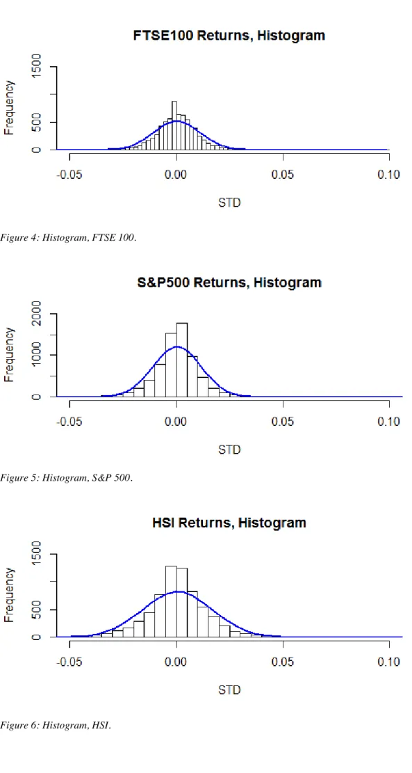
Since the distribution is of special interest in this thesis we investigate this issue through various means. Firstly, we study the histograms.

(16)

Figure 4: Histogram, FTSE 100.

Figure 5: Histogram, S&P 500.

(17)

We see in Figures 4, 5 and 6 that the leptokurtic property exists since compared to a normal distribution (Blue line), its central peak is higher and sharper, and its tails are longer and fatter. This observation is in line with the high values of kurtosis, which we obtained for each index in the previous subsection. This is consistent also with findings which states that “researchers have long noticed that stock returns have

heavy tailed probability distributions” and this is “common with financial markets data” (Ruppert (2011)). We use also the Jarque-Bera (JB) test of normality to investigate the distribution of the data. This test incorporates the squared value of the Skewness (𝑆) as well as the Kurtosis (𝐾) when it differs from its normal distribution value of 3, and is appropriate to use when there is a large number of data observations (𝑛): 𝑱𝑩 =𝒏 𝟔 𝑺 𝟐₊𝟏 𝟒(𝑲 − 𝟑) 𝟐 (5) The JB is tests the null hypothesis, which states that the data is normally distributed. The closer the Jarque-Bera statistic is to 0, the better the assumption regarding normality of distribution (Gujarati (2014)).

Jarque-Bera Normality Test

FTSE100 S&P500 HSI

Statistic 12771.3206 22834.2915 59522.4236

p-value 2.2e-16 2.2e-16 2.2e-16

Table 2: Jarque-Bera test statistics. If the p-values are smaller than the critical value (5%), we can reject the null hypothesis, which states that the examined indices are normally distributed. Else, fail to reject.

Such small p-values (<0.05) related to the JB statistic suggests that we can reject the null hypothesis, meaning, the data is not normally distributed. We have also included the quantile plots (Figure 7). The points should fall approximately on a straight line if the data is normally distributed. We do not observe such a pattern in any of the plots

presented below. This kind of point’s location, obtained for all three indices, suggests that the data is heavily tailed compared to that of the normal distribution.

(18)

Figure 7: Normal Q-Q Plots for FTSE 100, S&P 500 and HSI, respectively. In the case where the data follows the assumed (normal) distribution, the points should fall approximately on a straight line.

(19)

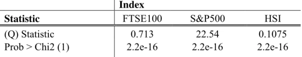
3.4 Ljung-Box Q-Test

The autocorrelation function is applied to collect information about the properties of a time series (Koop (2006)). The best way to test for quantification of the autocorrelation is using the Ljung-Box Q-Test, which is able to check whether the data is random and independent. In the case where the observations are not independent, we can see a correlation between adjacent observations (autocorrelation). The Ljung-Box Q-test examines the null hypothesis, which states that the data is independently distributed up to lag ℓ𝓁 (no autocorrelation), versus the alternative hypothesis where the data is not random and independent (autocorrelation is present). The Ljung-Box test statistic is as follow:

𝓠(𝒎) = 𝑻(𝑻 + 𝟐) 𝝆𝓵 𝟐 𝑻 − 𝓵 𝒎 𝓵 𝟏 (6) Where,

𝜌_ℓ𝓁- estimated autocorrelation of the series at lag ℓ𝓁, 𝓂 - denotes degrees of freedom (the largest lag), 𝑇 - observed data point.

Index

Statistic FTSE100 S&P500 HSI

(Q) Statistic 0.713 22.54 0.1075

Prob > Chi2 (1) 2.2e-16 2.2e-16 2.2e-16

Table 3: Ljung-Box test. If the Q–value is larger than the critical value (5%), we can reject the null hypothesis that states that there is noautocorrelation in the returns. Else, fail to reject.

We can reject the null hypothesis when 𝑄 is larger than χ (the chi-square distribution value with ℎ degrees of freedom and significance level 𝛼). Therefore, all three indices exhibit autocorrelation (Box (1978)).

(20)

3.5 Volatility

We forecast volatility for 1, 3, 6, 9 and 12 months thus, for the sake of simplicity, we adjust the computed daily returns by assuming that there are 21 trading days in a month.

In order to calculate the realized (actual) volatility for month 𝑖, we select the returns for a given month 𝑟, where 𝑡 = {1, 2, … , 𝑁}, and 𝑁 represents the number of days in a month. To calculate the daily-realized volatility, we use the following formula, which squares the difference between the return and the mean return before dividing it by the number of observation minus one and then applying the square-root function:

𝝈_𝒊𝒅𝒂𝒊𝒍𝒚 = ∑ (𝒓𝒕− 𝚬[𝒓𝒊]) 𝟐 𝑻 𝒕 𝟏 𝑵 − 𝟏 (7) Where:

𝐸[𝑟 ] - mean daily return for 𝑖 month, 𝜎 - realized volatility for 𝑖 month.

In practice it is more common to use a simpler formula to calculate the realized volatility: 𝝈_𝒊𝒅𝒂𝒊𝒍𝒚= ∑ 𝒓𝒕 𝟐 𝑻 𝒕 𝟏 𝑵 (8) The main reason for this is that 𝐸[𝑟 ] is virtually zero. Moreover, the difference between dividing by 𝑁 and 𝑁 − 1 is insignificant when working with a large number of observations.

Both formulas presented above give us the daily volatility. In order to adjust it to our needs for forecasting horizons we re-compute equation (8) to the monthly volatility by means of the square root rule and based on our assumption of trading days outlined

(21)

above. Moreover, we computed the summary statistics of realized monthly volatility of all three indices.

Index Min

1st

Quantile Median Mean

3rd

Quantile Max

FTSE 100 5.63 10.20 12.70 15.20 17.90 75.90

S&P 500 4.91 10.20 12.90 15.50 18.20 82.10

Hang Seng 6.99 14.30 18.60 22.30 26.40 110.00

Table 4: Realized monthly volatility statistics.

We observe that the volatility statistics for the FTSE 100 and S&P 500 are very similar, whereas the HSI is similar only in the minimums. A larger difference can be seen in the mean. It takes a value of around 15% for the FTSE 100 and S&P 500, while the mean of the HSI is around 42% larger (22%). Another noticeable difference can be seen in the maximums where the HSI is extreme compared to that of the FTSE 100 and S&P 500.

Regressing the volatility on the lagged volatility for one period results in a 𝑅 = 0.4993, 0.5220 and 0.2530 for the three indices respectively. This indicates that the variation in volatility is not greatly explained by the previous period’s volatility for the HSI index whereas for the FTSE and S&P the variation is around 50%. For all of the indices we increase the lag by one period at a time untill the last periods coeffiecient are no longer statistically significant (p>0.05). It become not significant for the variable lagged twice for the FTSE, three times for the S&P 500 and four time for the HSI index.

Figures 8, 9 and 10, present the realized monthly historical volatility for the three indices. There are no obvious common patterns that can be observed. Yet, there are some similarities in the volatility of the FTSE and the S&P indices, which are almost identical over the whole period (this is in line with the summary statistics from Table 4. For these two indices, the most sudden changes are observed at the turn of 2000-2002 (dot-com bubble crash) and during the most recent financial crises (2007/2008). The HSI peaks in 1987, 1997 and 2007/2008 and are all caused by financial crises. An interesting observation is that the most recent financial crisis seems to have resulted in

(22)

two after effects for the FTSE and S&P where as the volatility of the HSI has only dramatically increased once since.

Figure 8: Realized monthly historical volatility of the FTSE 100 index.

Figure 9: Realized monthly historical volatility of the S&P 500 index.

(23)

4. Methodology

The methodology section presents the naïve model and the forecasting model that is used by the ARCH/GARCH family models along with the individually described error distributions before presenting the forecasting evaluation and predictive power statistics. The ARCH/GARCH models are used in the forecasting of volatility and we have introduced the model with the largest number of restrictions first. We have then expanded our model selection with the motivation of including models that remove some restrictions and limitations with the hope of achieving an insight into whether the more complicated models offer better forecasting predictions over our selected horizons.

4.1 Naive Forecasting Model

This straightforward and simple model forecasts based on the previous known observations. It treats the last period’s volatility as this period’s volatility (Giusti, Ritter and Vichi (2012)).

𝜎 = 𝜎 (9)

The biggest weakness of this model is that the volatility is too persistent and does not perform well with long-run predictions (Zakamulin (2014)). We include the naive model as a benchmark for which to measure the more technical models against.

4.2 Rolling window

A rolling window forecast generates a series of forecasted observations for a given number of steps ahead. By using this method we define a fixed length of the in-sample period and a specific step size, meaning that the first and last date increase by the assigned value of observations/steps at each time. We use a 5-year rolling window and for simplicity assume that there is 21 trading days in a month (regardless of the country), which gives us 1260 observations. There are over 6800 daily observations for each index, so for example the first rolling window of the FTSE 100 contains data from day 1 to 1260. Then, by means of the model we obtain the forecast for the next day (observation number 1261) and thus, the second sample covers the observations from day 2 until day 1261. Based on the second sample we forecast observation

(24)

contain observations from 5775 to 7035. We repeat this operation for all three indices whilst varying the step size based on the desired forecasting horizon.

4.3 ARCH

The Autoregressive Conditional Hetroskedasticity (ARCH) model was developed by Engle (1982). The main idea behind this model is that the mean corrected asset return is serially uncorrelated and dependent, meaning that ARCH is based on a linear regression where the variable, in time series form, varies around the mean (𝜇) randomly. Moreover, the model can be defined by the quadratic function of its lagged values. We assume that the return on assets can be computed as:

𝑟 = 𝜇 + 𝜎 𝜖 (10)

Where 𝜖 is a sequence of 𝑁(0,1) independent and identically distributed (i.i.d.) random variables. We can then describe the residual return (𝑟 − 𝜇) at time 𝑡, as:

𝑍𝑡 = 𝜎 𝜖 (11)

Therefore, the ARCH model, which presents conditional variance as 𝜎 , can be expressed as follows:

𝜎 = 𝛼 + 𝛼 𝑍

(12) Where 𝛼 > 0 and 𝛼 ≥ 0.

The lag length (𝑡 − 𝑘) of the ARCH model to the in-sample data is chosen in this thesis by the AIC, SBIC, HQIC in section 5. Lower order ARCH models may not be the most accurate in forecasting volatility due to the number of restrictions. We still include the ARCH model as it provides the basis of the parameters for the GARCH models that we wish to study further due to their handling of the previously stated issues. The main weakness is that the squared shocks model the conditional variance, and this leads to the ARCH model not being able to distinguish between positive and

(25)

negative effects, otherwise known as asymmetric effects. Another drawback is that recent evidence suggests that there exists substantial persistence in the variance of such models (Lamoureux and Lastrapes (1990)). The ARCH model also carries mean reverting properties which suggests that the process reverts to its mean slowly therefore remaining highly persistent for long periods before returning to the equilibrium, but due to its restrictive intervals it causes the volatility to often be over predicted owing to a slow response to shocks.

The ARCH model´s strengths lie in the fact that it can model volatility clustering through the lagged squared returns of 𝑍 which is described as “large changes tend

to be followed by large changes, of either sign, and small changes tend to be followed

by small changes” (Mandelbrot (1997)).

4.4 GARCH

Bollerslev (1987) developed the Generalized Autoregressive Conditional

Hetroskedasticity (GARCH) model, which is an extension of the ARCH model where the order of ARCH (𝑡) (𝛼 𝑍 ), as established previously, is built upon to include the GARCH term 𝛽 𝜎 . The model is as follows:

𝝈_𝒕𝟐= 𝜶_𝟎+ 𝜶_𝒌 𝒑 𝒌 𝟏 𝒁_{𝒕 𝒌}𝟐 + 𝜷_𝒋 𝒒 𝒋 𝟏 𝝈_{𝒕 𝒋}𝟐 (13)

The GARCH model is said to be “much more flexible and capable of matching a wide variety of patterns of financial volatility” (Koop (2006)). The GARCH again deals with volatility clustering and is characterized by a symmetric response of current volatility to positive and negative returns. It also has the addition of 𝜎 , the lagged conditional variance, which helps to increase the accuracy of the ARCH model by avoiding excessive lags of the squared returns. Both ARCH’s and GARCH’s biggest

weakness lies in the fact that the models assume that the shocks (both positive and negative) have the same effects on volatility which is generally accepted not to be

(26)

Unlike the conditional variance, which is changing, the unconditional variance of 𝑍 is constant if the assumption of mean reversion is maintained (𝛼 + 𝛽 < 1) and can be expressed as:

𝜎 = 𝛼

1 − 𝛼 − 𝛽 (14)

Otherwise, when 𝛼 + 𝛽 ≥ 1, we say that the unconditional variance of 𝑍 is not defined, meaning we face a “non-stationarity” in variance. Moreover, in the case where 𝛼 + 𝛽 = 1, we have a “unit root” in variance (Brooks (2014)).

4.5 EGARCH

In order to deal with the weaknesses of the GARCH model, which assumes that positive and negative shocks affect volatility equally, we use the Exponential GARCH (EGARCH), which was introduced and modeled by Nelson (1991). This is an asymmetric form of the GARCH model. The EGARCH is able to respond asymmetrically to positive and negative effects as well as the volatility persistence and mean reversion. The model is formally written as, an EGARCH (𝑝, 𝑞):

𝑙𝑜𝑔(𝜎 ) = 𝛼 + [𝛼 𝑍 + 𝛾 |𝑍 | − 𝐸(|𝑍 |) ] + 𝛽 log(𝜎 )

(15) The section in the squared brackets illustrates the models ability to deal with the asymmetric effects of positive and negative returns. The function has a mean of zero and is uncorrelated. It can be re-written as:

(𝜶𝟏+ 𝜸𝟏)𝒁𝒕𝑰(𝒁𝒕> 𝟎) + (𝜶𝟏− 𝜸𝟏)𝒁𝒕𝑰(𝒁𝒕< 𝟎) − 𝜸𝟏𝑬(|𝒁𝒕 𝟏|) (16)

Where (𝛼 + 𝛾 ) takes the positive shocks into consideration and (𝛼 − 𝛾 ) deals with the negative shocks. This gives rise to the leverage effect which states that negative shocks have a larger impact than positive shocks since 𝛼 < 0, 0 ≤ 𝛾 ≥ 0 𝑎𝑛𝑑 𝛽 + 𝛾 < 1. The shocks impact the logarithm of the conditional variance

(27)

𝑙𝑜𝑔(𝜎 ). Since log (𝜎 ) is the log of the variance, the conditional variance is guaranteed to be positive, therefore not artificially imposing non-negativity on the model parameters and the model allows for asymmetries (Brooks (2014)). A possible drawback of the EGARCH model is that it does not fit the normal distribution and under normality it tends to overestimate the impact of outliers. This is an interesting aspect and the findings between the normal, student-t and generalized error distributions will be of special interest for this model.

4.6 GJR-GARCH

We use the GJR-GARCH as another asymmetric model since we would still like to take into consideration the different impacts that positive and negative innovations have and since the EGARCH model is highly dependent on the data not being normally distributed we will closely compare these two models.

The model was presented by Glosten, Jagannathan and Runkle (1993) and the difference between the EGARCH and the GJR-GARCH model is a slight change in the conditional variance function which is no longer a logarithm and the positive and negative shocks are seen through 𝛾 and 𝛼 respectively.

𝝈_𝒕𝟐= 𝜶𝟎+ [𝜶𝒌𝒁𝟐𝒕 𝒌(𝟏 − 𝑰[𝒁𝒕 𝒌> 𝟎]) + 𝜸𝒌𝒁𝒕 𝒌𝟐 𝑰[𝒁𝒕 𝒌 > 𝟎]) 𝒑 𝒌 𝟏 + 𝜷𝒋 𝒒 𝒋 𝟏 𝐥𝐨𝐠(𝝈_{𝒕 𝒋}𝟐 ) (17)

4.7 Distribution statistics

Normal distribution (Gaussian)

The Normal or Gaussian distribution is an absolute continuous distribution where the mean is equal to zero and the variance is equal to one (𝑁 (0,1)). For the normal distribution we observe zero skewness and zero excess kurtosis. It is the most

(28)

commonly used distribution within financial analysis since it is symmetric and requires only the mean and variance.

𝒇(𝒙, 𝝁, 𝝈) = 𝟏 𝝈√𝟐𝝅𝒆 (𝒙 𝝁)𝟐 𝟐𝝈𝟐 (18) Student t-distribution

As we have seen in (Section 3.3) our in-sample data does not fit a standard normal distribution. We therefore consider the student t-distribution, first derived by Helmert (1876) but formally written by Gosset (1908) under the pseudonym “Student”. This

distribution can work with smaller sample sizes, which are considered through 𝑣 = 𝑛 − 1 degrees of freedom. 𝒇(𝒕) = 𝚪 𝒗 + 𝟏 𝟐 √𝒗𝝅𝚪 𝒗_𝟐 (𝟏 +𝒕 𝟐 𝒗) 𝒗 𝟏 𝟐 (19) The student t-distribution has, similarly to the normal distribution, zero skewness (it is symmetric) but excess kurtosis equal to for 𝑣 > 4 (leptokurtic property).

Generalized error distribution

The generalized error distribution (GED) was introduced by Subbotin (1923) (Agro (1995)). This distribution is used when the errors of the data are not necessarily normally distributed. Vasudeva and Kumari (2013), discuss the first class of GED (GED-I) from the parametric family of symmetric distributions, which we have used, since it can cope with the heavier tailed symmetric distributions of our data and can become a useful way to parameterize (Nadarajah (2005)).

𝒅𝑭(𝒙|𝝁, 𝝈, 𝜿) = 𝒆 𝟏 𝟐 𝒙 𝝁 𝝈 𝟏 𝒌 𝟐𝒌 𝟏_{𝝈𝚪(𝒌 + 𝟏)}𝒅𝒙 (20)

(29)

Where 𝑥 is the domain of the p.d.f and the distribution is defined by 𝜇, 𝜎, 𝑘, which relates to the mode, dispersion and skewness of the data respectively. The generalized error distribution has symmetric properties but allows for variation in the kurtosis which are considered to be close to the normal distribution (Giller (2005)).

4.8 Forecast Evaluation

There exist various methods that allow us to compare how well the models can predict the dependent variable. We use the mean squared error (MSE) to analyze the quality of the ARCH and GARCH family models so that our findings can be directly compare to existing research.

The MSE is often used in comparing the difference between things that vary from an accepted standard. It is highly dependent on the scale of the dependent variable with the smaller the MSE of the model suggesting the better the models ability. We first predict the volatility, and then compute the realized volatility, at the end we compare our results by means of the following formula:

𝑴𝑺𝑬 = 𝟏 𝒏 (𝝈𝒊− 𝝈𝒊) 𝟐 𝒏 𝒊 𝟏 (21) 𝑴𝑺𝑬 = 𝟏 𝒏 𝒆𝒊 𝟐 𝒏 𝒊 𝟏 (22) Where:

𝜎 - actual value of the 𝑖 observation, 𝜎 - forecasted value of the 𝑖 observation, 𝑒 - forecasting error of the 𝑖 observation, 𝑛 - number of observations.

The main weakness of this method is that the prediction error variance varies across time. This problem is also common among other similar measurement techniques

(30)

approaches zero (0 means that there is no difference between what was predicted and what actually happened). We compare the findings for each index over the three chosen distribution statistics.

4.9 Predictive Power

Together with a method that helps us to evaluate the goodness of forecast, we will also compute the predictive power of each model over the different forecasted time horizons. To do this, we use a method proposed by Blair, Poon and Taylor (2010). The predictive power is a comparison between the prediction errors and the variation in 𝜎 , which are both squared. The closer the predictive power ratio is to one hundred the better the accuracy of the forecasted volatility. Any deviation suggests that there exists greater variation of the errors of the forecasted volatility than those of the realized volatility. The predictive power (𝑃) can be both positive and negative (Poon (2005)): 𝑷 = 𝟏 −∑𝒏𝒊 𝟏(𝝈𝒊 𝝈𝒊)𝟐 ∑𝒏𝒊 𝟏(𝝈𝒊 𝝈)𝟐 × 𝟏𝟎𝟎 (23) Where:

𝑛 - number of out-of-sample observations, 𝜎 - realized volatility,

𝜎 - forecasted volatility, 𝜎 - mean value of volatility.

The mean value of volatility in the out-of-sample period can be computed as:

𝝈 =𝟏 𝒏 𝝈𝒊

𝒏 𝒊=𝟏

(31)

5. Results

We first provide an initial look at the of lag length selection through observation of the auto and partial-auto correlation functions based on the daily returns where we distinguish a rough estimation of the ARMA (p,q). We then acquire the (p,q) more

accurately using the Akaike's information criterion (AIC), Schwarz’s Bayesian information criterion (BIC), and the Hannan and Quinn information criterion (HQIC). We then look at the significance of the parameters of GARCH, E-GARCH and GJR-GARCH (1,1) models and look each of the parameters individually. For the higher order models ((1,2) (2,1) (2,2)) we compare AIC statistics. We present the MSE and predictive power values for 1, 3 6, 9 and 12 months forecasting periods. We also compare the models on the time horizon with the best forecast evaluation with the higher order models selected from the lowest AIC statistic, in order to gain an insight into the advantages or disadvantages of using higher order models.

(32)

5.1 FTSE100

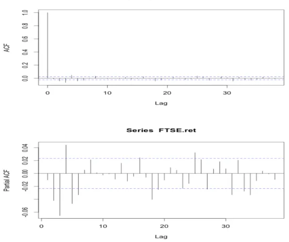
Figure 11: Auto and Partial-Auto correlation functions for the FTSE 100 index.

The ACF and PACF exhibit significant autocorrelations in the residuals and both have their first significant autocorrelation visible already at lag 2. The ACF is significant at lags 6 and 8, after which it gradually fades away. The PACF is significant in lags 2-6 and also has the tendency of fading away. This would suggest that an ARMA (p,q) is present and a higher order model could be necessary. These results are also confirmed in the test statistics of lag length selection models presented below.

(33)

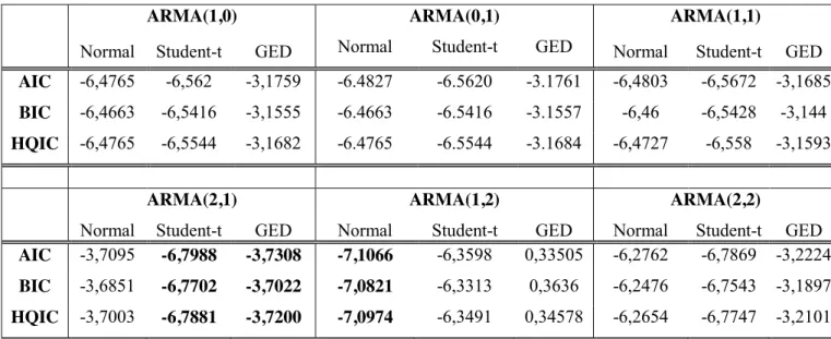
Table 5: FTSE 100 Information Criteria for model selection of the Auto Regressive Moving Average (ARMA).

The specifications for the conditional variance, given in Table 5, contain parameters for the auto regressive and moving average, denoted by 𝑝 and 𝑞. We have included six combinations of ARMA lengths. For the normally distributed model, 𝑝 and 𝑞 are the lowest at ARMA (1,2) and for the t-distribution ARMA (2,1). The GED also shows an improvement when, 𝑝 and 𝑞 ARMA order is (2,1). The AIC, BIC and HQIC for the normal distribution become positive at (3,2), (2,3) and (3,3) and increase for the other two distributions. In order for our ARCH/GARCH models to remain reasonable and comparable and to forecast the same models on each index we keep the ARMA length at (1,1). Since models with large amounts of lags rarely give more accurate results than the same models with fewer lags, it is rational to assume, that this small modification regarding ARMA (p,q) will not result in any disturbance in our analysis. Using the lag length of (1,1) also keeps our research in-line and comparable with the work which were summarized in the literature review section of this thesis (Section 2).

Using ARMA (1,1) we compare the GARCH, EGARCH and GJR-GARCH models under the three error distributions and select the optimal order of models beginning at (1,1), whilst also extending them to higher order models if necessary.

ARMA(1,0) ARMA(0,1) ARMA(1,1)

Normal Student-t GED Normal Student-t GED Normal Student-t GED

AIC -6,4765 -6,562 -3,1759 -6.4827 -6.5620 -3.1761 -6,4803 -6,5672 -3,1685

BIC -6,4663 -6,5416 -3,1555 -6.4663 -6.5416 -3.1557 -6,46 -6,5428 -3,144 HQIC -6,4765 -6,5544 -3,1682 -6.4765 -6.5544 -3.1684 -6,4727 -6,558 -3,1593

ARMA(2,1) ARMA(1,2) ARMA(2,2)

AIC -3,7095 -6,7988 -3,7308 -7,1066 -6,3598 0,33505 -6,2762 -6,7869 -3,2224 BIC -3,6851 -6,7702 -3,7022 -7,0821 -6,3313 0,3636 -6,2476 -6,7543 -3,1897

(34)

FTSE

100 GARCH(1,1) EGARCH(1,1) GJR-GARCH(1,1)

mu 0,00048 0,000251 0,000456 0,000068 -0,000053 0,000187 0,00013 -0,000073 0,000219 s.e 0,000226 0,000152 0,00021 0,000084 0,000171 0,000194 0,000216 0,000197 0,000169 p-value 0,033449 0,097789 0,029637 0,41487 0,757603 0,33579 0,54601 0,711519 0,19472 omega 0,000002 0,000001 0,000002 -0,36703 -0,119368 -0,37034 0,000003 0,000001 0,000003 s.e 0,000002 0,000004 0,000003 0,007283 0,003255 0,00569 0 0,000002 0 p-value 0,354979 0,778516 0,529729 0 0 0 0 0,361531 0 alpha1 0,096327 0,10161 0,096325 -0,14235 -0,120732 -0,15779 0 0 0 s.e 0,030046 0,063243 0,043353 0,009031 0,003255 0,016323 0,004826 0,021445 0,006231 p-value 0,001346 0,108127 0,026291 0 0 0 1 0,999995 0,99998 beta1 0,879383 0,892257 0,883401 0,960921 0,987434 0,961371 0,876258 0,913898 0,871061 s.e 0,036675 0,061892 0,051184 0,000763 0,000028 0,000123 0,014238 0,024565 0,017622 p-value 0 0 0 0 0 0 0 0 0 shape 12,93365 1,322303 21,069995 1,397429 18,675424 1,409927 s.e 1,199575 0,054445 8,820335 0,070228 8,858992 0,082652 p-value 0 0 0,016904 0 0,035024 0 ar1 -0,94889 0,868502 -0,96733 -0,94844 0,530585 -0,96139 -0,95245 0,612553 -0,96724 s.e 0,010101 0,138921 0,006196 0,003954 0,044616 0,002677 0,008485 0,224405 0,005997 p-value 0 0 0 0 0 0 0 0,00634 0 gamma1 0,145409 0,075922 0,149203 0,186358 0,142047 0,201142 s.e 0,043415 0,012064 0,015416 0,027435 0,030648 0,032638 p-value 0,00081 0 0 0 0,000004 0 ma1 0,9684 -0,91144 0,984307 0,967237 -0,5849 0,978779 0,971924 -0,680342 0,984318 s.e 0,003588 0,118393 0,000643 0,00465 0,042505 0,000715 0,002585 0,208171 0,000639 p-value 0 0 0 0 0 0 0 0,001082 0 FTSE

AIC -6,6383 -6,4165 -6,6736 -6,6848 -6,4539 -6,7115 -6,6896 -6,4347 -6,7139

BIC -6,6138 -6,3879 -6,6450 -6,6562 -6,4212 -6,6788 -6,6611 -6,4020 -6,6813 HQIC -6,6291 -6,4057 -6,6629 -6,6741 -6,4416 6,6992 -6,6789 -6,4224 -6,7016

Table 6: GARCH (1,1) family models statistics and information criteria for the FTSE100 index. The values which are not statistically different from zero are highlighted in blue.

Our results show that based on the assumption of 5% significance the parameters of the GARCH models are all significantly different from zero apart from omega for all

(35)

distributions and mu and omega for the student t-distribution. The EGARCH is not significant in its mean for all three distributions. The GJR parameters are not significance in the mean and alpha. These findings suggest that higher order model would maybe be more appropriate. We have therefore looked at the AIC of the higher order models and our findings suggest that the GARCH (2,2), EGARCH (2,1) and GJR-GARCH (1,1) should be used, however to keep our results comparable to previous research and due to the minor differences in the AIC statistic we have chosen to forecast all of our models as (1,1). We do however present the results for the higher models over a 1 month forecasting horizon in order to prove that the higher order models selected based on the lower AIC statistic do not significantly enhance the results.

FTSE

100 GARCH EGARCH GJR-GARCH

AIC(1,1) -6,6383 -6,6603 -6,6736 -6,6848 -6,7059 -6,7115 -6,6896 -6,7061 -6,7139 AIC(2,1) -6,6383 -6,6613 -6,6738 -6,6876 -6,7081 -6,7126 -6,6866 -6,703 -6,7107 AIC(1,2) -6,6367 -6,6587 -6,6720 -6,6832 -6,7042 -6,7098 -6,6881 -6,7045 -6,7123 AIC(2,2) -6,6387 -6,6623 -6,6741 -6,6860 -6,7066 -6,7111 -6,6850 -6,7014 -6,7091

Table 7: Akaike´s Information Criteria of higher order GARCH family models for the FTSE 100 index.

In Table 8 and Figure 12 below we present our findings and observe that the MSE gives the best results for a 1 month forecast. The 1 month forecast is better than the longer forecasted horizons and all of the ARCH/GARCH models give more accurate results when using the student t-distribution whereas the naïve model performs best with the normal and generalized distribution. For the 1 month forecast the benchmark naïve model is outperformed by all other models.

(36)

Table 8: MSE forecasting results for the FTSE 100 index over multiple time horizons.

Figure 12: Clustered Column Chart of FTSE 100 MSE results.

0 0.02 0.04 0.06 0.08 0.1 0.12 0.14 0.16 Norm al St ud ent t GED Norm al St ud ent t GED Norm al St ud ent t GED Norm al St ud ent t GED Norm al St ud ent t GED 21 63 126 189 252 MSE

FTSE 100

Naive ARCH GARCH(1,1) EGARCH(1,1) GJR-GARCH(1,1)

MSE

nDays Distribution Naive ARCH GARCH(1,1) EGARCH(1,1) GJR-GARCH(1,1)

21 Normal 0,000355 0,012210 0,0003214 0,0002826 0,0002741 Student t 0,001148 0,000289 0,0001309 0,0001091 0,0001144 GED 0,000355 0,002392 0,0003198 0,0002844 0,0002734 63 Normal 0,001148 0,028010 0,0009224 0,0008503 0,0007975 Student t 0,000473 0,000851 0,0004323 0,0003219 0,0003373 GED 0,001148 0,007381 0,0009239 0,0008789 0,0008092 126 Normal 0,002759 0,03401 0,002148 0,001808 0,001677 Student t 0,001260 0,00195 0,000935 0,000801 0,000690 GED 0,002759 0,01497 0,002097 0,001887 0,001694 189 Normal 0,003526 0,13810 0,002975 0,002754 0,002453 Student t 0,003526 0,02750 0,002836 0,002862 0,002501 GED 0,003526 0,02257 0,002837 0,002871 0,002511 252 Normal 0,006815 0,08425 0,008209 0,005658 0,005823 Student t 0,006815 0,02884 0,007566 0,005617 0,005725 GED 0,006815 0,03060 0,007848 0,005746 0,005820

(37)

The most accurate forecasting horizon for the predictive power is 1 month where all student t-distribution models outperform that of the normal and generalized distribution. The naïve model outdoes ARCH (1,1) and is only slightly worse than GARCH (1,1). The most accurate results are given by the EGARCH (1,1) model. Although the Predictive power does decrease as the time horizon increases, this is seen to only be marginal in the case of the models with the student t-distribution , up to and including the 6 month (126 day) forecasting horizon. These results seem to be disproportionally high and have been retested multiple times to check there accuracy.

Predictive Power

nDays Distribution Naive ARCH GARCH(1,1) EGARCH(1,1) GJR-GARCH(1,1)

21 Normal 44,4 -1811 49,68 55,75 57,09 Student t 80,09 59,47 81,64 84,69 83,95 GED 44,4 -274,5 49,93 55,48 57,19 63 Normal 28,55 -1643 42,61 47,09 50,38 Student t 77,12 58,81 79,07 84,41 83,67 GED 28,55 -359,2 42,52 45,31 49,65 126 Normal 3,021 -1095 24,49 36,46 41,06 Student t 69,08 52,12 77,06 80,35 83,07 GED 3,021 -426,2 26,29 33,67 40,47 189 Normal 6,044 -3580 20,73 26,62 34,64 Student t 6,044 -632,7 24,44 23,73 33,35 GED 6,044 -501,3 24,42 23,51 33,1 252 Normal -33,1 -1545 -60,33 -10,50 -13,74 Student t -33,1 -463,3 -47,77 -9,701 -11,82 GED -33,1 -497,6 -53,27 -12,22 -13,66

Table 9: Predictive Power forecasting results for the FTSE 100 index over multiple time horizons.

When comparing the results against the higher order models selected based on the lowest AIC, we observe no improvement in the models MSE or predictive power where there was only a slight loss for GARCH (2,2).

(38)

MSE

21 Normal 0,0003552 0,009101 0,0003214 0,0002817* 0,0002741

Student t 0,0001418 0,0002888 0,0001315 0,0001091 0,0001144

GED 0,0003552 0,002392 0,0003174* 0,0002833* 0,0002734

Predictive Power

21 Normal 44,4 -1325 49,75* 55,9* 57,1

Student t 80,09 59,47 81,55 84,69 83,95

GED 44,4 -274,5 50,31* 55,65* 57,19

Table 10: MSE and Predictive Power forecasting results for higher order GARCH AND EGARCH models over a 21 day forecasting horizon. Values marked with an asterisk (*) show an improvement.

(39)

5.2 S&P 500

Figure 13: Auto and Partial-Auto correlation functions for the S&P 500 index.

The ACF cuts off after the second lag. This behavior indicates an MA (2) process. The PACF also cuts off after the second lag, indicating an AR (2) process but the correlogram shows the larger correlation in higher lags such as 5, 7, 10 and 12. All three information criteria statistics suggest that in the case of the normal and student t-distributions that ARMA (1,1) produces the lowest statistics. For the generalized distributions the best is ARMA (2,1). The values obtained in ARMA (2,2) for the normal and student t-distributions vary significantly and become positive or are not obtainable in R. We therefore select to continue our analysis with the ARMA (1,1) model.

(40)

ARMA(1,0) ARMA(0,1) ARMA(1,1)

AIC -6.3978 -6.5661 -2.6646 -6.3977 -6.5660 -2.6612 -6.4039 -6.5715 -2.7159 BIC -6.3815 -6.5457 -2.6442 -6.3814 -6.5456 -2.6408 -6.3835 -6.5470 -2.6914 HQIC -6.3917 -6.5584 -2.6569 -6.3916 -6.5584 -2.6535 -6.3962 -6.5623 -2.7067

ARMA(2,1) ARMA(1,2) ARMA(2,2)

AIC -6.5710 -2.7135 -2.9071 -6.5639 -2.7260 385.84 -2.7234 BIC -6.5424 -2.6850 -2.8827 -6.5353 -2.6975 385.88 -2.6908

HQIC -6.5603 -2.7028 -2.8979 -6.5532 -2.7153 385.86 -2.7111

Table 11: S&P500 Information Criteria for model selection of the Auto Regressive Moving Average (ARMA).

In Table 12 our results show that EGARCH (1,1) is significantly different from zero for all distributions and GARCH is again not significant in omega. GJR-GARCH is not statistically significant in alpha for all distributions and AR (1) and MA (1) with the normal distribution.

(41)

S&P

mu 0,000681 0,000765 0,000981 0,000312 0,000727 0,000662 0,000471 0,000682 0,000662

s.e 0,000031 0,000043 0,000122 0,000106 0,000176 0,000033 0,000201 0,000032 0,000033

p-value 0 0 0 0,003201 3,50E-05 2,00E-06 0,018936 0 0,0000E+00

omega 0,000003 0,000003 0,000003 -0,49701 -0,46257 -0,51395 0,000003 0,000004 0,000004 s.e 0,000002 0,000002 0,000002 0,005284 0,007278 0,008199 0 0 0 p-value 0,15606 0,089678 0,15793 0 0 0 0 0 0 alpha1 0,14213 0,152062 0,143579 -0,22036 -0,24961 -0,23122 0 0 0 s.e 0,020458 0,028887 0,026431 0,01651 0,024397 0,026379 0,010072 0,010431 0,009414 p-value 0 0 0,031085 0 0 0 0,999999 0,99999 1,00E+00 beta1 0,82469 0,821367 0,822839 0,947161 0,95257 0,947264 0,838845 0,800636 0,808844 s.e 0,025721 0,028626 0,031085 0,000229 0,000476 0,001038 0,01455 0,019685 0,017864 p-value 0 0 0 0 0 0 0 0 0 shape 5,548586 1,272639 5,821013 1,331867 6,111765 1,361226 s.e 0,935857 0,070512 1,004069 0,069237 1,032129 0,074012 p-value 0 0 0 0 0 0,00E+00 ar1 0,961876 0,961661 0,918547 -0,87803 0,526459 0,750844 -0,84899 0,969699 0,971911 s.e 0,00425 0,005266 0,015172 0,031641 0,057167 0,06747 1,709544 0,003455 0,003817 p-value 0 0 0 0 0 0 0,619456 0 gamma1 0,152124 0,143476 0,157328 0,244052 0,292037 0,270568 s.e 0,01125 0,015698 0,010672 0,036007 0,048059 0,043926 p-value 0 0 0 0 0 0 ma1 -0,99349 -0,99135 -0,95319 0,867427 -0,55909 -0,77742 0,838975 -0,99295 -0,992798 s.e 0,000125 0,00012 0,007955 0,03299 0,054959 0,062389 1,764539 0,000103 0,000087 p-value 0 0 0 0 0 0 0,634456 0 0 S&P

Normal Student-t GED Normal Student-t GED Normal Student-t GED AIC -6,6656 -6,7025 -6,708 -6,7112 -6,7496 -6,7515 -6,7027 -6,7469 -6,7500 BIC -6,6411 -6,6740 -6,6794 -6,6827 -6,7170 -6,7188 -6,6741 -6,7143 -6,7174 HQIC -6,6564 -6,6918 -6,6972 -6,7005 -6,7374 -6,7392 -6,6919 -6,7347 -6,7378

(42)

The AIC for the higher order models suggest an improvement could be found through higher order models. The AIC suggests (2,1) for the GARCH and EGARCH models and due to no improvement in the AIC for the GJR GARCH, (1,1) is selected despite the non-significant alpha, AR (1) and MA (1) in the normal distribution. The results are again calculated using the (1,1) on all models and directly compared with the results of the best AIC models.

S&P 500 GARCH EGARCH GJR-GARCH

AIC(1,1) -6,6656 -6,7025 -6,708 -6,7112 -6,7496 -6,7515 -6,7027 -6,7469 -6,75 AIC(2,1) -6,6756 -6,7096 -6,7153 -6,731 -6,7647 -6,7669 -6,7022 -6,7458 -6,7486 AIC(1,2) -6,6647 -6,7013 -6,7068 -6,7114 -6,7495 -6,7511 -6,7026 -6,7462 -6,7493 AIC(2,2) -6,6752 -6,5376 -6,7141 -6,7296 -6,5838 -6,7656 -6,7109 -6,5471 -6,7535

Table 13: Akaike´s Information Criteria of higher order GARCH family models for the S&P 500 index.

MSE

21 Normal 0,0004123 0,023860 0,0003609 0,0003643 0,0003248 Student t 0,0004123 0,006222 0,0003610 0,0003462 0,0003251 GED 0,0004123 0,002632 0,0003606 0,0775100 0,0003219 63 Normal 0,001524 0,04183 0,001291 0,001503 0,001250 Student t 0,001524 0,05242 0,001295 0,001437 0,001219 GED 0,001524 0,008115 0,001295 0,001502 0,001233 126 Normal 0,003708 0,03713 0,003348 0,003486 0,003251 Student t 0,003708 0,1531 0,003597 0,003453 0,003223 GED 0,003708 0,01637 0,003495 0,003586 0,003254 189 Normal 0,005624 0,07937 0,003961 0,00497 0,004226 Student t 0,005624 0,4221 0,004125 0,005161 0,0045 GED 0,005624 0,02466 0,004121 0,005483 0,004352 252 Normal 0,005843 0,09134 0,006248 0,006571 0,006153 Student t 0,005843 0,1242 0,008113 0,006902 0,006073 GED 0,005843 0,03276 0,007228 0,007228 0,006292

Table 14: MSE forecasting results for the S&P 500 index over multiple time horizons.

The MSE results suggest that the most accurate forecasting horizon is again 1 month using the student t-distribution. In terms of longer time horizons we see that the 1 month horizon is more accurate than the longer horizons.

(43)

Figure 14: Clustered Column Chart of S&P 500 MSE results.

For the predictive power the 21-day forecast is the most accurate. With the GARCH (1,1) we obtain very similar results for all three distributions. The student t-distribution improves the EGARCH model compared to the other t-distributions and the GED offers a small improvement in the GJR-GARCH model. We also noticed that the Naïve model is improved over a 1 year (252 day) forecasting period compared to the predictive power of both 6 and 9 months (126 and 189 days). The P value for the 9 month forecast using a normal distribution is higher than the shorter 6 month forecast when using the GARCH (1,1) and the GJR-GARCH(1,1).

0 0.05 0.1 0.15 0.2 0.25 0.3 0.35 0.4 0.45 Norm al St ud ent t GED Norm al St ud ent t GED Norm al St ud ent t GED Norm al St ud ent t GED Norm al St ud ent t GED 21 63 126 189 252 MS E