Goodness of fit of logistic models for random graphs
Pierre Latouche, St´
ephane Robin, Sarah Ouadah
To cite this version:
Pierre Latouche, St´ephane Robin, Sarah Ouadah. Goodness of fit of logistic models for random graphs. 2015. <hal-01187890>
HAL Id: hal-01187890
https://hal.archives-ouvertes.fr/hal-01187890
Submitted on 27 Aug 2015
HAL is a multi-disciplinary open access
archive for the deposit and dissemination of sci-entific research documents, whether they are
pub-lished or not. The documents may come from
teaching and research institutions in France or abroad, or from public or private research centers.
L’archive ouverte pluridisciplinaire HAL, est
destin´ee au d´epˆot et `a la diffusion de documents
scientifiques de niveau recherche, publi´es ou non,
´emanant des ´etablissements d’enseignement et de
recherche fran¸cais ou ´etrangers, des laboratoires
Goodness of fit of logistic models for random graphs
Pierre
Latouche
1, St´
ephane
Robin
2,3, Sarah
Ouadah
2,3(
1) Laboratoire SAMM, EA 4543, Universit´
e Paris 1 Panth´
eon-Sorbonne,
France
(
2) AgroParisTech, UMR 518, MIA, Paris,
France
(
3) INRA, UMR 518, MIA, Paris,
France
August 4, 2015
Abstract
Logistic models for random graphs are commonly used to study binary networks when covariate information is available. After estimating the logistic parameters, one of the main questions which arises in practice is to assess the goodness of fit of the corresponding model. To address this problem, we add a general term, related to the graphon function of W-graph models, to the logistic function. Such an extra term aims at characterizing the residual structure of the network, that is not explained by the covariates. We approximate this new generic logistic model using a class of models with blockwise constant residual structure. This framework allows to derive a Bayesian procedure from a model based selection context using goodness-of-fit criteria. All these criteria depend on marginal likelihood terms for which we do provide estimates relying on two series of variational approximations. Experiments on toy data are carried out to assess the inference procedure. Finally, two real networks from social sciences and ecology are studied to illustrate the proposed methodology.
keywords : Random graphs; logistic regression; W-graph model; variational ap-proximations
1
Introduction
Networks are now used in many scientific fields [14, 16, 30, 32, 37, 39] from biology [2, 4, 22, 29] to historical sciences [19, 34] and geography [12]. Indeed, while being simple data structures, they are yet capable of describing complex interactions between entities of a system. A lot of effort has been put, especially in social sciences, in developing methods to characterize the heterogeneity of these networks using latent variables and/or covariate information. Latent variable techniques [13, 28] usually associate a hidden variable to each node of a network such that the construction of edges involve mixture models. Because
nodes can have different latent variables, they can have various connectivity patterns within the network. A long series of papers has focused in the last ten years on the stochastic block model (SBM) [30, 36]. The model assumes that nodes are spread in unknown clusters and that the probability of connection of two nodes depends exclusively on the clusters they belong to. Note that extensions have been proposed for SBM to deal for instance with valued edges [27]. This alternative approach allows the use of covariates to explain the presence of interactions between nodes. The latent position model (LPM) [16] and the latent position cluster model (LPCM) [14] also allow to consider both latent variables and covariates [27, 40]. Their goal is to integrate the two sources of heterogeneity in a principle manner and assumptions are usually made regarding the hidden connectivity patterns. In LPCM for instance, latent variables allow to model communities only where two nodes of the same community are more likely to be connected.
In this paper, we tackle a different problem. Thus, we consider standard logistic models which are highly used in practice to deal with covariates in networks, assuming edges to be independent. Our framework aims at allowing practitioners to assess the goodness of fit of their estimated models, i.e. testing the presence of heterogeneity in the network not accounted for by the fitted model. It relies on two of the most flexible random graph models with latent variables, namely the SBM and the W-graph model, to characterize the residual structure not explained by the covariates.
Usual random graph models for binary networks, like SBM, can be seen as special cases of the W-graph model. This model is characterized by a functionW called graphon where W(u, v) is the probability for two nodes, with latent coordinatesuandv, sampled from an uniform distribution over [0,1], to connect. As shown in [26], it is the limiting adjacency matrix of the network. This result comes from graph limit theory for which Diaconis and Janson [11] gave a proper definition using Aldous-Hoover theorem, which is an extension of deFinetti’s theorem to exchangeable arrays. Until recently, few inference techniques had been proposed to infer the graphon function of a network. The earliest reference is Kallenberg [20]. Since then, both parametric [15, 31] and non parametric [9] techniques have been developed. Graphon inference is a particularly challenging problem which has received strong attention is the last few years [1, 3, 9, 38]. In particular, we point out the work of Latouche and Robin [25] who used a VBEM procedure to approximate the graphon function as an average of SBM models with increasing number of blocks.
In this paper, we add a general term, related to the graphon function ofW-graph models, to the logistic regression model. This generic term allows to encode the residual structure present in the data, not explained by the covariates. Unfortunately, exact inference of this new logistic model for networks is not tractable and therefore we propose to rather consider a series of models with blockwise constant residual structures. Within this framework, after introducing prior distributions, the fit can be evaluated from a Bayesian model averaging context and goodness-of-fit criteria are introduced. All these criteria depend on marginal likelihood terms which are not tractable. To tackle this issue, two series of variational approximations are considered and estimates are derived.
In Section 2, we take a general point of view and the discussion is to the point to help introducing the Bayesian testing procedure. Technical issues and theoretical aspects are addressed in Section 3. Finally, toy and real data sets are analyzed in Section 4 and 5 respectively to illustrate the proposed methodology.
2
Assessing goodness-of-fit
We consider a set of n individuals among which interactions are observed. The observed interaction network is encoded in the binary adjacency matrix Y = (Yij)1≤i,j≤n where
Yij is 1 if nodes i and j are connected, and 0 otherwise. We further assume that a
d-dimensional vector, d ≥ 1, of covariates xij is available for each pair of nodes. In the
following, we denote as X = (xij)1≤i,j≤n the set of all covariates.
2.1
Logistic regression and residual structure
The influence of the covariates on the network topology can be easily accounted for using a logistic regression model. Such a model assumes that the edges (Yij) are independent
with respective distribution
H0 : Yij ∼ B
g(x|ijβ+α), whereβ∈Rd,α ∈
R,g stands for the logistic functiong(t) = 1/(1 + exp(−t)),t∈R. Our
goal is to assess the goodness of fit of Model H0. Note that the network structure does
note explicitly appear in this model, as edges are considered as independent outcomes of a (generalized) linear model.
To assess the fit of Model H0, we define a generic alternative network model. The
alternative we consider is inspired from the graphon model. More precisely, we consider the model H1 : Yij ∼ B g(x|ijβ+φ(Ui, Uj)) ,
where the (Ui)1≤i≤n are independent unobserved latent variables, with uniform
distribu-tion over the (0,1) interval. The non-constant functionφ: (0,1)2 7→
Rencodes a residual
structure in the network, that is not accounted for by ModelH0. Note that, in absence of
covariate, this model corresponds to aW-graph ([26]) with graphon functiong◦φ. Model H0 corresponds to the case where the residual function φ is constant.
The inference of the function φ in Model H1 is not an easy task and, following [25]
and [1], we consider a class of blockwise constant φ function. More precisely, we define the Model MK : Yij ∼ B g(x|ijβ+Zi|αZj) , (1)
whereαis aK×K real matrix (K ≥1) and where the (Zi)1≤i≤nare independent vectors
with K coordinates, all zero except one. We denote πk (1 ≤ k ≤ K) the probability
distribution M(1, π) where π = (πk)1≤k≤K. The set of parameters of such a model is
θ = (β, π, α). Note that in the absence of covariate, this model corresponds exactly to a SBM model.
Model H0 is then equivalent to Model M1 so the goodness-of-fit problem can be
rephrased as the comparison between Model H0 and H10, where
H0 =M1 and H10 =
[
K≥2
MK.
2.2
Bayesian model comparison
Now, we are given a series of Models MK (K ≥ 1) indexed by K which characterize
H0 and H10. In this paper, we propose to compare H0 and H10 using a Bayesian model
comparison framework.
Thus, each Model MK is associated to a prior probability p(MK). The parameter θ
is then drawn conditionally on MK according to the prior distribution p(θ|MK). Given
θ, MK and the given set X of covariates, the graph is finally assumed to be sampled
according to Model (1). In this framework the prior probability of ModelsH0 and H10 are
p(H0) = p(M1) and p(H10) =
X
K≥2
p(MK).
Moreover, the posterior probability of Model MK is
p(MK|Y) = p(Y|MK)p(MK) p(Y) = p(Y|MK)p(MK) P K0≥1p(Y|MK0)p(MK0) . (2)
The goodness of fit of Model H0 can then be assessed by computing the posterior
probability of H0:
p(H0|Y) =p(M1|Y). (3)
The Bayes factor [21] between Models H0 and H10 can be computed in a similar way as
B01 =
p(Y|H0)
p(Y|H10) where p(Y|H
0 1) = 1 p(H10) X K≥2 p(MK)p(Y|MK). (4)
3
Inference
The goodness-of-fit criteria introduced in the previous section all depend on marginal like-lihood terms p(Y|MK) which have to be estimated from the data in practice. This is the
object of this section. The prior distributionsp(MK) andp(θ|MK) are first introduced. A
variational three steps optimization scheme, based on global and local variational meth-ods, is then derived for inference.
In the following, we focus on undirected networks and therefore both the adjacency matrix Y and the matrix X of covariates are symmetric: Yij =Yji and xij =xji,∀i6=j.
The complete derivation of the model and the inference procedure in the directed case are given as supplementary materials. Moreover, we do not consider self-loops, i.e. the connection of a node to itself and therefore the pairs (i, i),∀i are discarded from the sums and products involved.
3.1
Prior distributions
With no prior information on which model should be preferred, we give equal weights p(H0) = p(H10) = 1/2 to H0 and H10. Therefore, p(M1) = 1/2. Alternative choices can be
made by integrating expert knowledge at hand. Recall that p(H10) = P
K≥2p(MK).
For Model MK, the prior distribution over the model parameters in θ is defined as a
product of conjugate prior distributions over the different sets of parameters: p(θ|MK) =
p(β|MK)p(π|MK)p(α|MK). Since π is involved in a multinomial distribution to sample
the vectors Zi, a Dirichlet prior distribution is chosen
p(π|MK) = Dir(π;e),
whereeis a vector withK components such that ek=e0 >0,∀k ∈ {1, . . . , K}. Note that
fixing e0 = 1/2 induces a non-informative Jeffreys prior distribution which is known to be
proper [18]. It is also possible to obtain a uniform distribution over theK−1 dimensional simplex by setting e0 = 1.
In order to characterize thed-dimensional regression vectorβ, a Gaussian distribution is considered p(β|η, MK) =N(β; 0, Id η) = d Y j=1 N(βj; 0, 1 η),
with Id the d×d identity matrix and η >0 a parameter controlling the inverse variance.
Similarly, the matrix α is modeled using a product of Gaussian distributions with γ > 0 controlling the variance
p(α|γ, MK) = K Y k≤l N(αkl; 0, 1 γ).
Since we focus on undirected networks, α has to be symmetric and therefore the product involves the k ≤ l terms of α. In the directed case (see supplementary materials), the product is over all terms k, l and the vec operator, which stacks the columns of a matrix into a vector, is used to simplify the calculations.
Finally, Gamma distributions are considered for γ
p(γ|MK) = Gam(γ; a0, b0), a0, b0 >0,
and η
By construction, Gamma distributions are informative. In order to limit the influence on the posterior distributions, the hyperparameters controlling the scale (a0, c0) and rate
(b0, d0) are usually set to low values in the literature.
The choice of modeling the prior information on the parameters α and β from such Gaussian-Gamma distributions has been widely considered both in standard Bayesian linear regression and Bayesian logistic regression (see for instance [6, 7]). The prior distributions p(β|MK) and p(α|MK) are then obtained by marginalizing over p(η|MK)
and p(γ|MK) respectively. This results in prior distributions from the class of generalized
hyperbolic distributions. For more details, we refer to [8].
In the following, and in order to simplify the notations, the dependency on MK is
omitted in the prior and posterior distributions.
3.2
Variational approximations
Denoting Z the set of all latent vectors (Zi), the marginal log-likelihood of Model MK,
also called the integrated observed data log-likelihood, is given by logp(Y|MK) = log
( X Z Z p(Y|Z, α, β)p(Z|π)p(α|γ)p(β|η)p(π)p(γ)p(η)dπdαdβdγdη ) . (5) It requires a marginalization over the prior distributions of all parameters. In particular, it involves testing all the Kn configurations of Z. Unfortunately, (5) is not tractable and therefore we propose to rely on variational approximations for inference purposes. Let us first consider the global variational decomposition
logp(Y|MK) =LK(q) + KL (q(·)||p(·|Y, MK)). (6)
Maximizing the functionalLK(·), which is a lower bound of logp(Y|MK), with respect to
the distributionq(·), is equivalent to minimizing the Kullback-Leibler divergence between q(·) and the unknown posterior distribution p(·|Y). LK(·) is given by
LK(q) = X Z Z q(Z, π, α, β, γ, η) logp(Y, Z, π, α, β, γ, η) q(Z, π, α, β, γ, η) dπdαdβdγdη.
In order to maximize the lower bound, we assume that the distribution can be factorized as follows: q(Z, π, α, β, γ, η) =q(π)q(α)q(β)q(γ)q(η) n Y i=1 q(Zi).
Unfortunately, LK(·) is still intractable due to the logistic function in p(Y|Z, α, β).
Fol-lowing the work of [17], a tractable lower bound is derived.
Proposition 1 Given any n×n positive real matrix ξ = (ξij)1≤i,j≤n, a lower bound of the first lower bound is given by
where LK(q; ξ) = X Z Z q(Z, π, α, β, γ, η) log p h(Z, α, β, ξ)p(Z, π, α, β, γ, η) q(Z, π, α, β, γ, η) dπdαdβdγdη, and logh(Z, α, β, ξ) = n X i6=j n (Yij− 1 2)(Z | iαZj +x|ijβ) + logg(ξij)− ξij 2 −λ(ξij) (Zi|αZj+x|ijβ) 2− ξij2 o ,
with ξij ∈ R+, ξij = ξji. Moreover, λ(ξij) = (g(ξij)−1/2)/(2ξij), g being the logistic
function.
The proof is given in Appendix A.1. The quality of the lower bound LK(q; ξ), which
was obtained through a series of Taylor expansions, clearly depends on the choice of the matrix ξ. As we shall see in Section 3.2.2, ξ can be estimated from the data to obtain tight bounds.
3.2.1 Variational Bayes EM
For now, we assume that the matrixξ is fixed and we rely onLK(q; ξ) as a lower bound
of logp(Y|MK). In order to maximize the lower bound, a VBEM algorithm [5] is applied
on LK(q; ξ). This optimization scheme is iterative and is related to the EM algorithm
[10]. Keeping all distributions fixed except one, the bound is maximized with respect to the remaining distribution. This procedure is repeated in turn until convergence of the bound. The optimization of the distribution q(Z) over the latent variables usually refers to the variational E step. The updates of q(π), q(α),q(β),q(γ), and q(η) refer here to the variational M step. Proposition 2 provides the update formula of the E-step and Propositions 3 to 7 provide these of the M-step. The corresponding proofs are given in Appendix A.2 to A.7.
Proposition 2 The variational E update step for each distribution q(Zi) is given by:
q(Zi) =M(Zi; 1, τi), where PK k=1τik = 1 and τik ∝exp ( K X l=1 (mα)kl n X j6=i (Yij − 1 2)−2λ(ξij)x | ijmβ τjl− K X l=1 Eαkl[α 2 kl] n X j6=i λ(ξij)τjl +ψ(enk)−ψ K X l=1 enl ) .
ψ(·)denotes the digamma function which is the logarithmic derivative of the gamma
Proposition 3 The variational M update step for the distribution q(π) is given by:
q(π) = Dir(π; en),
where, ∀k ∈ {1, . . . , K}, enk =e0+
Pn
i=1τik, τik being given by Proposition 2.
Proposition 4 The variational M update step for the distribution q(β) is given by:
q(β) = N(β; mβ, Sβ), where Sβ−1 = cn dn Id+ n X i6=j λ(ξij)xijx|ij, and mβ =Sβ 1 2 n X i6=j Yij − 1 2 −2λ(ξij)τ | i mατj xij.
Proposition 5 The variational M update step for the distribution q(γ) is given by:
q(γ) = Gam(γ; an, bn), where an=a0+ K(K4+1) and bn =b0+12 PK k≤lEαkl[α 2 kl].
Proposition 6 The variational M update step for the distribution q(η) is given by:
q(η) = Gam(η; cn, dn),
where cn =c0+d2 and dn=d0+21Tr(Sβ) +12m|βmβ, Sβ and mβ being given by Proposition
4.
Proposition 7 The variational M update step for the distribution q(α) is given by:
q(α) = K Y k6=l N αkl; (mα)kl,(σ2α)kl , where (σ2α)−kk1 = an bn + n X i6=j λ(ξij)τikτjk,∀k, (σ2α)−kl1 = an bn + 2 n X i6=j λ(ξij)τikτjl,∀k6=l, (mα)kk = (σα2)kk n X i6=j 1 2(Yij − 1 2)−λ(ξij)x | ijmβ τikτjk,∀k, (mα)kl= (σ2α)kl n X i6=j (Yij − 1 2)−2λ(ξij)x | ijmβ τikτjl,∀k6=l.
3.2.2 Optimization of ξ
So far, we have seen how the lower bound LK(q; ξ) of logp(Y|MK) could be maximized
with respect to the distribution q(Z, π, α, β, γ, η). However, we have not addressed yet howξcould be estimated from the data. Given a distributionq(·), we propose to maximize
LK(q;ξ) with respect to each variableξij in order to obtain the tightest boundLK(q;ξ) of
logp(Y|MK). This follows the work of [7] on Bayesian hierarchical mixture of experts and
[23, 24] on the overlapping stochastic block model. As shown in the following proposition, this leads to new estimates ξbij of ξij.
Proposition 8 The estimate ξbij of ξij maximizing LK(q; ξ) is given by
ξij = v u u t K X k,l τikτjlEαkl[α 2 kl] + 2 K X k,l τikτjl(mα)klx|ijmβ+ Tr(xijx|ij(Sβ+mβm|β)).
Note that ξbij =ξbji,∀i6=j since the networks considered are undirected.
This gives rise to a three steps optimization scheme. Given a matrix ξ, the variational E and M steps of the VBEM algorithm are used to maximize LK(q; ξ) with respect to
q(·). This distribution is then held fixed and the bound is maximized with respect to ξ. These three steps are repeated until convergence of the lower bound. The proof is given in Appendix A.9.
3.3
Estimation
Goodness-of-fit For any K, we have seen how variational techniques could be used to approximate the marginal log-likelihood logp(Y|MK) using a lower bound LbK :=
maxq,ξLK(q, ξ). As exposed in Section 2.1, our goodness-of-fit procedure relies on the
posterior probability ofK, that isp(MK|Y). Indeed, this posterior distribution cannot be
derived in a exact manner but, as shown in [35], the distributionp(Mb K|Y) that minimizes
the Kullback-Leibler divergence with p(MK|Y) satisfies
b
p(MK|Y)∝p(MK) exp{LbK}.
The approximate posterior probability of H0 is then p(Hb 0|Y) = p(Mb 1|Y) and the
corre-sponding approximate posterior Bayes factor Bb01, defined in (4), can be computed is the
same manner.
The following proposition, which is proved in Appendix A.8, shows that many terms of LK(q; ξ) vanish, when computed after a specific optimization step, so that the lower
Proposition 9 If computed right after the variational M step, the lower bound is given by LK(q; ξ) = 1 2 n X i6=j logg(ξij)− ξij 2 +λ(ξij)ξ 2 ij + logC(e n) C(e) + log Γ(an) Γ(a0) + logΓ(cn) Γ(c0) +a0logb0+an(1− b0 bn −logbn) +c0logd0+cn(1− d0 dn −logdn) +1 2 K X k≤l log(σα2)kl+ 1 2log|Sβ| − n X i=1 K X k=1 τiklogτik+ 1 2 K X k≤l (σ2α)−kl1(mα)2kl− 1 2m | βS −1 β mβ +1 2m | β n X i6=j (Yij− 1 2)xij, where C(x) = QK k=1Γ(xk) . ΓPK k=1xk
and Γ(·) is the gamma function.
Residual structures While the main object of this work is to provide tools to assess the goodness of fit of a logistic regression model for networks, the considered variational algorithm also provides a natural way to estimate the residual structureφ. We recall that, under Model H0,i.e. the network is completely explained by the covariates, the function
φ is constant.
Still, under the alternative Model H1, a residual structure remains, that is encoded in
φ. As a consequence, an estimate of this function can be useful to investigate the residual structure, similarly to the residual plot classically used in a regression context. Removing the covariate effect, recall thatMK is a SBM model. Therefore, an approximate posterior
mean can be derived, relying on the VBEM model averaging approach considered in [25] for SBM. Proposition 10 provides the approximate posterior mean of the functionφ, that we propose as the network counterpart of the residual plot in regression. Note that it results from an integration over all model parameters and Models MK.
Proposition 10 From Proposition 1 in [25], for (u, v)∈ [0,1]2, u≤ v, the approximate
posterior mean of the residual structure φ is
b Eφ(u, v)|Y= X K≥1 b p(MK|Y)Eb φ(u, v)|Y, MK , where b Eφ(u, v)|Y, MK =X k≤l
(mα)kl[Fk−1,l−1(u, v;e)−Fk,l−1(u, v;e)−Fk−1,l(u, v;e) +Fk,l(u, v;e)].
Fk,l(u, v;e) denotes the joint cdf of the Dirichlet variables (σk, σl) such that σk=
Pk
l=1πl
4
Simulation study
In order to assess the proposed methodology, we carried out a series of experiments on simulated data first and then on real data. In this section, we focus on the estimation of the posterior probability ˆp(H0|Y). We aim at evaluating the capacity of the approach to
detect H1 using toy data. Similar results were obtained for the estimated Bayes factors
ˆ
B01 and identical conclusions were drawn.
We simulated networks using Model H1. Thus, each node is first associated to a latent
position Ui sampled from a uniform distribution over the (0,1) interval. Then, a vector
of covariates xi ∈Rdis drawn for each node, using a standardized Gaussian distribution, i.e. with zero mean and covariance matrix set to the identity matrix, with d = 2. In order to construct the covariate vectorxij ∈Rd for each edge (i, j) with (i < j), we fixed
xij =xi−xj. For the functionφ(·,·), we considered a design inspired by the one proposed
in [25]. In this work, the graphon function is W(u, v) =ρλ2(uv)λ−1 where the parameter ρ > 0 controls the graph density and λ >0 the degree concentration. For more details, we refer to [25]. Note that the maximum of the graphon function is ρλ2 so λ < 1/√ρ
must hold sinceW(·,·) is a probability. In our case, the probabilities for nodes to connect are given through a logistic functiong(·) and therefore we set φ(u, v) =g−1 ρλ2(uv)λ−1
. Forλ = 1, the function φ(·,·) is constant and so the networks are actually sampled from Model H0. Conversely, for all λ >1, data sets come from Model H1. As λ increases, the
residual structure, not accounted for by Model H0, becomes sharper and thus easier to
detect.
We considered networks of size n = 100 and n = 150 as well as three values for the parameter ρ ∈ {10−2,10−1.5,10−1} helping controlling the sparsity. Finally, we tested 9
different values of λ in [1,5]. For each of the triplets (n, ρ, λ), we simulated 100 networks and we applied the methodology we propose for values of K between 1 and 10. Because the variational algorithm depends on the initialization, as any EM like procedure, for each K it was run twice and the best run was selected, such that the lower bound was maximized. Note that equal prior probabilities were given for the Models MK (K ≥ 2)
such that p(H10) = 1/2. Moreover, we set a0 =b0 =c0 =d0 =e0 = 1.
The results are presented in Figure 1. It appears that for low values of λ, the median (indicated in bold on the boxplots) of the estimated values of ˆp(H0|Y) is 1 and goes to 0,
whenλ increases, as expected. The results for the scenario with the highest sparsity (ρ= 10−2) and n = 100 are unstable although the median values share this global property.
Much stable results were obtained for larger networks. Interestingly, experiments can be distinguished in the way Model H1 is detected. As soon as λ > 1, then the true model
responsible for generating the data is H1 and so the probability of Model H0 should be
lower than 1/2. In practice, the estimated probability ˆp(H0|Y) is lower than 1/2 for
slightly larger values of λ. For instance, for ρ = 10−1.5 and n = 150, ˆp(H
0|Y) ≈ 0 for
λ= 2. Forρ= 10−1 andn = 100 the detection threshold appears sooner, forλ= 1.5. The
experiments illustrate thatH1 is detected more easily, as the network sizenincreases and
the sparsity parameterρ decreases. Overall the results are encouraging with particularly low detection threshold. For ρ = 10−1 and n = 150, Model H
Figure 1: Boxplots of the estimated values ˆp(H0|Y) of the posterior probabilityp(H0|Y),
obtained with the variational approximations, for values of λ ranging from 1 to 5. Six scenarios considered with the numbernof nodes in{100,150}and the sparsity parameter ρ in{10−2,10−1.5,10−1}. Model H
0 is true for λ= 1 and false for λ >1.
n = 100 nodes n = 150 nodes High sparsit y ( ρ = 10 − 2 ) ● ● ● ● ● ● ● ● ● ● ● ● ● ● ●●●●●●●●●●●●●●●●●●●●●● ●●● ● ● ● ● ● ● ● ● ● ● ● ● ● ● ● ● ● ● ● ● ● ● ● ● ● ● ● ● ● ● ● ● ● ● ● ● ● ● ● ● ● ● ● ● ● ● ● ● ● ● ● ● ● ● ● ● ● ● ● ● ● ● ● ● ● ● ● ● ● ● ● ● ● ● ● ● ● ● ● ● 1 1.5 2 2.5 3 3.5 4 4.5 5 0.0 0.2 0.4 0.6 0.8 1.0 ●●●●●●●●●●● ●●●●●●●●●● ● ● ● ● ● ● ● ● ● ● ● ● ● ● ● ● ● ● ● ● ● ● ● ● ● ● ● ● ● ● ● ● ● ● ● ● ● ● ● ● ● ● ● ● ● ● ● ● ● ● ● ● ● ● ● ●●● ● ● ● ● ● ● ● ● ● ● ● ● ● ● ● ● ● ● ● ● ● ● ● ● ● ● ● ● ● ● ● ● ● ● ● ● ● ● ● ● ● ● ● ● ●● ● ● ● ● ● ● ● ● ● ● ● ● ● ● ● ● ● ● ● ● ● ● ●●●●●●●● ● ● ● ● ● ● ● ● ● ● ● ● ● ● ● ● 1 1.5 2 2.5 3 3.5 4 4.5 5 0.0 0.2 0.4 0.6 0.8 1.0 Av erage sparsit y ( ρ = 10 − 1 . 5 ) ●●●●●●●●●●●●●●●●●●● ● ● ● ● ● ● ● ● ● ● ● ● ● ● ● ● ● ● ● ● ● ● ● ● ● ● ● ● ● ● ● ● ● ● ● ● ● ● ● ● ● ● ● ● ● ● ● ● ● ● ● ● ● ● ● ● ● ● ● ● ● ● ● ● ● ● ● ● ● ● ● ● ● ● ● ● ● ● ● ● ● ● ● ● ●●●●●●●●●●●●●●● ● ● ● ● ● ● ● ● ● ●●●●●●●●●●●●●●●●●●●●●●● ●●●●●●●●●●●●●●●●●●●●●●●● ●●●●●●●●●●●●●●●●●●●●●●●● 1 1.5 2 2.5 3 3.5 4 4.5 5 0.0 0.2 0.4 0.6 0.8 1.0 ●●●●●●●●●●●●●●●●● ● ● ● ● ● ● ● ● ● ● ● ● ● ● ● ● ● ● ● ● ● ● ● ● ● ● ● ● ● ● ● ● ● ● ● ● ● ● ● ● ● ● ●●●●●●●●●●●●●●●●●●●●●●●● ●●●●●●●●●●●●●●●●●●●●●●●● ●●●●●●●●●●●●●●●●●●●●●●●● ●●●●●●●●●●●●●●●●●●●●●●●● ●●●●●●●●●●●●●●●●●●●●●●●● ●●●●●●●●●●●●●●●●●●●●●●●● 1 1.5 2 2.5 3 3.5 4 4.5 5 0.0 0.2 0.4 0.6 0.8 1.0 Lo w sparsit y ( ρ = 10 − 1 ) ● ● ● ● ● ● ● ● ● ● ● ● ● ● ● ● ● ● ● ● ● ● ● ● ● ● ● ● ● ● ● ● ● ● ● ● ● ● ● ● ● ● ● ● ● ● ● ● ● ● ● ● ● ● ● ● ● ● ● ● ● ● ● ● ● ● ● ● ● ● ● ● ●●●●●●●●●●●●●●●●●●●●●●● ●●●●●●●●●●●●●●●●●●●●●●●● 1 1.5 2 2.5 3 3.5 4 4.5 5 0.0 0.2 0.4 0.6 0.8 1.0 ●●●●●●●● ● ● ● ● ● ● ● ● ● ● ● ● ● ● ● ● ● ● ● ● ● ● ● ●●●●●●●●●●●●●●●●●●●●●●●● ●●●●●●●●●●●●●●●●●●●●●●●● ●●●●●●●●●●●●●●●●● 1 1.5 2 2.5 3 3.5 4 4.5 5 0.0 0.2 0.4 0.6 0.8 1.0 present (λ >1).
5
Illustrations
We applied our approach for the analysis of two real networks from social sciences and ecology. For both studies, equal prior probabilities were given for the ModelsMK (K ≥2)
such that p(H10) = 1/2. Moreover, we set a0 =b0 =c0 =d0 =e0 = 1.
5.1
Blog network
The network is made of 196 vertices and was built from a single day snapshot of political blogs extracted on 14th October 2006 [39]. Nodes correspond to blogs and an edge connect two nodes if there is an hyperlink from one blog to the other. They were annotated manually by the “Observatoire Pr´esidentiel” project such that, for each node, labels are available. Thus, each node is associated to a political party from the left wing to the right wing and the status of the writer is also given (political analyst or not). This data set has been studied in a series of works [23, 24, 25, 39] where all the authors pointed out the crucial role of the labels in the construction of the network. The proposed methodology gives a statistical framework to decipher whether the network is fully explained by these labels built manually using expert knowledge.
We considered a set of three covariatesxij = (x1ij, xij2, x3ij)∈R3 artificially constructed
to analyze the influence of both the political parties and the writer status. We setx1
ij = 1
if blogs i and j have the same labels, 0 otherwise. Moreover, x2ij = 1 if one of the two blogs i and j is written by political analysts, 0 otherwise. Finally, x3
ij = 1 if both are
written by political analysts, 0 otherwise.
We ran the variational algorithm on this data set for K between 1 and 16. For each K, the procedure was repeated 20 times and the run maximizing the lower bound was selected. We obtained a value of ˆp(H0|Y)≈3.6e−172 close to zero and therefore Model
H0 was rejected. The covariates cannot explain entirely the construction of the network.
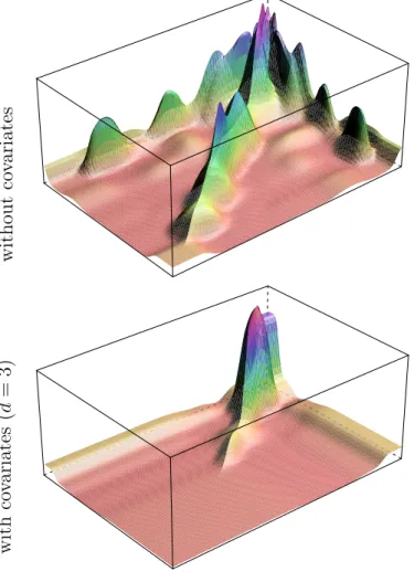
For illustration purposes, the estimation of the residual structure g ◦φˆ of this data set is provided in Figure 2 (d = 3). In practice, we used Proposition 10 to estimate ˆφ and then applied g(·) to obtain a graphon like surface. We can observe that g◦φˆis not constant for d = 3 which is coherent with H0 being rejected. Moreover, we also give in
this figure the estimated residual structure without taking the covariates into account (d= 0). Clearly, the shape ofg◦φˆis simpler whend= 3. In particular, many of the hills on the diagonal vanish when adding the covariates. Thus, the covariates help in studying and explaining parts of the network. However, they are not sufficient and some of the heterogeneity observed in the network cannot be explained by political parties and writer status.
5.2
Tree network
This data set was first introduced by [33] and further studied in [27]. We considered the tree network which describes the interactions between 51 trees where two trees in-teract if they share at least one common fungal parasite. Three covariates are available
Figure 2: Estimation of the blog network residual structure with and without covariates. without co v ar iates with co v ariates ( d = 3)
Figure 3: Estimation of the tree network residual structure with and without covariates. without co v ar iates with co v ariates ( d = 3)
characterizing the genetic, geographic, and taxonomic distances between the tree species. As for the blog network, we applied the variational algorithm for values of K between 1 and 16. For eachK, the procedure was repeated 20 times for various initializations and the best run was selected. Model H0 was rejected with a value of ˆp(H0|Y)≈ 7.5e−153
close to zero. Thus, the interactions between trees through common fungal parasite cannot be entirely explained by the distances available. This is consistent with a these from [27] who describe a residual heterogeneity in the valued version of this network, after taking the covariates into account.
Finally, we give the estimated residual structure g ◦φˆ for this data set in Figure 3 (d= 3). First, we note that the structure is not constant which is coherent withH0 being
rejected. Moreover, we also provide in this figure the estimated structure without taking the covariates into account (d = 0). Thus, as for the blog network, we find that adding the covariates induces a simplification of g◦φ. The extra diagonal holes vanish and theˆ residual structure is closer to a constant function.
6
Conclusion
In this paper we proposed a framework to assess the goodness of fit of logistic models for binary networks. Thus, we added a generic term, related to the graphon function of W-graph models, to the logistic regression model. The corresponding new model was ap-proximated with a series of models with blockwise constant residual structure. A Bayesian procedure was then considered to derive goodness-of-fit criteria. All these criteria depend on marginal likelihood terms for which we did provide estimates relying on variational approximations. The first approximation was obtained using a variational decomposition while the second involves a series of Taylor expansions. The approach was tested on toy data sets and encouraging results were obtained. Finally, it was used to analyze two real networks from social sciences and ecology. We believe the methodology has a large spec-trum of applications since logistic regression models are highly used in practice to deal with covariates in binary networks.
A
Appendix
A.1
Proof of Proposition 1
Let us start by showing that:
logp(Y|Z, α, β)≥logph(Z, α, β, ξ),
where ξ is an n×n positive real matrix. We use the bound on the log-logistic function introduced by [17] from Taylor expansions:
logg(x)≥logg(ξ) + x−ξ
2 −λ(ξ)(x
2−ξ2),∀(x, ξ)∈
R×R+, (7)
where λ(ξ) = (g(ξ)−1/2)/(2ξ). Note that (7) is an even function and therefore we can consider only positive values of x without loss of generality. Since
logp(Yij|Zi, Zj, α, β) = Yij(Zi|αZj+x|ijβ) + logg(−Z
|
iαZj−x|ijβ),
then
logp(Yij|Zi, Zj, α, β)≥Yij(Zi|αZj+x|ijβ) + logg(ξij)−
Zi|αZj +x|ijβ+ξij 2 −λ(ξij)((Zi|αZj +x|ijβ) 2−ξ2 ij) = (Yij − 1 2)(Z | iαZj+x|ijβ)− ξij 2 + logg(ξij) −λ(ξij)((Zi|αZj +x|ijβ) 2−ξ2 ij).
Note that for undirected networks, the matrixξhas to be symmetric,i.e. ξij =ξji,∀i6=j.
We then have logp(Y|Z, α, β) = 1 2 n X i6=j logp(Yij|Zi, Zj, α, β). Therefore
logp(Y|Z, α, β)≥logph(Z, α, β, ξ). Finally, LK(q) = X Z Z q(Z, π, α, β, γ, η) logp(Y, Z, π, α, β, γ, η) q(Z, π, α, β, γ, η) dπdαdβdγdη =X Z Z q(Z, π, α, β, γ, η) logp(Y|Z, α, β)p(Z, π, α, β, γ, η) q(Z, π, α, β, γ, η) dπdαdβdγdη ≥X Z Z q(Z, π, α, β, γ, η) log p h(Z, α, β, ξ)p(Z, π, α, β, γ, η) q(Z, π, α, β, γ, η) dπdαdβdγdη =LK(q; ξ).
A.2
Proof of Proposition 2
logq(Zi) = EZ\i,α,β,π 1 2logh(Z, α, β, ξ) + logp(Z|π) + cst =EZ\i,α,β,π " 1 2 n X i6=j (Yij − 1 2)Z | iαZj−λ(ξij) (Zi|αZj)2+ 2Zi|αZix|ijβ + n X i=1 Ziklogπk # + cst. Note that EZj,α[Z | iαZj] =EZj,α " K X k,l ZikαklZjl # = K X k=1 Zik ( K X l=1 (mα)klτjl ) . Furthermore EZj,α[(Z | iαZj)2] =EZj,α K X k,l ZikαklZkl !2 =EZj,α K X k,k0,l,l0 ZikZik0αklαk0l0ZjlZjl0 . (8)Because all vectorsZiare sampled from a multinomial distribution with parameters (1, π),
all terms ZikZik0 = 0 for k 6=k 0 and Z2 ik =Zik in (8). Therefore (Zi|αZj)2 = K X k,l Zikα2klZjl. (9) This leads to EZj,α[(Z | iαZj)2] = K X k=1 Zik ( K X l=1 Eαkl[α 2 kl]τjl ) . Finally logq(Zi) = K X k=1 Zik ( K X l=1 (mα)kl 1 2 n X j6=i (Yij− 1 2)−2λ(ξij)x | ijmβ τjl− K X l=1 Eαkl[α 2 kl] 1 2 n X j6=i λ(ξij)τjl + K X l=1 (mα)lk 1 2 n X j6=i (Yji− 1 2)−2λ(ξji)x | jimβ τjl− K X l=1 Eαlk[α 2 lk] 1 2 n X j6=i λ(ξji)τjl +ψ(enk)−ψ K X l=1 enl ) + cst.
Since (mα)kl= (mα)lk,Eαkl[α 2 kl] =Eαlk[α 2 lk],Yij =Yji, xij =xji, ξij =ξji, then logq(Zi) = K X k=1 Zik ( K X l=1 (mα)kl n X j6=i (Yij− 1 2)−2λ(ξij)x | ijmβ τjl− K X l=1 Eαkl[α 2 kl] n X j6=i λ(ξij)τjl +ψ(enk)−ψ K X l=1 enl ) + cst. Therefore q(Zi) =M(Zi; 1, τi), where PK k=1τik = 1 and τik ∝exp ( K X l=1 (mα)kl n X j6=i (Yij − 1 2)−2λ(ξij)x | ijmβ τjl− K X l=1 Eαkl[α 2 kl] n X j6=i λ(ξij)τjl +ψ(enk)−ψ K X l=1 enl ) .
A.3
Proof of Proposition 3
logq(π) =EZ[logp(Z|π) + logp(π)] + cst
= n X i=1 K X k=1 τiklogπk+ K X k=1 (e0−1) logπk+ cst = K X k=1 e0+ n X i=1 τik−1 logπk+ cst. Therefore q(π) = Dir(π; en), where en k =e0+Pni=1τik,∀k ∈ {1, . . . , K}.
A.4
Proof of Proposition 4
logq(β) =EZ,α,η 1 2logh(Z, α, β, ξ) + logp(β|η) + cst =EZ,α,η " 1 2 n X i6=j n (Yij −1/2)x|ijβ−λ(ξij) (x|ijβ)2+ 2Zi|αZjx|ijβ o − η 2β |β # + cst =β| ( 1 2 n X i6=j Yij − 1 2−2λ(ξij)τ | i mατj xij ) − 1 2β | ( cn dn Id+ n X i6=j λ(ξij)xijx|ij ) β+ cst.
Therefore q(β) = N(β; mβ, Sβ), where Sβ−1 = cn dn Id+ n X i6=j λ(ξij)xijx|ij, and mβ =Sβ 1 2 n X i6=j Yij − 1 2 −2λ(ξij)τ | i mατj xij.
A.5
Proof of Proposition 5
logq(γ) = Eα[logp(α|γ) + logp(γ)] + cst
=Eα " K X k≤l 1 2log(γ)− K X k≤l γ 2α 2 kl # + (a0−1) logγ−b0γ+ cst = (a0+ K(K+ 1) 4 −1) logγ− b0+ 1 2 K X k≤l Eαkl[α 2 kl] ! γ+ cst. Therefore q(γ) = Gam(γ; an, bn), where an=a0+ K(K4+1) and bn =b0+12PKk≤lEαkl[α 2 kl].
A.6
Proof of Proposition 6
logq(η) =Eβ[logp(β|η) + logp(η)] + cst
=Eβ d 2logη− η 2β |β + (c0 −1) logη−d0η+ cst = (c0+ d 2 −1) logη−(d0+ 1 2Tr(Sβ) + 1 2m | βmβ)η+ cst. Therefore q(η) = Gam(η; cn, dn), where cn =c0+d2 and dn=d0+ 12Tr(Sβ) + 12m|βmβ.
A.7
Proof of Proposition 7
logq(α) =EZ,β,γ 1 2logh(Z, α, β, ξ) + logp(α|γ) + cst =EZ,β,γ " 1 2 n X i6=j (Yij − 1 2)Z | iαZj−λ(ξij) (Zi|αZj)2+ 2Zi|αZjx|ijβ − K X k≤l γ 2α 2 kl # + cst. (10)We have Zi|αZj = PKk,lZikαklZkl and (Zi|αZj)2 = PKk,lZikαkl2 Zkl = Zi|AZj (see Eq. 9)
with A the K ×K matrix such that Akl = αkl2. Moreover, any expression of the form
(1/2)Pn
i6=jcijZ
|
iBZj where B is a symmetric K×K matrix and cij =cji can be written
1 2 n X i6=j cijZi|BZj = 1 2 n X i6=j cij K X k,l ZikBklZjl = 1 2 n X i6=j cij K X k=1 ZikBkkZjk + K X k<l ZikBklZjl+ K X k<l ZjkBlkZil ! = K X k=1 Bkk 1 2 n X i6=j cijZikZjk + K X k<l Bkl 1 2 n X i6=j cijZikZjl+ 1 2 n X i6=j cijZjkZil ! . By exchanging the role ofiand j in the sum of the last term and sincecij =cji, we obtain
1 2 n X i6=j cijZi|BZj = K X k=1 Bkk 1 2 n X i6=j cijZikZjk+ K X k<l Bkl n X i6=j cijZikZjl. (11) Using (11) in (10) leads to logq(α) = K X k=1 αkk n X i6=j 1 2(Yij − 1 2)−λ(ξij)x | ijmβ τikτjk + K X k<l αkl n X i6=j (Yij − 1 2)−2λ(ξij)x | ijmβ τikτjl − K X k=1 α2kk n X i6=j 1 2λ(ξij)τikτjk − K X k<l α2kl n X i6=j λ(ξij)τikτjl − K X k≤l an 2bn α2kl. Therefore q(α) = K Y k6=l N αkl; (mα)kl,(σ2α)kl ,
where (σ2α)−kk1 = an bn + n X i6=j λ(ξij)τikτjk,∀k, (σ2α)−kl1 = an bn + 2 n X i6=j λ(ξij)τikτjl,∀k6=l, (mα)kk = (σα2)kk n X i6=j 1 2(Yij − 1 2)−λ(ξij)x | ijmβ τikτjk (mα)kl = (σα2)kl n X i6=j (Yij − 1 2)−2λ(ξij)x | ijmβ τikτjl.
A.8
Proof of Proposition 9
LK(q;ξ) = EZ,π,α,β,γ,η
h
logph(Z, α, β, ξ) + logp(Z, π, α, β, γ, η)i−EZ,π,α,β,γ,η[logq(Z, π, α, β, γ, η)]
LK(q; ξ) = 1 2 n X i6=j ( (Yij − 1 2)(EZi,Zj,α[Z | iαZj] +x|ijEβ[β]) + logg(ξij)− ξij 2 −λ(ξij) EZi,Zj,α[(Z | iαZj)2] + 2EZi,Zj,α[Z | iαZj]x|ijEβ[β] +Eβ[(x|ijβ) 2]−ξ2 ij ) + n X i=1 K X k=1
EZi[Zik]Eπ[logπk]−logC(e) +
K X k=1 (e0−1)Eπ[logπk]− K(K+ 1) 4 log(2π) + K(K+ 1) 4 Eγ[logγ]− Eγ[γ] 2 K X k≤l Eαkl[α 2 kl]− d 2log(2π) + d 2Eη[logη]− Eη[η] 2 Eβ[β |β]
−log Γ(a0) +a0logb0 + (a0−1)Eγ[logγ]−b0Eγ[γ]−log Γ(c0)
+c0logd0+ (c0−1)Eη[logη]−d0Eη[η]− n X i=1 K X k=1
EZi[Zik] logτik+ logC(e
n) − K X k=1 (enk −1)Eπ[logπk] + K(K+ 1) 4 log(2π) + 1 2 K X k≤l log(σα2)kl+ 1 2 K X k≤l (σα2)−kl1Eαkl[α 2 kl] − K X k≤l (σα2)−kl1Eαkl[αkl](mα)kl+ 1 2 K X k≤l (σ2α)−kl1(mα)2kl+ d 2log(2π) + 1 2log|Sβ| + 1 2Eβ[β |S−1 β β]−Eβ[β]|Sβ−1mβ + 1 2mβS −1
β mβ+ log Γ(an)−anlogbn
−(an−1)Eγ[logγ] +bnEγ[γ] + log Γ(cn)−cnlogdn−(cn−1)Eη[logη]
whereC(x) =
QK k=1Γ(xk)
Γ(PK
k=1xk) and Γ(·) is the gamma function. The terms inEγ[logγ],Eη[logη],
Eπ[logπ] and log(2π) do simplify in (12) after the VBEM update step. This leads to
LK(q; ξ) = 1 2 n X i6=j ( (Yij − 1 2)(EZi,Zj,α[Z | iαZj] +x|ijEβ[β]) + logg(ξij)− ξij 2 −λ(ξij) EZi,Zj,α[(Z | iαZj)2] + 2EZi,Zj,α[Z | iαZj]x|ijEβ[β] +Eβ[(x|ijβ) 2 ]−ξij2 ) −logC(e)− an 2bn K X k≤l Eαkl[α 2 kl]− cn 2dn Tr(Sβ +mβm|β)
−log Γ(a0) +a0logb0−b0
an bn −log Γ(c0) +c0logd0−d0 cn dn − n X i=1 K X k=1
τiklogτik+ logC(en) +
1 2 K X k≤l log(σ2α)kl+ 1 2 K X k≤l (σ2α)−kl1Eαkl[α 2 kl] −1 2 K X k≤l (σ2α)−kl1(mα)2kl+ 1 2log|Sβ|+ 1 2Tr S −1 β (Sβ+mβ(mβ)|) − 1 2m | βS −1
β mβ+ log Γ(an)−anlogbn+bn
an bn + log Γ(cn) −cnlogdn+dn cn dn . Moreover, using (11), note that
1 2 n X i6=j (Yij − 1 2)EZi,Zj,α[Z | iαZj] = K X k=1 Eαkk[αkk] 1 2 n X i6=j (Yij − 1 2)τikτjk + K X k<l Eαkl[αkl] n X i6=j (Yij − 1 2)τikτjl, 1 2 n X i6=j 2λ(ξij)EZi,Zj,α[Z | iαZj]x|ijEβ[β] = K X k=1 Eαkk[αkk] n X i6=j λ(ξij)x|ijEβ[β]τikτjk + K X k<l Eαkl[αkl]2 n X i6=j λ(ξij)x|ijEβ[β]τikτjl.
Using (9) and (11), 1 2 n X i6=j λ(ξij)EZi,Zj,α[(Z | iαZj)2] = K X k=1 Eαkk[α 2 kk] 1 2 n X i6=j λ(ξij)τikτjk + K X k<l Eαkl[α 2 kl] n X i6=j λ(ξij)τikτjl Finally Eβ[(x|ijβ) 2 ] =Eβ x|ijβx|ijβ =Eβ x|ijββ|xij = Tr xijx|ijEβ[ββ|] = Tr xijx|ij(Sβ+mβm|β) . Therefore LK(q; ξ) = 1 2 n X i6=j logg(ξij)− ξij 2 +λ(ξij)ξ 2 ij + logC(e n) C(e) + log Γ(an) Γ(a0) + logΓ(cn) Γ(c0) +a0logb0+an(1− b0 bn −logbn) +c0logd0+cn(1− d0 dn −logdn) +1 2 K X k≤l log(σα2)kl+ 1 2log|Sβ| − n X i=1 K X k=1 τiklogτik− 1 2 K X k≤l (σ2α)−kl1(mα)2kl− 1 2m | βS −1 β mβ + K X k=1 (mα)kk n X i6=j 1 2(Yij − 1 2)−λ(ξij)x | ijmβ τikτjk + K X k<l (mα)kl n X i6=j (Yij − 1 2)−2λ(ξij)x | ijmβ τikτjl − K X k=1 Eαkk[α 2 kk] 1 2 an bn −(σ2α)−kk1+ n X i6=j λ(ξij)τikτjk ! − K X k<l Eαkl[α 2 kl] 1 2 an bn −(σ2α)−kl1+ 2 n X i6=j λ(ξij)τikτjl ! +1 2m | β n X i6=j (Yij− 1 2)xij −1 2Tr 2 n X i6=j λ(ξij)xijx|ij + cn dn Id−Sβ−1 (Sβ+mβm|β) ! .
Finally, since the terms at the fourth and fifth line correspond exactly toPK
k≤l(mα)kl(σα2)
−1
kl (mα)kl,
and after the VBEM update step
LK(q; ξ) = 1 2 n X i6=j logg(ξij)− ξij 2 +λ(ξij)ξ 2 ij + logC(e n) C(e) + log Γ(an) Γ(a0) + logΓ(cn) Γ(c0) +a0logb0+an(1− b0 bn −logbn) +c0logd0+cn(1− d0 dn −logdn) +1 2 K X k≤l log(σα2)kl+ 1 2log|Sβ| − n X i=1 K X k=1 τiklogτik+ 1 2 K X k≤l (σ2α)−kl1(mα)2kl− 1 2m | βS −1 β mβ +1 2m | β n X i6=j (Yij− 1 2)xij.
A.9
Proof of Proposition 8
Keeping only the terms that do depend on ξij in (12), the lower bound is given by
LK(q; ξ) = 1 2 n X i6=j ( logg(ξij)− ξij 2 −λ(ξij) EZi,Zj,α[(Z | iαZj)2] + 2EZi,Zj,α[Z | iαZj]x|ijEβ[β] +Eβ[(x|ijβ) 2]−ξ2 ij ) + cst = 1 2 n X i6=j ( logg(ξij)− ξij 2 −λ(ξij) XK k,l τikτjlEαkl[α 2 kl] + 2 K X k,l τikτjl(mα)klx|ijmβ + Tr(xijx|ij(Sβ +mβm|β))−ξij2 ) + cst.
The partial derivative of the lower bound with respect to ξij is
∂LK ∂ξij (q; ξ) = g(−ξij)− 1 2 −λ 0 (ξij) XK k,l τikτjlEαkl[α 2 kl] + 2 K X k,l τikτjl(mα)klx|ijmβ + Tr(xijx|ij(Sβ +mβm|β))−ξ 2 ij + 2λ(ξij)ξij, and ∂LK ∂ξij (q; ξ) = −λ0(ξij) XK k,l τikτjlEαkl[α 2 kl] + 2 K X k,l τikτjl(mα)klx|ijmβ + Tr(xijx|ij(Sβ+mβm|β))−ξij2 . (13)
Finally, λ(ξij) is a strictly decreasing function for positive values ofξij . Thus, λ 0
(ξij)6= 0
and therefore if we set (13) to zero, we obtain
ξij2 = K X k,l τikτjlEαkl[α 2 kl] + 2 K X k,l τikτjl(mα)klx|ijmβ + Tr(xijx|ij(Sβ +mβm|β)). Note thatξij =ξji.
References
[1] Edoardo M Airoldi, Thiago B Costa, and Stanley H Chan. Stochastic blockmodel approximation of a graphon: Theory and consistent estimation. In Advances in
Neural Information Processing Systems, pages 692–700, 2013.
[2] R. Albert and A.L. Barab´asi. Statistical mechanics of complex networks. Modern
Physics, 74:47–97, 2002.
[3] D. Asta and C. R. Shalizi. Geometric network comparison. Technical report, arXiv:1411.1350v1, 2014.
[4] A.L. Barab´asi and Z.N. Oltvai. Network biology: understanding the cell’s functional organization. Nature Rev. Genet, 5:101–113, 2004.
[5] M.J. Beal and Z. Ghahramani. The variational bayesian em algorithm for incom-plete data: with application to scoring graphical model structures. In JM Bernardo, MJ Bayarri, JO Berger, AP Dawid, D Heckerman, AFM Smith, and M (eds) West, editors,Bayesian Statistics 7: Proceedings of the 7th Valencia International Meeting, page 453, 2002.
[6] C.M. Bishop. Pattern recognition and machine learning. Springer-Verlag, 2006. [7] C.M. Bishop and M. Svens´en. Bayesian hierarchical mixtures of experts. In
Proceed-ings of the 19th Conference on Uncertainty in Artificial Intelligence, pages 57–64. U.
Kjaerulff and C. Meek, 2003.
[8] F. Caron and A. Doucet. Sparse bayesian nonparametric regression. In Proceedings
of the 25th International Conference on Machine Learning, 2008.
[9] S. Chatterjee. Matrix estimation by Universal Singular Value Thresholding. The
Annals of Statistics, 43(1):177–214, 2015.
[10] A.P. Dempster, N.M. Laird, and D.B. Rubin. Maximum likelihood for incomplete data via the em algorithm. Journal of the Royal Statistical Society, B39:1–38, 1977. [11] P. Diaconis and S. Janson. Graph limits and exchangeable random graphs. Rend.
[12] C. Ducruet. Network diversity and maritime flows. Journal of Transport Geography, 30:77–88, 2013.
[13] A. Goldenberg, A.X. Zheng, S.E. Fienberg, and E.M. Airoldi. A survey of statistical network models. Foundations and Trends in Machine Learning, 2(2):129–233, 2010. [14] Mark S Handcock, Adrian E Raftery, and Jeremy M Tantrum. Model-based clustering for social networks. Journal of the Royal Statistical Society: Series A (Statistics in
Society), 170(2):301–354, 2007.
[15] P.D. Hoff. Modeling homophily and stochastic equivalence in symmetric relational data. In Advances in Neural Information Processing Systems, pages 657–664, 2008. [16] Peter D Hoff, Adrian E Raftery, and Mark S Handcock. Latent space approaches to
social network analysis.Journal of the american Statistical association, 97(460):1090– 1098, 2002.
[17] T.S. Jaakkola and M.I. Jordan. Bayesian parameter estimation via variational
meth-ods. Statistics and Computing, 10:25–37, 2000.
[18] H. Jeffreys. An invariant form for the prior probability in estimations problems. In
Proceedings of the Royal Society of London. Series A, volume 186, pages 453–461,
1946.
[19] Y. Jernite, P. Latouche, C. Bouveyron, P. Rivera, L. Jegou, and S. Lamass´e. The random subgraph model for the analysis of an acclesiastical network in merovingian gaul. Annals of Applied Statistics, 8(1):377–405, 2014.
[20] O. Kallenberg. Multivariate sampling and the estimation problem for exchangeable arrays. Journal of Theoretical Probability, 12(3):859–883, 1999.
[21] R. E Kass and A. E Raftery. Bayes factors. Journal of the american statistical
association, 90(430):773–795, 1995.
[22] V. Lacroix, C.G. Fernandes, and M.-F. Sagot. Motif search in graphs:application to metabolic networks. Transactions in Computational Biology and Bioinformatics, 3:360–368, 2006.
[23] P. Latouche, E Birmel´e, and C. Ambroise. Overlapping stochastic block models with application to the french political blogosphere. Annals of Applied Statistics, 5(1):309–336, 2011.
[24] P. Latouche, E Birmel´e, and C. Ambroise. Model selection in overlapping stochastic block models. Electronic Journal of Statistics, 8(1):762–794, 2014.
[25] P. Latouche and S Robin. Bayesian model averaging of stochastic block models to estimate the graphon function and motif frequencies in a W-graph model. Technical report, arXiv:1310.6150, 2013.
[26] L. Lov´asz and B. Szegedy. Limits of dense graph sequences. Journal of Combinatorial
Theory, Series B, 96(6):933 – 957, 2006.
[27] M. Mariadassou, S. Robin, and C. Vacher. Uncovering latent structure in valued graphs: a variational approach. Annals of Applied Statistics, 4(2), 2010.
[28] C. Matias and S. Robin. Modeling heterogenity in random graphs through latent space models: a selective review. Esaim Prooceedings and Surveys, 47:55–74, 2014. [29] Mark E. J. Newman. The structure and function of complex networks. SIAM Review,
45:167–256, 2003.
[30] K. Nowicki and T.A.B. Snijders. Estimation and prediction for stochastic blockstruc-tures. Journal of the American Statistical Association, 96:1077–1087, 2001.
[31] G. Palla, L. Lovasz, and T. Vicsek. Multifractal network generator. Proc. Natl. Acad.
Sci. U.S.A., 107(17):7640–7645, Apr 2010.
[32] T.A.B. Snijders and K. Nowicki. Estimation and prediction for stochastic block-structures for graphs with latent block structure.Journal of Classification, 14:75–100, 1997.
[33] C. Vacher, D. Piou, and M.-L. Desprez-Loustau. Architecture of an antagonistic tree/fungus network: The asymmetric influence of past evolutionary history. PLoS ONE, 3(3):1740, 2008. e1740. doi:10.1371/journal.pone.0001740.
[34] N. Villa, F. Rossi, and Q.D. Truong. Mining a medieval social network by kernel som and related methods. Arxiv preprint arXiv:0805.1374, 2008.
[35] Stevenn Volant, Marie-Laure Martin Magniette, and St´ephane Robin. Variational bayes approach for model aggregation in unsupervised classification with markovian dependency. Comput. Statis. & Data Analysis, 56(8):2375 – 2387, 2012.
[36] Y.J. Wang and G.Y. Wong. Stochastic blockmodels for directed graphs. Journal of
the American Statistical Association, 82:8–19, 1987.
[37] D.J. Watts and S.H. Strogatz. Collective dynamics of small-world networks. Nature, 393:440–442, 1998.
[38] P. J. Wolfe and S. C. Olhede. Nonparametric graphon estimation. Technical report, arXiv:1309.5936, 2013.
[39] H. Zanghi, C. Ambroise, and V. Miele. Fast online graph clustering via erd¨os-r´enyi mixture. Pattern Recognition, 41(12):3592–3599, 2008.
[40] H. Zanghi, S. Volant, and C. Ambroise. Clustering based on random graph model embedding vertex features. Pattern Recognition Letters, 31(9):830–836, 2010.