Turbulent drag reduction using surface plasma

(1)

Jukes, Timothy N. (2007) Turbulent drag reduction using

surface plasma. PhD thesis, University of Nottingham.

Access from the University of Nottingham repository: http://eprints.nottingham.ac.uk/12160/1/490832.pdf

Copyright and reuse:

The Nottingham ePrints service makes this work by researchers of the University of Nottingham available open access under the following conditions.

· Copyright and all moral rights to the version of the paper presented here belong to the individual author(s) and/or other copyright owners.

· To the extent reasonable and practicable the material made available in Nottingham ePrints has been checked for eligibility before being made available.

· Copies of full items can be used for personal research or study, educational, or not-for-profit purposes without prior permission or charge provided that the authors, title and full bibliographic details are credited, a hyperlink and/or URL is given for the original metadata page and the content is not changed in any way.

· Quotations or similar reproductions must be sufficiently acknowledged.

Please see our full end user licence at:

http://eprints.nottingham.ac.uk/end_user_agreement.pdf

A note on versions:

The version presented here may differ from the published version or from the version of record. If you wish to cite this item you are advised to consult the publisher’s version. Please see the repository url above for details on accessing the published version and note that access may require a subscription.

(2)

TURBULENT DRAG REDUCTION USING

SURFACE PLASMA

Timothy N. Jukes, MEng.

T

HESIS SUBMITTED TO THE

U

NIVERSITY OF

N

OTTINGHAM

FOR THE DEGREE OF

D

OCTOR OF

P

HILOSOPHY

(3)

Abstract

An experimental investigation has been undertaken in a wind tunnel to study the induced airflow and drag reduction capability of AC glow discharge plasma actuators.

Plasma is the fourth state of matter whereby a medium, such as air, is ionized creating a system of electrons, ions and neutral particles. Surface glow discharge plasma actuators have recently become a topic for flow control due to their ability to exert a body force near the wall of an aerodynamic object which can create or alter a flow. The exact nature of this force is not well understood, although the current state of knowledge is that the phenomenon results from the presence of charged plasma particles in a highly non-uniform electric field. Such actuators are lightweight, fully electronic (needing no moving parts or complicated ducting), have high bandwidth and high energy density. The manufacture of plasma actuators is relatively cheap and they can be easily retrofitted to existing surfaces.

The first part of this study aims at characterising the airflow induced by surface plasma actuators in initially static air. Ambient air temperature and velocity profiles are presented around a variety of actuators in order to understand the nature of the induced flow for various parameters such as applied voltage, frequency, actuator geometry and material. It is found that the plasma actuator creates a laminar wall jet along the surface of the material on which it is placed.

The second part of the study aims at using plasma actuators to reduce skin-friction drag in a fully developed turbulent boundary layer. Actuators are

(4)

designed to induce spanwise forcing near the wall, oscillating in time. Thermal anemometry measurements within the boundary layer are presented. These show that the surface plasma can cause a skin-friction drag reduction of up to 45% due to the creation of streamwise vortices which interact with, and disrupt the near-wall turbulence production cycle.

(5)

Acknowledgements

I am indebted to my supervisor, Prof. Kwing-So Choi, for his support, helpful suggestions and encouragement during the course of this study. I would also like to extend my thanks to Dr. Graham Johnson and Dr. Simon Scott from BAE SYSTEMS, UK, for useful advice, the loan of the plasma equipment and for co-funding the project. Thanks are given to the EPSRC for project funding and for the loan of the thermal camera. Also, thanks are extended to Dr. Takehiko Segawa and Dr. Hiro Yoshida from the National Institute of Advanced Industrial Science and Technology, Japan, for their useful discussions and providing the ceramic samples.

Thanks must go to my colleagues Dr. Faycal Bahri, Yang Xu, Peng Xu and Yong-Duck Kang for their support and suggestions over the years. I would especially like to thank Tracey for her patience and support, especially whilst writing this thesis, and to Mum and Dad.

(6)

5.3.1. Induced Flow Field – Steady State 165 5.3.2. Induced Flow Field – Flow Initiation 171 5.3.3. Effect of Plasma Parameters 179 5.3.3.1. Effect of the Excitation Voltage, E 180 5.3.3.2. Effect of the Pulse Repetition Frequency, PRF 185 5.3.3.3. Effect of the Pulse Envelope Duration, PED 187 5.3.3.4. Effect of the Pulse Envelope Frequency, PEF 189 5.3.3.5. Velocity Variation with Applied Power 191

5.4. Effect of Dielectric Material 193

5.4.1. 600ȝm Si3N4Ceramic Actuator 197

5.4.2. Parametric Testing of Ceramic Actuators 203 Chapter 6. Measurement of Plasma Temperature 207

6.2. Thermal Camera Operating Principles 207

6.3. Equipment Set-up 212

6.4. Thermal Reflections 214

(9)

6.5.1. Sensitivity Analysis 217

6.6. Results 218

6.6.1. One-Dimensional Analysis 218

6.6.2. Estimation of Plasma Temperature, Tplasma 221 6.6.3. Surface Temperature with Pulsed Plasma 225

Chapter 7. Plasma Induced Wall Normal Jets 230

7.2. Velocity Measurements and Flow Visualisation 231 Chapter 8. Spanwise Oscillation Electrode Sheets 237

8.2. Electrode Sheet Design 238

8.2.1. Operating Principle 238

8.2.2. End Effects 245

8.3. Visualisation of Spanwise Oscillation Actuators in Still Air 249 Chapter 9. Plasma Effect on the Turbulent Boundary Layer 254

9.2. Drag Measurement and Scaling 255

9.2.1. Skin Friction Measurement and Wall Positioning 255

9.2.2. Outer Scaling 258

9.3. Thermal Boundary Layer 260

9.4. Momentum Boundary Layer 267

9.4.1.U-component Velocity 267

9.4.2.UV and UW Component Measurements 276

9.4.3. Energy Spectra and PDF 287

(10)

9.4.5. VITA Events With and Without Plasma 297 9.4.6. Phase-Averaged Spanwise Velocity 304

9.4.7. Spanwise Variation 308

9.5. Summary 311

Chapter 10. Parametric Effects 321

10.1. Effect of Oscillation Period, T+ 321

10.2. Effect of Electrode Spacing, s 327 10.3. Effect of Pulse Envelope Duration, PED 332 Chapter 11. Conclusions and Future Recommendations 336

11.2. Plasma Actuators in Initially Static Air 336 11.3. Spanwise Oscillation Plasma for Drag Reduction 341

11.4. Summary 346

11.5. Future recommendations 347

References 349

Appendix

Jukes, T. N., Choi, K.-S., Johnson, G. A., Scott, S. J., 2006, “Characterisation of Surface Plasma Induced Wall Flows through Velocity and Temperature Measurement”,AIAA J.,44, No.4, pp. 764-771. 368

(11)

Nomenclature

A calibration constant

a hot-wire heating ratio (Rw/Ra); electrode spacing

B magnetic induction tensor

B calibration constant

B0 magnetic field strength at wall

C capacitance; calibration constant

c chord length

cf skin-friction coefficient

D electric induction tensor

D VITA detector function; calibration constant

d distance between electrodes; hot-wire diameter

E electric field tensor

E voltage EB breakdown voltage e electron change F calibration constant f oscillation frequency fb body force fc cut-off frequency Gr Grasshof number (gȕ(T - T)l3/Ȟ) g gravitational acceleration

H magnetic field strength tensor

H shape factor (į*/ș)

h channel half-height; heat transfer coefficient

I current

j current density tensor

k thermal conductivity; VITA detector threshold; Boltzmann constant

l reference length

me electron mass

mi ion mass

(12)

P power

p pressure

PED Pulse Envelope Duration

PEF Pulse Envelope Frequency

PRF Pulse Repetition Frequency

Q Flow rate

q charge

R molar gas constant

Ra resistance of wire at ambient temperature, Ta

Rc cable resistance

Rl lead resistance

Rx(Ĳ) autocorrelation function

Rw resistance of heated wire at temperature, Tw

Re_į Reynolds number of wall jet (Umaxį½/Ȟ)

Reș momentum thickness Reynolds number (Uș/Ȟ)

ReĲ friction velocity Reynolds number (u*į/Ȟ)

r radial distance

St Stuart number (J0B0į/ȡu*2)

s electrode spacing

T temperature; oscillation period

Ta,T ambient temperature Te electron temperature

Tens VITA ensembling window length

TI integral time scale

Ti ion temperature

Tw temperature of heated wire

Twin window length

tanį dielectric loss tangent

t time

tAC plasma repetition period (2/PRF)

U mean streamwise velocity

U free-stream velocity

Umax maximum wall-jet velocity

(13)

u* friction velocity

u’ streamwise turbulence intensity

V mean wall-normal velocity

v’ wall-normal turbulence intensity

vc particle collision frequency

W mean spanwise velocity; radiation power

W+ non-dimensional wall speed (ʌ.ǻz+/T+)

Weq+ equivalent non-dimensional wall speed (St.T+/(2ʌ.ReĲ))

w’ spanwise turbulence intensity

x streamwise direction

y wall-normal direction

z spanwise direction

ǻz+ non-dimensional wall-oscillation amplitude

Į phase angle; coefficient of resistivity; spectral absoptance;

thermal diffusivity

ȕ thermal expansion coefficient; yaw angle ǻ change in a quantity

ǻ thermal boundary layer thickness ǻ+ _{non-dimensional penetration depth (}

au*/ʌȞ)

į boundary layer thickness į*

displacement thickness

<½ wall-jet half-width

İ dielectric constant; spectral emissivity İ0 permittivity of free space

ș momentum thickness; pitch angle

Ȝ wavelength

ȜD Debye length

ȝ dynamic viscosity Ȟ kinematic viscosity (ȝ/ȡ) ȡ density; spectral reflectance ȡc charge density

ȡx(Ĳ) autocorrelation coefficient function

Ĳ shear stress; spectral transmittance; time delay Ĳw mean wall shear stress (skin-friction)

(14)

ĳ electric potential Ȧ vorticity; angular velocity

Subscripts and Superscripts

+ indicates viscous scaling, also referred to as inner-scaling. Viscous time, length and velocity scales are t+ = tu*2/Ȟ,l+= lu*/Ȟ,u+ = U/u* ̅ indicates wall-jet scaling with local maximum velocity, Umax, and jet

half-width,<½. Time, length and velocity scales are t̅ = tUmax/<½,l̅ =

l/<½,U̅ = U/Umax ’ rms value #1, #2 wires 1 and 2 0 value at 0C; value at y = 0 free-stream condition w value at wall

ensemble-averaged quantity (in this case streamwise velocity)

u time-averaged quantity

(15)

List of Tables

2.2.1 Quadrant definitions of Reynolds stress from Wallace et al. (1972) 11

5.3.1 Details of Mylar plasma actuators 163

5.4.1 Comparison of dielectric material properties 195 6.3.1 Thermal camera close-up lens optics data 213 6.5.1 Emissivity calibration of the Mylar/copper laminate 216 6.5.2 Sensitivity of İMylar on reflected and sheet temperature readings 217 9.4.1 Near-wall velocity gradient, skin-friction coefficient, boundary layer

integral quantities, and drag reduction with and without spanwise

oscillatory plasma forcing 271

9.4.2 Change in mean velocity, normal stress and shear stress due to

oscillatory spanwise plasma forcing in a turbulent boundary layer 288 9.4.3 Boundary layer quantities and drag change with z 310 10.1.1 Drag reduction / increase caused by plasma oscillation frequency 324 10.2.1 Boundary layer quantities and drag change with s 329 10.3.1 Boundary layer quantities and drag change with PED 333

(16)

List of Figures

2.2.1 Flow visualisation at y+ = 4.5 from Kline et al. (1967) 7 2.2.2 Mechanism of streak lift up and ejection from Kline et al. (1967) 9 2.2.3 VITA ‘burst’ event from Blackwelder and Kaplan (1976) 14 2.2.4 Outer boundary layer structure from Falco (1977) 16 2.2.5 Hairpin vortex schematic from Theodorsen (1952) 19 2.2.6 Re no. effect on hairpins from Head and Bandyopadhyay (1981) 20 2.2.7 Parts of a horseshoe vortex as defined by Robinson (1991b) 20 2.2.8 Conceptual QSV and hairpin model from Robinson (1991b) 21 2.2.9 Schematic of a hairpin vortex from Adrian et al. (2000) 21 2.2.10 Conceptual model of hairpin packets from Adrian et al. (2000) 23 2.2.11 Auto-generation of a hairpin packet from Zhou et al. (1999) 27 2.2.12 Conceptual burst cycle model from Choi (1989, 2001) 28 2.2.13 Self-sustaining process of near-wall turbulence from Kim (2005) 28 2.3.1 Drag reduction for spanwise oscillation DNS of Jung et al. (1992) 33 2.3.2 Turbulence structure due to wall oscillation from Jung et al. (1992) 34 2.3.3 RMS profiles for wall oscillation from Laadhari et al. (1994) 36 2.3.4 Energy balance for wall oscillation of Baron and Quadrio (1996) 36 2.3.5 Near-wall velocity profile from Choi et al. (1998) 39 2.3.6 Streamwise variation of drag reduction from Choi et al. (1998) 39 2.3.7 Drag vs frequency and amplitude from Choi et al. (1998) 39 2.3.8 Conceptual model for a turbulent boundary layer over

an oscillating wall from Choi et al.(1998) 40 2.3.9 VITA near-wall burst signature from Choi and Clayton (2001) 41 2.3.10 w+ profile over an oscillating wall from Choi (2002) 42 2.3.11 ȍz+ created due to wall oscillation from Choi (2002) 43 2.3.12 Drag reduction vs nondimensional wall velocity, from Choi (2002) 43 2.3.13 Evolution of QSVs with spanwise wall oscillation from

Dhanak and Si (1999) 45

2.3.14 Drag reduction rate from Choi et al. (2002) 48 2.3.15 Drag reduction against T+ and Wm+from Quadrio and Ricco (2004) 48 2.3.16 Drag reduction versus S+ from Quadrio and Ricco (2004) 48 2.3.17 EMTC actuator modelled from Pang et al. (2004) 51 2.3.18 Contours of streamwise vorticity with spanwise Lorentz forcing

from Berger et al. (2000) 51

2.3.19 Drag reduction using Lorentz force vs St and T+ (Pang et al. 2004) 53 2.3.20 Skin-friction drag reduction vs Weq+. From Pang et al. (2004) 53 2.3.21 Lorentz forcing velocity profile from Breuer et al. (2004) 53 2.4.1 V-I characteristics of a DC low pressure electrical discharge

tube from Roth (1995) 56

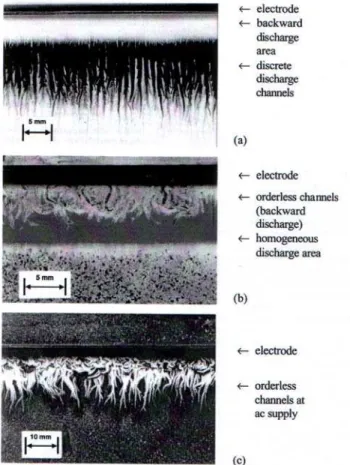
2.4.2 Parallel plate OAUGDP geometry. Adapted from Roth (2001a) 59 2.4.3 Schematic of DBD configurations from Kogelshatz et al. (1997) 61 2.4.4 Illustration of the operation of a DBD from Enloe et al. (2004b) 62 2.4.5 Discharge patterns on a DBD from Gibalov and Pietsch (2000) 63 2.4.6 CCD photographs of the plasma on a DBD from Wilkinson (2003) 64 2.4.7 Induced plasma motion by two tilted electrodes (Roth, 2001b) 66 2.4.8 Schematic of symmetric and asymmetric plasma actuators 69

(17)

2.4.9 Demonstration of plasma forcing in still air from Roth et al. (1998) 69 2.4.10 Plasma induced flow velocity in still air from Roth et al. (1998) 69 2.4.11 Electric potential for the plasma actuator geometry without and

with plasma. From Enloe et al. (2004a) 73 2.4.12 Measured flow field induced by an asymmetric plasma actuator

from Corke et al. (2002) 73

2.4.13 Effect of the frequency on the induced flow around a single

symmetric actuator in static air. From Johnson and Scott (2001) 76 2.4.14 Effect of the forcing duration on the induced flow around a

single actuator in static air. From Johnson and Scott (2001) 76 2.4.15 Induced velocity vs applied voltage from Corke and Post (2005) 76 2.4.16 Formation of counter-rotating vortices by a single streamwise

plasma electrode. From Roth et al.(1998) 78 2.4.17 Velocity profile downstream of symmetric streamwise

plasma electrodes. From Roth et al. (1998) 78 2.4.18 Leading edge vortices control from Johnson and Scott (2001) 79 2.4.19 Flow reattachment with plasma from Corke et al. (2004) 81 2.4.20 Induced velocity around a pair of plasma electrodes with

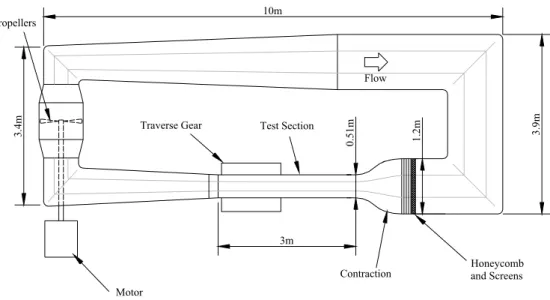
oscillatory plasma formation. From Wilkinson (2003) 82 3.2.1 Schematic of the closed return wind tunnel 85

3.2.2 Cross section of test section 85

3.3.1 Probe types used during experiments 88

3.3.2 Calibration of the cold wire probe 90

3.4.1 Optimisation of hotwire for a square wave test 91

3.4.2 Effect of hotwire probe yaw angle 97

3.4.3 Hotwire calibration curve fits 98

3.4.4 Variation in free stream velocity across the test section 99 3.4.5 Variation in temperature across the test section 100 3.6.1 Autocorrelation function and integral time scale at y+ = 15 103 3.6.2 Power spectrum at various positions in the boundary layer 104 3.6.2 Running average velocity at y+= 15 104 3.7.1 Schematic of plasma excitation parameters 107 3.7.2 Plasma electrode sheet cross section schematic 108

3.7.3 Detail of test plate 110

3.8.1 Schematic of experimental configuration 113 4.2.1 Plasma electrode sheet cross section schematic 116 4.2.2 Coordinate system and probe orientation 117 4.2.3 Photograph of electrode sheet and hot wire in the wind tunnel 117 4.2.4 Hotwire and Signal Generator A signal at x = 4mm, y = 1mm 119

4.2.5 Data processing procedure 120

4.3.1 Voltage and current waveforms 121

4.3.2 Hot-wire signals around the symmetric electrode 124 4.3.3 Hot-Wire signal at y = 1mm, x= 8mm 125 4.3.4 Variation of maximum phase-averaged velocity with PRF 128 4.3.5 Variation of maximum phase-averaged velocity with PEF 128 4.3.6 Variation of maximum phase-averaged velocity with PED 128 4.3.7 Variation of maximum phase-averaged velocity with Emax 129 4.3.8 Variation in maximum phase-averaged velocity with power 130

(18)

4.3.9 Phase-averaged velocity contours around a symmetric electrode 131 4.3.10 Velocity profiles on either side of the symmetric electrode 133

4.3.11 Non-dimensional velocity profile 133

4.3.12 Pulse-averaged velocity contours around a single electrode 134 4.3.13 Flow visualization images around the symmetric plasma electrode 135

4.3.14 Development of the wall jet 137

4.3.15 Variation of parameters with distance from electrode centreline 137 4.3.16 Phase-averaged temperature contours around an electrode 138 4.3.17 Pulse-averaged temperature contours around an electrode 139 4.3.18 Pulse-averaged temperature profiles 140 4.4.1 Hotwire signal during 1s of continuous plasma forcing 145 4.4.2 Hotwire signal during 1s of pulsed plasma forcing 145 4.4.3 Variation of U with Emax for continuous plasma forcing 148 4.4.4 Variation of U with PRF for continuous plasma forcing 148 4.5.1 Theoretical laminar wall jet flow from Tetervin (1948) 152 4.5.2 Wall jet flow angle from Tetervin (1948) 152 4.5.3 Theoretical laminar wall jet vector plot 153 4.5.4 Effective velocity sensed by the hotwire and hotwire error 153 4.5.5 Computed laminar wall jet profile at x = 4 ±0.2mm 155 5.2.1 Variation of İ with temperature for Mylar 161 5.2.2 Variation of tanį with temperature for Mylar 161

5.3.1 125ȝm thick Mylar electrode sheet 164

5.3.2 125ȝm thick Mylar electrode sheet during testing 164 5.3.3 Time-averaged velocity contours around the Mylar actuators 166 5.3.4 Time-averaged velocity profile around the Mylar actuators 167 5.3.5 Time-averaged vorticity contours and the velocity vectors 170 5.3.6 Instantaneous flow field around the 125ȝm Mylar actuator 173 5.3.7 Instantaneous flow field around the 250ȝm Mylar actuator 174 5.3.8 Flow visualization of 250ȝm Mylar symmetric plasma actuator 175 5.3.9 Instantaneous temperature field around the 250ȝm Mylar actuator 176 5.3.10 Instantaneous flow around the 250ȝm Mylar asymmetric actuator 177 5.3.11 Photograph of asymmetric plasma formation 178 5.3.12 Variation of <U>max with Emax 183

5.3.13 Variation of U with Emax 184

5.3.14  between plasma envelopes at different Emax 184 5.3.15 Variation of <U>max with PRF 186

5.3.16 Variation of U with PRF 186

5.3.17  between plasma envelopes at different PRF 186 5.3.18 Variation of <U>max with PED 188

5.3.19 Variation of U with PED 188

5.3.20  between plasma envelopes at different PED 188 5.3.21 Variation of <U>max with PEF 190

5.3.22 Variation of U with PEF 190

5.3.23  between plasma envelopes at different PEF 190 5.3.24 Variation of <U>max with P 192

5.3.25 Variation of U with P 192

5.4.1 Detail of the ceramic plasma actuators 196 5.4.2 Velocity magnitude around the 600ȝm thick Si3N4 plasma actuator 199

(19)

5.4.3 Velocity vectors around the 600ȝm thick Si3N4 plasma actuator 199

5.4.4 Velocity profile around the 600ȝm thick Si3N4 plasma actuator 200

5.4.5 Non-dimensional velocity profile around the 600ȝm Si3N4 actuator 200

5.4.6 Instantaneous velocity field around the 600ȝm Si3N4 actuator 201

5.4.7 Instantaneous vorticity contours and velocity vectors 202 5.4.8 Variation of <U>max with Emax for ceramic actuators 205 5.4.9 Variation of U with Emaxfor ceramic actuators 205 5.4.10 Variation of <U>max with P for ceramic actuators 206 5.4.11 Variation of U with Pfor ceramic actuators 206 6.2.1 General schematic of themographic measurement situation 208 6.2.2 Sensitivity of measured temperature to emissivity 211 6.3.1 Experimental arrangement of thermal camera in the wind tunnel 213 6.4.1 Variation in IR image with viewing angle 214 6.5.1 Thermal Images of the Mylar sheet during emissivity calibration 216 6.6.1 Schematic drawing of heat conduction into the test plate 218 6.6.2 Variation in dimensionless surface temperature with time 220 6.6.3 Instantaneous surface temperature image at t = 0.08s and 2.00s 223 6.6.4 Variation in maximum temperature difference with time 224 6.6.5 Variation in dimensionless surface temperature with time 224 6.6.6 Variation in maximum temperature difference with PRF 225

6.6.7 Surface temperature contour plot 227

6.6.8 Variation in maximum surface temperature with Emax 228 6.6.9 Lateral variation in surface temperature at different Emax 228 6.6.10 Variation in maximum surface temperature with PRF(pulsed) 228 6.6.11 Variation in maximum surface temperature with PED 229 6.6.12 Variation in maximum surface temperature with PEF 229 6.6.13 Variation in maximum surface temperature with Power 229 7.1.1 Schematic of wall-normal jet plasma actuators 231 7.2.1 Mean velocity profile by two opposing plasma actuators 234 7.2.2 Flow field development around wall normal plasma actuators 235 7.2.3 Flow visualization image of wall normal plasma actuators 236 7.2.4 Variation of U with y for wall normal plasma actuators 236 8.2.1 Schematic of superimposing wall jets by multiple actuators 240 8.2.2 Spanwise oscillation electrode sheet schematic 241 8.2.3 Spanwise oscillation electrode sheet CAD drawing 244 8.2.4 Photograph of the downstream edge of the electrode sheets 247 8.2.5 Suppression of plasma formation at the end of the electrodes 247 8.2.6 ‘Busless’ spanwise oscillation electrode sheet 248 8.3.1 Oscillatory plasma flow visualisation in static air 252 8.3.2 Schematic of spanwise oscillatory surface plasma motion 253 9.2.1 Near wall velocity profile to illustrate skin-friction measurement 257 9.3.1 Mean air temperature profile downstream of the plasma electrodes 264 9.3.2 Air temperature profile with plasma forcing with respect to time 264 9.3.3 Maximum temperature difference with respect to time 265 9.3.4 Temperature fluctuation profile downstream of the plasma 265

(20)

9.3.5 Momentum and thermal boundary layer schematic 266 9.3.6 Non-dimensional thermal boundary layer without and with plasma 266 9.4.1 Mean streamwise velocity profile downstream of the plasma 271 9.4.2 Mean streamwise velocity profile without and with plasma forcing 272 9.4.3 Turbulent intensity profile without and with plasma forcing 272 9.4.4 Skewness profile without and with oscillatory plasma forcing 273 9.4.5 Kurtosis profile without and with oscillatory plasma forcing 273 9.4.6 Near-wall velocity gradient without and with plasma 274 9.4.7 Inner scaled near-wall velocity profile without and with plasma 274 9.4.8 Inner scaled mean velocity profile without and with plasma 275 9.4.9 Sub-miniature X-wire probes used for UV and UW measurements 277 9.4.10 Decomposition of UVX-wire velocity components 277 9.4.11 U measured with a single wire, UV and UW X-wire 280 9.4.12 u’ profile with a single wire, UV and UWX-wire 280 9.4.13 Mean velocity, normal stress and shear stress without plasma 282 9.4.14 Turbulent intensity profile without and with plasma 285 9.4.15 Reynolds Stress profile without and with plasma 285 9.4.16 Mean velocity, normal stress and shear stress with plasma 286 9.4.17 Change in mean velocity, normal, and shear stresses by plasma 286 9.4.18 Energy spectra of u’without and with plasma 290 9.4.19 Probability Density Function of u’ without and with plasma 291 9.4.20 VITA detection scheme at y+ = 30 without plasma 295 9.4.21 Ensemble averaged VITA events without plasma at y+ = 30 295 9.4.22 VITA detection scheme at y+ = 30 with plasma 296 9.4.23 Ensemble averaged VITA events with plasma at y+ = 30 296 9.4.24 Ensemble averaged VITA events without and with plasma 300 9.4.25 Frequency of positive VITA events at y+ = 5, 20, 30, and 60 301 9.4.26 Ensembled VITA events without and with plasma at y+ = 5 301 9.4.27 u’,v’,w’,u’v’ and u’w’ VITA events at y+ = 5, 20, 30, and 60 302 9.4.28 Phased, and phase-averaged spanwise velocity with phase angle 306 9.4.29 <w’>+ over the plasma oscillation cycle at various y+ 307 9.4.30 <w’>+ profile at various phase angle, Į 307 9.4.31 Measurement positions during spanwise traverse 308 9.4.32 Mean velocity deficit across one half wavelength of the electrodes 310 9.5.1 Mean velocity vector field with a slit-type synthetic jet actuator 315 9.5.2 U+ profile with/without plasma and by a synthetic jet at the wall 316 9.5.3 V+ profile with/without plasma and by a synthetic jet at the wall 316 9.5.4 u’+ profile with/without plasma and by a synthetic jet at the wall 317 9.5.5 v’+ profile with/without plasma and by a synthetic jet at the wall 317 9.5.6 u’v’+ profile with/without plasma and by a synthetic jet at the wall 318 9.5.7 Conceptual model of the boundary layer with plasma forcing 320 9.5.8 Schematic of the oscillation effect on the mean velocity profile 320 10.1.1 Detail of burnthrough of electrode sheet 324 10.1.2 Discolouration of sheet caused by localised heating of the Mylar 324 10.1.3 Mean velocity profile at various oscillation period, T+ 325 10.1.4 Turbulent intensity profile at various T+ 325 10.1.5 Near wall velocity profile at various T+ 326 10.1.6 Inner scaled mean velocity profile at various T+ 326 10.2.1 Mean velocity profile with various electrode spacing, s+ 330

(21)

10.2.2 Turbulent intensity profile with various s+ 330 10.2.3 Inner region of the boundary layer with various s+ 331 10.2.4 Inner scaled mean velocity profile with various s+ 331 10.3.1 Mean velocity profile with different PED 333 10.3.2 Turbulent intensity profile with different PED 334 10.3.3 Inner region of the boundary layer with different PED 334 10.3.4 Inner scaled mean velocity profile with different PED 335 11.3.1 V and I waveforms to the spanwise oscillation electrode sheet 344

(22)

Chapter

Introduction

1.1. Nature of the Problem

Drag is generally a result of three components; form or pressure drag resulting from the difference in pressure between the wake of an object and the upstream, wave drag associated with the formation of shock waves (supersonic flow) or surface waves (hydrodynamic vehicles) and skin-friction drag resulting from the action of fluid shear at the interface between a solid and fluid. Pressure and wave drag can be reduced by careful design of the body shape (i.e. streamlining), such that flow separation is postponed or eliminated and shock wave effects are minimized. Skin-friction drag is traditionally minimised by improving the surface finish of the aerodynamic body. However, in many applications, we have reached the limits of the amount of drag that can be reduced by careful streamlining and using smooth surfaces. For example, on a commercial airliner around 50% of the drag is still associated with turbulent skin-friction, yet the surface roughness is as economically smooth as possible. Huge benefit in direct fuel costs and reduced pollution could be achieved if skin-friction is reduced, even by only a small percentage. In 2005, U.S. passenger and cargo airlines consumed more than 19.9 billion gallons of jet fuel, costing more than $33 billion. The average cost of a gallon of jet fuel has more than doubled, from 75 cents per gallon in 2001 to $1.98 in the first half of 2006. At current consumption rates, every penny increase in the price of a gallon of jet fuel results in an additional $199 million

(23)

in annual operating expenses for the industry (http://www.airlines.org/econ/, last accessed 27/07/06). In an age where both air traffic and the price of oil is rapidly increasing, we must find ways to use fuel more efficiently. It is clear that skin-friction drag must be reduced further and this will require innovative techniques.

Spanwise oscillation by a moving wall or Lorentz force has shown very promising results for reducing skin-friction drag, where reductions of up to 45% have been reported. While there has been success with these techniques in the laboratory, there are many problems with scaling to real applications. Spanwise wall oscillation is simply not feasible for application on an aircraft due to the high oscillation frequencies required (O[100kHz]). Similarly, the low conductivity of seawater makes the Lorentz forcing inefficient for use on a ship or submarine.

Plasma aerodynamics has recently become a topic for flow control due to technological advancements that allow weakly-ionized plasma to be generated over large surfaces. Such surface plasma actuators show a curious effect of creating a force on the ambient gas that can be used to either drive a flow or alter an existing flow to achieve global effects such as; delaying airfoil stall, delaying/promoting transition and moving/eliminating shock waves. Plasma offers many advantages over conventional actuators: it has high bandwidth, is purely electrical (requires no moving parts) and can be of low power.

In this thesis the properties of surface plasma actuators will be experimentally studied and used to create a spanwise oscillation at the wall of a turbulent boundary layer in order to see if a skin-friction drag reduction can be achieved with the benefits as outlined above.

(24)

1.2. Outline of Thesis

Chapter 2 provides a literature review of turbulent boundary layers in general, followed by a discussion of drag reduction techniques with particular emphasis on spanwise wall oscillation and spanwise Lorentz forcing. Plasma actuators used in subsonic airflow will then be discussed, with emphasis on their construction and the possible mechanism of how they create a flow of gas. In Chapter 3, the experimental arrangement and test procedures are discussed.

Chapters 4 through 7 are concerned with the characteristics of the induced airflow by a surface plasma actuator in initially static air. Hot-wire and cold-wire anemometry, flow visualisation and thermal imagery are used to study a range of actuators with different excitation parameters, geometry and dielectric properties. Chapter 7 finishes with a description of a novel way to produce wall normal jets with plasma actuators.

Chapters 8 through 10 are concerned with plasma actuators at the wall of a turbulent boundary layer arranged such that an oscillatory spanwise forcing is produced. Single hot-wire, crossed hot-wire and cold-wire anemometry is used to study turbulence statistics. An extensive study is presented in Ch. 9 for one actuator configuration, including conditional sampling of the near wall turbulent events. Parametric effects of electrode sheet geometry and forcing parameters are given in Ch. 10.

Finally, Chapter 11 summarises and concludes the thesis and gives recommendations for future work.

(25)

Chapter 2 Literature Review

2.1. Introduction

This chapter summarises some of the key research conducted over the last 100 years into the turbulent boundary layer, drag reduction and plasma aerodynamics. The cited papers are not intended as an exhaustive list; such a task would be extremely arduous due to the sheer magnitude of papers written on the subjects. Readers requiring a deeper understanding will find many additional references within the cited papers.

A semi-historical review of turbulent boundary layer theory is given in Sec. 2.2. Particular emphasis is placed on coherent structures and the turbulent energy production cycle; a modification of this cycle can lead to a reduction of drag.

Several drag reduction methods are reviewed in Sec. 2.3. Mechanical spanwise-wall oscillation and spanwise Lorentz forcing is highlighted since it is this technique that is attempted in this thesis. However, the spanwise oscillatory force will be produced using surface plasma in this study. As far as the author is aware, this technique has never been implemented before.

The chapter concludes with a review of plasma and plasma actuators designed for the use of aerodynamic flow control in Sec. 2.4. The classification of plasma is extremely diverse and we focus attention on atmospheric RF glow discharge plasmas for subsonic applications.

(26)

2.2. Turbulent Boundary Layers

The theory of boundary layers began with Ludwig Prantdl’s groundbreaking paper in 1905 (Prantdl, 1905). In this paper, he showed that flows over solid surfaces could be separated into two regions; an outer region, where the effects of viscosity were negligible, and an inner region, whereby viscosity dominates. The thin viscous layer, or “transition layer” as Prantdl called it (Tani, 1977), soon became known as the “boundary layer” which is still a major research topic today.

The turbulent boundary layer produces significantly higher skin-friction drag than its laminar counterpart. In most practical situations, for example flow over aircraft, ships and automobiles, the flow will inherently be turbulent due to the high Reynolds number. This has promoted much research into understanding the fluid motion so that the drag force can be reduced and energy and fuel savings can be made.

In the early days, the turbulent boundary layer was viewed as comprising random turbulent motions across a range of scales and the only approach was to adopt a statistical view (for example see Schlichting 1979, and Murlis et al.

1982). Recent developments are focussed towards understanding the motions within the boundary layer structure – which are surprisingly found to be structured in both space and time. The boundary layer is said to be composed of ‘coherent structures’ which, adopting the definition of Robinson (1991a):

(27)

“A three-dimensional region of the flow over which at least one fundamental flow variable (velocity component, density, temperature, etc.) exhibits significant correlation with itself or another flow variable over a range of space and/or time that is significantly larger than the smallest scales of the flow.”

The importance of coherent structures in all turbulent flows has been discussed by Hussain (1986). The understanding of coherent structures is of paramount importance in the manipulation of the turbulent boundary layer to reduce skin-friction drag as it is thought that these structures are responsible for the entire communication of information throughout the boundary layer. Indeed if turbulence production, and hence skin-friction, is to be reduced, it is these structures which must be targeted for elimination.

2.2.1. Near Wall Region

We shall start our discussion of the turbulent boundary layer structure with the pioneering work of Kline et al. (1967), where flow visualisation was primarily used to study the boundary layer structure. Such early studies had particular emphasis on the viscous sublayer – the region next to the wall extending to y+ = yu*/Ȟ § 10, which was previously assumed to be a region of laminar flow. Here, y is the wall normal distance, u* is the friction velocity, and Ȟ is the kinematic viscosity of the fluid. However, their flow visualisation clearly showed a structure in this region, shown in Fig. 2.2.1. The images showed hydrogen bubble markers to collect into longitudinal streaks of low speed (u -component) fluid which waver and oscillate within the viscous sublayer.

(28)

These ‘low-speed streaks’, formed by streamwise vorticity, occur from very close to the wall (y+ < 1) to around y+ = 50, and are a universal feature of turbulent boundary layers - occurring for a range of pressure gradients and Reynolds number. Although these low-speed streaks occurred at random positions and random times in the flow, the average spanwise steak spacing was z+= zu*/Ȟ § 100; roughly 10 times the thickness of the viscous sublayer. They extended for a streamwise distance of up to x+ = xu*/Ȟ § 1000.

Figure 2.2.1. Photograph of structure of a flat plate turbulent boundary layer at

y+ = 4.5. Flow is from top to bottom and visualised by the hydrogen bubble technique. Note the collection of bubbles into streaks of low-speed fluid. From Klineet al. (1967).

(29)

Perhaps more importantly, Kline et al. (1967) observed that these ‘low-speed streaks’ slowly lifted from the surface and began to oscillate at around y+§ 8-12. This oscillation amplified as it moved outward and at 10 < y+ < 30, ‘ejected’ low-speed fluid away from the wall and out into the faster flowing region of the boundary layer. Since turbulence kinetic energy in a turbulent boundary layer is continuously dissipated to heat through viscous action, a continuous supply of new turbulence must be given within the flow if the quasi-steady-state character is to be maintained. The source of the energy is the flow outside of the boundary layer, but little was known about the mechanism of energy transfer. Klebanoff (1954), had already shown that the majority of turbulence energy production occurs just outside of the viscous sublayer. The flow visualisation study of Kline et al. (1967), now gave a possible reason as to why this could be. This violent ‘ejection’ process seemed to play an important process of transferring momentum, energy and vorticity between inner and outer regions of the boundary layer. The authors propose a model of how the streaks are created and eject (Fig. 2.2.2) and state:

“… We view the formation of wall-layer streaks as the result of vortex stretching due to large fluctuations acting on the flow near a smooth wall in the presence of strong mean strain. We believe that the production of turbulence near the wall in such a flow arises primarily from a local, short-duration, intermittent dynamic instability of the instantaneous velocity profile near the wall. This instability acts not to alter the mean flow field but rather maintain it.”

(30)

Figure 2.2.2. a) Proposed mechanism of low-speed streak creation from stretched/compressed vortex lines due to the inherent three-dimensionality of the outer boundary layer turbulence. b) Mechanism of streak lift up and ejection of low speed fluid into the outer regions of the boundary layer. From Klineet al. (1967).

Corino and Brodkey (1969) observed that the actual ejections were only a part of a ‘chain of events’, or ‘bursting cycle’, suggesting that it was this process that was the most important feature of the wall region and played a key role in the generation and maintenance of turbulence throughout the whole boundary layer. Kim et al. (1971), described the process. The first stage was the relatively slow lifting of a low-speed streak away from the wall. However, at some critical distance away from the wall, the streak appeared to rise much more quickly and ‘low-speed-streak-lifting’ occurred. During this process, low speed fluid was carried away from the wall with it and a local inflectional zone

(31)

occurred in the velocity profile. This then lead to the second stage, whereby a rapid growth of an oscillatory disturbance occurred just downstream of the inflexional zone. This oscillation terminated in a much more chaotic motion – ‘breakup’; the third stage of the process. Following ‘breakup’, the low-speed streak returned to the wall, although the process was observed to spontaneously start again in due course. They observed that essentially all of the turbulence production occurred during this ‘bursting process’, or ‘burst’, in the zone 0 < y+ < 100.

Offen and Kline (1975) proposed that the ‘bursting cycle’ was a closed chain of events. They observed that a downwash of high momentum fluid, or ‘sweep’, acted to impress an adverse pressure gradient above a low-speed streak. This process would start the ‘bursting cycle’ by lifting the streak away from the wall, which was then followed by oscillation and ‘ejection’ of the low-momentum fluid away from the wall. However, following ‘ejection’, which ultimately destroys the streak, they observed an inrush of high-momentum fluid to be splashed against the wall to replace the ejected low-momentum fluid (i.e. another ‘sweep’ event), such that a ‘sweep’ event is actually the remainder of a previous ‘ejection’ event. This ‘sweep’ formed new low-speed streaks at the location between the old streaks, thus closing the chain of turbulence energy producing events.

Following advances in digital technology, the turbulent boundary layer began to be analysed with more and more sophisticated techniques, marking the start of the conditional sampling era (Robinson, 1991a). Wallace et al. (1972), classified the turbulent motions into four classes which contribute to the Reynolds stress, −ρuv, as shown in Table 2.2.1. Two of these types of

(32)

motion are associated with positive Reynolds stress producing events that were clearly observed in the flow visualisation studies described above. These are the movement of low-speed fluid away from the wall (‘ejections’, u < 0, v

> 0; quadrant 2), and the movement of high speed fluid towards the wall (‘sweeps’, u > 0, v < 0; quadrant 4). The other motions give negative contributions of the Reynolds stress and are events involved with the deflection of low u-velocity regions back to the wall (wallward interaction, u < 0,v < 0; quadrant 3) and the reflection of high u-velocity sweeps away from the wall (outward interaction, u > 0, v > 0; quadrant 1). The numbering convention of each quadrant was defined by Lu and Willmarth (1973).

Using an X-wire, Wallace et al. (1972) were able to show that at y+ § 15, the contribution to the Reynolds stress by sweeps and ejections were nearly equal, and each contribute around 70% of the total Reynolds stress (i.e. 140% total). The wallward and outward interaction made up a negative contribution of about 20% each, thus balancing the stress production. The sweep events contributed more to the Reynolds stress nearer the wall (y+ < 15; u > 0, v< 0,

Sign of

u

Sign of

v

Sign of

uv Type of motion Quadrant

í + í Ejection Q2

+ í í Sweep Q4

+ + + Interaction (outward) Q1

í í + Interaction (wallward) Q3

Table 2.2.1. The four classes of motion within the turbulent boundary layer which contribute to the Reynolds stress, −ρuv. From Wallace et al. (1972).

(33)

Q4), and further away from the wall the ejections dominated (y+ > 15; u < 0, v

> 0, Q2). It was also observed that the sweep and ejection motions correlate over a significantly longer time than the interaction motions, and the flow appeared laminar-like between the events, suggesting that the turbulent boundary layer does have a true ‘structure’ within it and there is little turbulence other than the events themselves.

Willmarth and Lu (1972) and Lu and Willmarth (1973), extended the uv -quadrant analysis to concentrate on only strong events by ignoring regions of small uv. They also observed that the largest contributions to uv come from Q2 events (ejections, 77%), and the second largest contribution was from Q4 events (sweeps, 55%). These ratios were nearly constant across the entire boundary layer except very close to the wall (y/į < 0.05, į is the boundary layer thickness) and near the boundary layer edge (y/į > 0.7). The frequency of which ejections and sweeps occur were found to be around the same, with

TU/į* § 30, where T is the time between events, U is the free-stream velocity and į* is the displacement thickness. The durations of ejections and sweeps,Ĳ, were also observed to be about the same, with ĲU/į*§ 0.5.

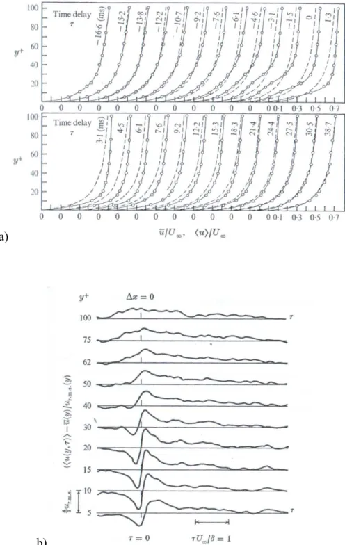
Blackwelder and Kaplan (1976), were among the first people to use the conditional sampling technique of Variable-Interval Time Averaging (VITA), to look at the structure of sweep events (see Bruun 1995). The VITA technique ensemble-averages signals based on a whether a turbulent event of rapidly changing quantity (e.g. velocity) is detected, such as a sweep or ejection passing through a probe. Using rakes of hotwires oriented in the wall-normal direction, Blackwelder and Kaplan (1976), were able to track a typical sweep event. The velocity profile during the sweep is plotted together with the

(34)

mean velocity profile in Fig. 2.2.3a. They observed that before the sweep was detected (-3.1ms < Ĳ < 0ms, Ĳ = 0 corresponds to the time of detection) there was an inflectional velocity profile, as also observed by Kline et al. (1967). After detection they observed a region of high speed fluid moving from the outer region and splashing onto the wall. Note also that after the burst has passed the instantaneous velocity profile was nearly identical to the time averaged profile (Ĳ > 30ms). Figure 2.2.3b shows the magnitude of the burst event throughout the boundary layer. Blackwelder and Kaplan (1976), observed that the signals were highly correlated in the wall normal direction, which suggested that the events affect a large region of the boundary layer. Their data also showed that the structures were skewed at an angle of around 20-30° to the streamwise direction.

In summary, the near wall region of a turbulent boundary layer is organized into streaks of low speed fluid, which are persistent and relatively quiescent for most of the time. The majority of the turbulent production in the entire boundary layer occurs in the buffer layer during violent, intermittent ‘ejections’ of low-speed fluid away from the wall and during inrushes of high-speed fluid towards the wall (‘sweeps’). This ‘bursting cycle’ is quasi-cyclic and self-generating. The recent Direct Numerical Simulation (DNS) study of Orlandi and Jimenez (1994) showed that it is the transport of high momentum fluid towards the wall (‘sweeps’) that is responsible for the high skin-friction in the turbulent boundary layer.

(35)

a)

b)

Figure 2.2.3. a) Conditionally averaged ‘burst’ event and mean velocity profiles at various time delays, Ĳ, relative to the point of detection (Ĳ = 0). b). Conditionally averaged hotwire signal at several wall normal locations. From Blackwelder and Kaplan (1976).

(36)

2.2.2. Outer Region

The outer region of the turbulent boundary layer is usually defined as the region y/į > 0.15, whereby the action of viscosity becomes less and less dominant (Panton, 2001). This region is not smooth, like the time averaged boundary layer profile, but consists of three-dimensional bulges that are of the same scale as the boundary layer thickness in both x and z. Deep irrotational valleys occur on the edges of these bulges, through which free-stream velocity is entrained into the turbulent region.

The outer layer exhibits a sharp interface between the turbulent interior and the non-turbulent exterior (Corrsin 1943, Corrsin and Kistler 1954). Conditional sampling techniques have been employed to study the intermittency and structure of the outer layer (Favre et al. 1965, and Kovasznay et al., 1970), which showed that these bulges are elongated in the streamwise direction. Flow visualisation studies by Falco (1977) showed ‘typical eddies’ or ‘Falco eddies’ on the upstream sides of the turbulent bulges, which moved towards the wall and are possibly responsible for the ‘sweep’ type motions near the wall (Fig. 2.2.4).

The debate is still open as to how the inner region interacts with the outer region and vice versa. There is, however, evidence of direct mass transfer through ‘ejections’ emanating from the wall (see Sec. 2.2.1). Also, indirect interactions occur through the growth of vortical structures from the wall to the outer regions. The effect of the outer boundary layer on the inner turbulent production process is not well understood. Panton (2001) stated that as the large outer flow eddy structure move along the wall, they impose pressure fluctuations on the inner region, hence influencing the near wall events.

(37)

Figure 2.2.4. The outer boundary layer structure showing a sharp interface between rotational turbulent flow within the boundary layer and irrotational free-stream flow. ‘Typical (Falco) eddies’ are formed on the back interfaces of the turbulent bulges. From Falco (1977).

(38)

2.2.3. Hairpin Vortices

The previous sections have shown that the turbulent boundary layer consists of a number of different types of coherent motions. Kline and Robinson (1989a and 1989b), attempted to organise coherent motions into classes. They tentatively proposed the following hierarchy of importance with respect to the creation of turbulent Reynolds stress and turbulent kinetic energy.

Most important and most active;

• Vortices – Vortex elements and vortical structures Play an important role;

• Ejections of low-speed fluid away from the wall

• Sweeps of high-speed fluid towards the wall

• Strong near wall shear layers Plays some role;

• Largeį-scale bulges in the outer region of the boundary layer

• Shear-layer “backs” of large-scale outer-region motions

• Near-wall “pockets”, visible in the laboratory as regions swept clear of marked near-wall fluid

• Low-speed streaks in the viscous sublayer.

Of the most important are vortical structures. It should be noted that any vortex element, except those located in the wall normal direction, has the potential to “pump” fluid away and towards the wall across the mean velocity gradient. It should therefore be of little surprise that vortex motions are so important in the production of turbulence kinetic energy.

(39)

In the early studies of the near wall structure and turbulence generation cycle, there was evidence to suggest that bursts and ejections may be part of structures that span the whole boundary layer region (Willmarth and Lu, 1972, and Lu and Willmarth, 1973, Blackwelder and Kaplan, 1976). Kovasznay (1970), postulated that there are a whole series of burst events of differing scales, whereby frequent small-scale bursts occur near the wall which grow or coalesce into large ones. This process was suggested to continue until the largest scale bursts reach the outer edge of the boundary layer, and are thus responsible for the ‘bulges’ (see Sherman (1990)). The existence of a dominant vortex structure throughout the whole boundary layer has received much attention over the years and investigations have been conducted into its form and regeneration mechanism.

Theodorsen (1952), proposed that turbulence is characterised by a definite three-dimensional flow pattern, and the motions it induces are responsible for the transfer of momentum and heat. Such structures were shown to be horseshoe or ring shaped in appearance, as depicted in Fig. 2.2.5, and were thought to cause almost all the dissipation in the turbulent boundary layer. This large-scale structure was proposed to be similar everywhere in wall-bounded turbulent flow and to have a different scale at different wall-normal distances.

(40)

Figure 2.2.5. Primary structure of wall-bound turbulence. From Theodorsen (1952).

Head and Bandyopadhyay (1981), were among the first to observe these hairpin structures in experiment and confirmed that nearly the entire boundary layer consisted of hairpin vortices, or stretched hairpin loops. It was certainly a surprise to them to see that something as complicated as the turbulent boundary layer had only one kind of dominant motion repeated over a range of scales. Using smoke flow visualisation and a laser sheet inclined to the wall, they were able to observe that the hairpin loops were straight over a large proportion of their length and were inclined, on average, at an angle of 45° to the wall into the flow. More recently using Particle Image Velocimetry (PIV), Liu et al. (1991) observed shear layers growing from the wall at 45° that ended with a region of spanwise vorticity - the heads of the hairpins. The cross-stream dimensions of the loops appeared to scale with the wall variables,

u* and Ȟ. However, the length of the hairpins appeared to be limited only by the boundary layer thickness, į. Thus the aspect ratio increased with the Reynolds number, as depicted in Fig. 2.2.6.

(41)

Robinson (1991a and 1991b), divided the hairpin structures into three parts; legs, neck and head as shown in Fig. 2.2.7. He emphasised that these are not necessarily symmetrical structures. In fact they are more common as asymmetric structures which are shaped like canes (also Moin and Kim, 1985). Robinson also suggested a link between the quasi-streamwise vortices and hairpin vortices (Fig. 2.2.8). Could it be that the counter-rotating legs of the hairpin vortices are actually responsible for the low speed streaks by the uplift of fluid between the legs? The topic is still subject to debate.

Figure 2.2.6. Effect of Reynolds number on hairpin structures in the outer boundary layer. a) Very low Re. b) Moderate Re. c) High Re. From Head and Bandyopadhyay (1981).

Figure 2.2.7. Parts of a horseshoe vortex as defined by Robinson (1991b).

U

(42)

Figure 2.2.8. Conceptual model of relationships between ejection/sweep and quasi-streamwise vortices in the near wall, and relationship between ejection/sweep and arch-shaped vortices in the outer region. From Robinson (1991b).

Figure 2.2.9. a) Schematic of a single hairpin vortex with the corresponding Q2 pumping in the neck region and the formation of a low-speed-streak between the legs. b) Signature of a hairpin in the x-y plane. From Adrian et al.

(43)

The characteristics of hairpins and their appearance in the x-y plane are presented in Fig. 2.2.9 according to Adrian et al., (2000). The vortex head was said to have a Q2 event (ejection) located beneath it and at around 45° to the wall, associated with the induced motion pumping fluid away from the wall due to the vortex neck. The legs of the vortex become quasi-streamwise near the wall with counter-rotation such that near-wall fluid between the legs is lifted away from the wall. There is also a stagnation zone marking the shear layer caused by the interaction of the Q2 event (ejection) with a Q4 event (sweep) above the structure. Using PIV, Adrian et al. (2000) observed that the hairpin structures were the single most readily observable flow pattern in a turbulent boundary layer from y+ § 50 right to the boundary layer edge. The angle that the neck and head make with the wall was observed to be a strong position of height, with the hairpins near the wall typically at 25-45° to it, and close to the boundary layer edge they are nearly vertical.

Head and Bandyopadhyay (1981), observed hairpin vortices to agglomerate into regular packets. Adrian et al. (2000), used PIV to show that these ‘packets’ often occur with more than 10 individual hairpins, all moving with a similar convection velocity so that they may be as long as 2įin the streamwise direction. In fact, they observed at least one hairpin vortex packet in 85% of their PIV images. It also appeared that many hairpin packets, each with their own convection velocity, seemed to coexist within other packets of different size and convection velocity. There appeared to be small, young packets lying close to the wall which exist within larger, older packets as depicted in Fig. 2.2.10.

(44)

Figure 2.2.10. Conceptual scenario of nested packets of hairpins or cane-type vortices growing up from the wall. These packets align in the streamwise direction and coherently add together to create large zones of nearly uniform streamwise momentum. Large-scale motions in the wake region ultimately limit their growth. Smaller packets move more slowly because they induce faster upstream propagation. Caption and Figure from Adrian et al. (2000).

(45)

The concept of hairpin ‘packets’ can account for much of the observed behaviour in a turbulent boundary layer. A single hairpin characteristically extends for a streamwise distance of x+ = 100 (Zhou et al. 1999), but low-speed-streaks often extend to x+ = 1000 (Kline et al. 1967). The occurrence of many sets of Q2 pumping from packets of hairpins would certainly enable low speed streaks to reach this length. The presence of many hairpins in a packet may also account for the meandering streaks since the hairpins will inherently have some spanwise variation in their individual locations. They also explain the multiple ejections observed by many authors, for example Corino and Brodkey (1969), whereby the passage of each individual hairpin in a packet produces its own Q2 event. The hairpin packet concept can also explain the oscillation observed before breakup in a ‘burst’ sequence. The oscillation may not be a temporal oscillation but a spatial oscillation caused by a series of Q2 events produced by each hairpin in the packet as it moves along the wall.

(46)

2.2.4. Turbulence Regeneration Cycle

The turbulent boundary layer is a self-sustaining phenomenon, such that new turbulence is constantly being created to counteract that dissipated as heat through viscous action. Many conceptual models have been produced to describe how the turbulence regenerates itself, based on the sweep-ejection cycle discussed in Sec. 2.2.1. These models can be categorised into parent-offspring or instability based mechanisms (Schoppa and Hussain 2002). Here, we shall focus only on selected parent-offspring mechanisms for brevity. Zhouet al. (1999), used DNS to study the development of a hairpin vortex and observed that a single hairpin does indeed have the ability to develop into a ‘hairpin packet’ provided it is sufficiently strong, as illustrated in Fig. 2.2.11. Thus, a hairpin vortex can naturally form a coherent packet, tent-like in appearance, with several hairpins upstream and downstream of the original hairpin. These self-sustaining properties make the hairpin vortex a fundamental flow structure in the turbulent boundary layer.

Choi (1989, 2001) presents a slightly different conceptual model to describe the self-generating turbulence events in the sweep-ejection cycle, as illustrated in Fig. 2.2.12. In the first stage of the model, a spanwise vortex filament is deformed by a near-wall burst event upstream of it. This causes the vortex to deform in the downstream direction, which is deformed further by the vortex filaments own self induction mechanism and due to the high shear near the wall (Stage 2). As the development proceeds further, hairpin vortices are created, and move away from the wall as an ejection motion. However, as neighbouring hairpin vortices ‘eject’, their legs come in close proximity and form a counter rotating pair with action so as to induce another sweep event,

(47)

which leads to high skin friction and provides the perturbation to the next (upstream) vortex filament. Thus the chain of turbulence producing events is complete and the sweep leads to an ejection which leads to a sweep and so on. More recently, Kim (2005), gives a summary of the self sustaining turbulence process in the turbulent boundary layer, as depicted in Fig. 2.2.13. He emphasises that a common feature of drag reducing flows, regardless of how drag was reduced, is near-wall streamwise vortices with reduced strength and increased spacing, thus indicating their importance in the turbulence generation process.

There is still much to learn about the turbulent boundary layer and the nature of turbulence itself. Although hairpin vortices seem dominant, there are many other vortex motions within the boundary layer which may also play key roles in the production of turbulence. With the rapid advancement in computational facilities and memory storage, DNS studies are becoming more and more complex and higher Reynolds number flows are now able to be solved (for example at ReĲ = 590 by Moser et al. 1999). It remains to be seen whether we

will ever fully understand the turbulent boundary layer and if and how the low-Reynolds number observations described above will translate to flight conditions (Andreopoulos et al. 1984).

(48)

Figure 2.2.11. The generation of a secondary hairpin vortex, SHV, upstream of the ȍ-shaped head of the primary hairpin vortex, PHV. Secondary vortex initiates from location marked A in b) and c). Also note formation of a downstream hairpin vortex, starting from streamwise vortices ahead of the head of the PHV. a) t+ = 63, b) t+ = 72, c) t+= 81, d) t+ = 117. From Zhou et al.(1999).

(49)

Figure 2.2.12. Conceptual model for the sequence of burst events from Choi (1989, 2001).

Figure 2.2.13. Schematic illustration of a self-sustaining process of near-wall turbulence structures. From Kim (2005).

(50)

2.3. Skin-Friction Drag Reduction

Through better understanding of the turbulent boundary layer, many strategies have been formulated to reduce skin-friction drag. The general approach is to provide some perturbation that will alter the sweep-ejection process described in Sec. 2.2. This has the aim of reducing the strength of the ‘sweep’ events, which are responsible for the majority of the skin-friction drag (Orlandi and Jiménez, 1994). The exact strategy and mechanism differs somewhat between techniques and there is much debate over the precise mechanism for a given technique. In this section we shall briefly review a few successful approaches of reducing skin-friction drag and move on to a detailed discussion of drag reduction by creating a spanwise oscillation at the wall. Overviews of drag reduction, including techniques for reducing pressure drag (i.e. streamlining) and postponing transition, can be found in Gad-el-Hak (2000), and Sellin and Moses (1989).

2.3.1. Overview

One of the most successful techniques of achieving skin-friction drag reduction is polymer or surfactant addition. These techniques involve adding tiny quantities of long chain polymers, or string-like surfactants, to liquids. Drag reductions of 70% have been achieved, which enables an increased flow rate or decreased pressure drop in turbulent pipe flow (Berman, 1978). In fact, polymer additives are used today in the Trans-Alaskan-Pipeline. The exact drag reduction mechanism has been discussed by Virk (1975), whereby the long chain-like molecules are believed to interfere with the turbulent bursting process by molecular extension. The additives appear to kill turbulence near

(51)

the wall, such that the laminar sublayer becomes thicker and the peak in turbulence intensity moves to higher y+.

Another successful technique, riblets, has been used on the hull of the Stars and Stripes, which won the Americas cup yacht race in 1987. Riblets are passive devices which consist of longitudinal grooves placed on the wall with depth, h, and spacing, s, of around the same order as the thickness as the viscous sublayer (h+ and s+ § 15 is optimal, Choi, 2001). Research on riblets began in the late 1970s by Walsh (see Walsh 1990). Many profiles of riblets have been studied and it is V-shaped grooves that are the most practical to manufacture. The concept seems to have been inspired by the skin of fast swimming sharks, which have rough dermal denticals with ridges that align with the flow direction. Drag reductions of around 8% have been observed using riblets, although their alignment must be within 30° of the mean flow direction in order to observe an effect. Choi (1987), deduced that the riblets act as small fences to restrict the movement of vortices near the wall. This weakens the induction velocity between adjacent quasi-streamwise vortices. Consequently, the near-wall bursts take place prematurely but at higher frequency which leads to a reduction in skin friction and turbulent intensity. The viscous sublayer also becomes thicker.

Another idea that has come from nature is the use of compliant coatings, which was inspired by dolphin’s skin (Kramer, 1961). Compliant coatings are deformable substances applied over a rigid wall. If the material properties are chosen such that the surface deformation is small and the material natural frequency,fo, is of the order of the average period between sweep events (50 < 1/fo+ < 150), then drag reductions of around 10% can be achieved (Choi et al.,