Publications
2016
Asynchronous Distributed ADMM for Large-Scale
Optimization—Part I: Algorithm and
Convergence Analysis
Tsung-Hui Chang
The Chinese University of Hong Kong
Mingyi Hong
Iowa State University, [email protected]
Wei-Cheng Liao
University of Minnesota - Twin Cities
Xiangfeng Wang
East China Normal University
Follow this and additional works at:
http://lib.dr.iastate.edu/imse_pubs
Part of the
Industrial Engineering Commons
,
Systems Architecture Commons
, and the
Systems
Engineering Commons
The complete bibliographic information for this item can be found at
http://lib.dr.iastate.edu/
imse_pubs/83
. For information on how to cite this item, please visit
http://lib.dr.iastate.edu/
howtocite.html
.
This Article is brought to you for free and open access by the Industrial and Manufacturing Systems Engineering at Iowa State University Digital Repository. It has been accepted for inclusion in Industrial and Manufacturing Systems Engineering Publications by an authorized administrator of Iowa State University Digital Repository. For more information, please [email protected].
arXiv:1509.02597v2 [cs.DC] 19 Feb 2016
Asynchronous Distributed ADMM for
Large-Scale Optimization- Part I:
Algorithm and Convergence Analysis
Tsung-Hui Chang⋆, Mingyi Hong†, Wei-Cheng Liao§ and Xiangfeng Wang‡
Abstract
Aiming at solving large-scale optimization problems, this paper studies distributed optimization methods based on the alternating direction method of multipliers (ADMM). By formulating the opti-mization problem as a consensus problem, the ADMM can be used to solve the consensus problem in a fully parallel fashion over a computer network with a star topology. However, traditional synchronized computation does not scale well with the problem size, as the speed of the algorithm is limited by the slowest workers. This is particularly true in a heterogeneous network where the computing nodes experience different computation and communication delays. In this paper, we propose an asynchronous distributed ADMM (AD-ADMM) which can effectively improve the time efficiency of distributed op-timization. Our main interest lies in analyzing the convergence conditions of the AD-ADMM, under the popular partially asynchronous model, which is defined based on a maximum tolerable delay of the network. Specifically, by considering general and possibly non-convex cost functions, we show that the AD-ADMM is guaranteed to converge to the set of Karush-Kuhn-Tucker (KKT) points as long as the algorithm parameters are chosen appropriately according to the network delay. We further illustrate that the asynchrony of the ADMM has to be handled with care, as slightly modifying the implementation of the AD-ADMM can jeopardize the algorithm convergence, even under the standard convex setting.
Keywords−Distributed optimization, ADMM, Asynchronous, Consensus optimization
Part of this work was submitted to IEEE ICASSP, Shanghai, China, March 20-25, 2016 [1]. Tsung-Hui Chang is supported by NSFC, China, Grant No. 61571385. Mingyi Hong is supported by NFS Grant No. CCF-1526078 , and AFOSR, Grant No. 15RT0767. Xiangfeng Wang is supported by Shanghai YangFan No. 15YF1403400 and NSFC No. 11501210.
⋆
Tsung-Hui Chang is the corresponding author. Address: School of Science and Engineering, The Chinese University of Hong Kong, Shenzhen, China 518172. E-mail: [email protected].
†
Mingyi Hong is with Department of Industrial and Manufacturing Systems Engineering, Iowa State University, Ames, 50011, USA, E-mail: [email protected]
†
Wei-Cheng Liao is with Department of Electrical and Computer Engineering, University of Minnesota, Minneapolis, MN 55455, USA, E-mail: [email protected]
‡
Xiangfeng Wang is with Shanghai Key Lab for Trustworthy Computing, School of Computer Science and Software Engineering, East China Normal University, Shanghai, 200062, China, E-mail: [email protected]
I. INTRODUCTION
A. Background
Scaling up optimization algorithms for future data-intensive applications calls for efficient distributed and parallel implementations, so that modern multi-core high performance computing technologies can be fully utilized [2]–[4]. In this work, we are interested in developing distributed optimization methods for solving the following optimization problem
min x∈Rn N X i=1 fi(x) +h(x), (1)
where eachfi :Rn→ Ris a (smooth) cost function;h:Rn→R∪ {∞} is a convex ( proper and lower
semi-continuous) but possibly non-smooth regularization function. The latter is used to impose desired structures on the solution (e.g., sparsity) and/or used to enforce certain constraints. Problem (1) includes as special cases many important statistical learning problems such as the LASSO problem [5], logistic regression (LR) problem [6], support vector machine (SVM) [7] and the sparse principal component analysis (PCA) problem [8]. In this paper, we focus on solving large-scale instances of these learning
problems with either a large number of training samples or a large number of features (n is large) [3].
These are typical data-intensive machine learning scenarios in which the data sets are often distributedly located in a few computing nodes. Traditional centralized optimization methods, therefore, fails to scale well due to their inability to handle distributed data sets and computing resources.
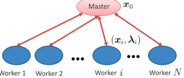
Our goal is to develop efficient distributed optimization algorithms over a computer network with a star topology, in which a master node coordinates the computation of a set of distributed workers (see Figure 1 for illustration). Such star topology represents a common architecture for distributed computing, therefore it has been used widely in distributed optimization [4], [9]–[16]. For example, under the star topology, references [10], [11] presented distributed stochastic gradient descent (SGD) methods, references [12], [13] parallelized the proximal gradient (PG) methods, while references [14]–[17] parallelized the block coordinate descent (BCD) method. In these works, the distributed workers iteratively calculate the gradients related to their local data, while the master collects such information from the workers to perform SGD, PG or BCD updates.
However, when scaling up these distributed algorithms, node synchronization becomes an important issue. Specifically, under the synchronous protocol, the master is triggered at each iteration only if it receives the required information from all the distributed workers. On the one hand, such synchronization is beneficial to make the algorithms well behaved; on the other hand, however, the speed of the algorithms
Master Master
Worker1 Worker2 Worker Worker
Fig. 1: A star computer cluster with one master and N workers.
would be limited by the “slowest” worker especially when the workers have different computation and communication delays. To address such dilemma, a few recent works [10]–[14] have introduced “asynchrony” into the distributed algorithms, which allows the master to perform updates when not all, but a small subset of workers have returned their gradient information. The asynchronous updates would cause “delayed” gradient information. A few algorithmic tricks such as delay-dependent step-size selection have been introduced to ensure that the staled gradient information does not destroy the stability of the algorithm. In practice, such asynchrony does make a big difference. As has been consistently reported in [10]–[14], under such an asynchronous protocol, the computation time can decrease almost linearly with the number of workers.
B. Related Works
A different approach for distributed and parallel optimization is based on the alternating direction method of multipliers (ADMM) [9, Section 7.1.1]. In the distributed ADMM, the original learning problem
is partitioned intoN subproblems, each containing a subset of training samples or the learning parameters.
At each iteration, the workers solve the subproblems and send the up-to-date variable information to the master, who summarizes this information and broadcasts the result to the workers. In this way, a given large-scale learning problem can be solved in a parallel and distributed fashion. Notably, other than the standard convex setting [9], the recent analysis in [18] has shown that such distributed ADMM is provably convergent to a Karush-Kuhn-Tucker (KKT) point even for non-convex problems.
Recently, the synchronous distributed ADMM [9], [18] has been extended to the asynchronous setting, similar to [10]–[14]. Specifically, reference [19] has considered a version of AD-ADMM with bounded delay assumption and studied its theoretical and numerical performances. However, only convex cases are considered in [19]. Reference [20] has studied another version of AD-ADMM for non-convex problems, which considers inexact subproblem updates and, similar to [10]–[14], the workers compute gradient
computation powers of distributed nodes. Besides, due to inexact update, such schemes usually require more iterations to converge and thus may have higher communication overhead. References [21]–[23] have respectively considered asynchronous ADMM methods for decentralized optimization over networks. These works consider network topologies beyond the star network, but their definition of asynchrony is different from what we propose here. Specifically, the asynchrony in [21] lies in that, at each iteration, the nodes are randomly activated to perform variable update. The method presented in [22] further allows that the communications between nodes can succeed or fail randomly. It is shown in [22] that such asynchronous ADMM can converge in a probability-one sense, provided that the nodes and communication links satisfy certain statistical assumption. Reference [23] has considered an asynchronous dual ADMM method. The asynchrony is in the sense that the nodes are partitioned into groups based on certain coloring scheme and only one group of nodes update variable in each iteration.
C. Contributions
In this paper1, we generalize the state-of-the-art synchronous distributed ADMM [9], [18] to the
asynchronous setting. Like [10]–[14], [19], [20], the asynchronous distributed ADMM (AD-ADMM) algorithm developed in this paper gives the master the freedom of making updates only based on variable information from a partial set of workers, which further improves the computation efficiency of the distributed ADMM.
Theoretically, we show that, for general and possibly non-convex problems in the form of (1), the AD-ADMM converges to the set of KKT points if the algorithm parameters are chosen appropriately according to the maximum network delay. Our results differ significantly from the existing works [19], [21], [22] which are all developed for convex problems. Therefore, the analysis and algorithm proposed here are applicable not only to standard convex learning problems but also to important non-convex problems such as the sparse PCA problem [8] and matrix factorization problems [24]. To the best of our knowledge, except the inexact version in [20], this is the first time that the distributed ADMM is rigorously shown to be convergent for non-convex problems under the asynchronous protocol. Moreover, unlike [19], [21], [22] where the convergence analyses all rely on certain statistical assumption on the nodes/workers, our convergence analysis is deterministic and characterizes the worst-case convergence conditions of the AD-ADMM under a bounded delay assumption only. Furthermore, we demonstrate that the asynchrony of ADMM has to be handled with care – as a slight modification of the algorithm may
1
lead to completely different convergence conditions and even destroy the convergence of ADMM for convex problems. Some numerical results are presented to support our theoretical claims.
In the companion paper [25], the linear convergence conditions of the AD-ADMM is further analyzed. In addition, the numerical performance of the AD-ADMM is examined by solving a large-scale LR problem on a high-performance computer cluster.
Synopsis: Section II presents the applications of problem (1) and reviews the distributed ADMM in
[9]. The proposed AD-ADMM and its convergence conditions are presented in Section III. Comparison of the proposed AD-ADMM with an alternative scheme is presented in Section IV. Some simulation results are presented in Section V. Finally, concluding remarks are given in Section VI.
II. APPLICATIONS ANDDISTRIBUTEDADMM
A. Applications
We target at solving problem (1) over a star computer network (cluster) with one master node and N
workers/slaves, as illustrated in Figure 1. Such distributed optimization approach is extremely useful in modern big data applications [3]. For example, let us consider the following regularized empirical risk minimization problem [7] min w∈Rn m X j=1 ℓ(aTjw, yj) + Ω(w), (2)
where m is the number of training samples and ℓ(aTjw, yj) is a loss function (e.g., regression or
classification error) that depends on the training sample aj ∈ Rn, label yj and the parameter vector
w ∈ Rn. Here, n denotes the dimension of the parameters (features); Ω(w) is an appropriate convex
regularizer. Problem (2) is one of the most important problems in signal processing and statistical learning, which includes the LASSO problem [26], LR [6], SVM [7] and the sparse PCA problem [8], to name a few. Obviously, solving (2) can be challenging when the number of training samples is very large. In that case, it is natural to split the training samples across the computer cluster and resort to a distributed
optimization approach. Suppose that themtraining samples are uniformly distributed and stored by theN
workers, with each nodeigettingqi=xm/Ny samples. By definingfi(w),Piqj=(i i−1)qi+1ℓ(aTjw, yj),
i= 1, . . . , N, andh(w),Ω(w), it is clear that (2) is an instance of (1).
When the number of training samples is moderate but the dimension of the parameters is very large
(n ≫ m), problem (2) is also challenging to solve. By [9, Section 7.3], one can instead consider the
Lagrangian dual problem of (2) provided that (2) has zero duality gap. Specifically, let the training
matrix A ,[a1, . . . ,am]T ∈Rm×n be partitioned as A= [A
wbe partitioned conformally asw= [wT
1, . . . ,wTN]T; moreover, assume thatΩ is separable asΩ(w) = PN
i=1Ωi(wi). Then, following [9, Section 7.3], one can obtain the dual problem of (2) as
min ν∈Rm N X i=1 Ω∗i(ATi ν) + Φ∗(ν), (3)
where ν , [ν1, . . . , νm]T is a dual variable, Φ∗(ν) = Pm
j=1ℓ∗(νj, yj), and ℓ∗ and Ω∗i are respectively
the conjugate functions of ℓand Ωi. Note that (3) is equivalent to splitting the n parameters across the
N workers. Clearly, problem (3) is an instance of (1).
It is interesting to mention that many emerging problems in smart power grid can also be formulated as problem (1); see, for example, the power state estimation problem considered in [27] is solved by employing the distributed ADMM. The energy management problems (i.e., demand response) in [28]–[30] can potentially be handled by the distributed ADMM as well.
B. Distributed ADMM
In this section, we present the distributed ADMM [4], [9] for solving problem (1). Let us consider the following consensus formulation of problem (1)
min x0,xi∈Rn, i=1,...,N N X i=1 fi(xi) +h(x0) (4a) s.t. xi=x0, ∀i= 1, . . . , N. (4b)
In (4), the N + 1 variables xi, i = 0,1, . . . , N, are subject to the consensus constraint in (4b), i.e.,
x0=x1=· · ·=xN. Thus, problem (4) is equivalent to (1).
It has been shown that such a consensus problem can be efficiently solved by the ADMM [9]. To
describe this method, let λ∈Rn denote the Lagrange dual variable associated with constraint (4b) and
define the following augmented Lagrangian function Lρ(x,x0,λ) = N X i=1 fi(xi) +h(x0) + N X i=1 λTi (xi−x0) +ρ 2 N X i=1 kxi−x0k2, (5) where x,[xT
1, . . . ,xTN]T, λ,[λT1, . . . ,λTN]T andρ >0 is a penalty parameter. According to [4], the
standard synchronous ADMM iteratively updates the primal variablesxi, i= 0,1, . . . , N, by minimizing
(5) in a (one-round) Gauss-Seidel fashion, followed by updating the dual variableλusing an approximate
Algorithm 1 (Synchronous) Distributed ADMM for (4) [9] 1: Given initial variablesx0 andλ0; set x0
0=x0 and k= 0. 2: repeat 3: update xk+1 0 = arg min x0∈Rn h(x0)−xT 0 PN i=1λki +ρ2PNi=1kxk i −x0k2 , (6) xk+1 i = arg min xi∈Rn fi(xi) +xTi λki + ρ 2kxi−x k+1 0 k2, ∀i= 1, . . . , N, (7) λk+1 i =λ k i +ρ(xki+1−x k+1 0 ), ∀i= 1, . . . , N. (8) 4: set k←k+ 1.
5: until a predefined stopping criterion is satisfied.
As seen, Algorithm 1 is naturally implementable over the star computer network illustrated in Figure
1. Specifically, the master node takes charge of optimizing x0 by (6), and each worker iis responsible
for optimizing (xi,λi) by (7)-(8). Through exchanging the up-to-date x0 and (xi,λi) between the
master and the workers, Algorithm 1 solves problem (1) in a fully distributed and parallel manner. Convergence properties of the distributed ADMM have been extensively studied; see, e.g., [9], [18], [31]–[33]. Specifically, [31] shows that the ADMM, under general convex assumptions, has a worst-case
O(1/k) convergence rate; while [32] shows that the ADMM can have a linear convergence rate given
strong convexity and smoothness conditions on fi’s. For non-convex and smooth fi’s, the work [18]
shows that Algorithm 1 can converge to the set of KKT points with aO(1/√k)rate as long asρ is large
enough.
However, Algorithm 1 is a synchronous algorithm, where the operations of the master and the workers
are “locked” with each other. Specifically, to optimize x0 at each iteration, the master has to wait until
have different computation and communication delays2, the pace of the optimization would be determined
by the “slowest” worker. As an example illustrated in Figure 2(a), the master updatesx0 only when it
has received the variable information for the four workers at every iteration. As a result, under such synchronous protocol, the master and speedy workers (e.g., workers 1 and 3 in Figure 2) would spend most of the time idling, and thus the parallel computational resources cannot be fully utilized.
III. ASYNCHRONOUSDISTRIBUTED ADMM
A. Algorithm Description
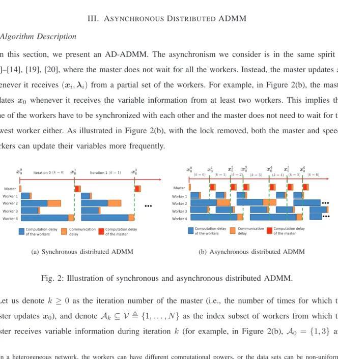
In this section, we present an AD-ADMM. The asynchronism we consider is in the same spirit of
[10]–[14], [19], [20], where the master does not wait for all the workers. Instead, the master updatesx0
whenever it receives(xi,λi) from a partial set of the workers. For example, in Figure 2(b), the master
updates x0 whenever it receives the variable information from at least two workers. This implies that
none of the workers have to be synchronized with each other and the master does not need to wait for the slowest worker either. As illustrated in Figure 2(b), with the lock removed, both the master and speedy workers can update their variables more frequently.
Iteration0 Iteration1 Worker1 Master Worker2 Worker3 Worker4
Computationdelay Communication Computationdelay oftheworkers delay ofthemaster
(a) Synchronous distributed ADMM
Worker1 Master
Worker2 Worker3 Worker4
Computation delay Communication Computation delay Computationdelay oftheworkers Communication delay Computationdelay ofthemaster
(b) Asynchronous distributed ADMM
Fig. 2: Illustration of synchronous and asynchronous distributed ADMM.
Let us denote k ≥0 as the iteration number of the master (i.e., the number of times for which the
master updates x0), and denote Ak ⊆ V ,{1, . . . , N} as the index subset of workers from which the
master receives variable information during iteration k (for example, in Figure 2(b), A0 = {1,3} and
2
In a heterogeneous network, the workers can have different computational powers, or the data sets can be non-uniformly distributed across the network. Thus, the workers can require different computational times in solving the local subproblems. Besides, the communication delays can also be different, e.g., due to probabilistic communication failures and message retransmission.
A1 = {1,2})3. We say that worker i is “arrived” at iteration k if i ∈ Ak and “unarrived” otherwise.
Clearly, unbounded delay will jeopardize the algorithm convergence. Therefore throughout this paper, we will assume that the asynchronous delay in the network is bounded. In particular, we follow the popular partially asynchronous model [4] and assume:
Assumption 1 (Bounded delay) Let τ ≥1 be a maximum tolerable delay. For all i∈ V and iteration
k≥0, it must be thati∈ Ak∪ Ak−1· · · ∪ Amax{k−τ+1,−1}.
Assumption 1 implies that every worker i is arrived at least once within the period [k−τ + 1, k].
In another word, the variable information (xi,λi) used by the master must be at most τ iterations old.
To guarantee the bounded delay, at every iteration the master should wait for the workers who have
been inactive for τ−1 iterations, if such workers exist. Note that, when τ = 1, one hasi∈ Ak for all
i∈ V (i.e.,Ak =V), which corresponds to the synchronous case and the master always waits for all the
workers at every iteration.
In Algorithm 2, we present the proposed AD-ADMM, which specifies respectively the steps for the
master and the distributed workers. Here, Ac
k denotes the complementary set of Ak, i.e.,Ak∩ Ack =∅
and Ak ∪ Ack = V. Algorithm 2 has five notable differences compared with Algorithm 1. First, the
master is required to update {(xi,λi)}i∈V, and such update is only performed for those variables with
i ∈ Ak. Second, x0 is updated by solving a problem with an additional proximal term γ2kx0−xk0k2,
where γ > 0 is a penalty parameter (cf. (12)). Adding such proximal term is crucial in making the
algorithm well-behaved in the asynchronous setting. As will be seen in the next section, a proper choice
of γ guarantees the convergence of Algorithm 2. Third, the variables di’s are introduced to count the
delays of the workers. If worker iis arrived at the current iteration, then di is set to zero; otherwise, di
is increased by one. So, to ensure Assumption 1 hold all the time, in Step 4 of Algorithm of the Master,
the master waits if there exists at least one worker whosedi≥τ−1. Fourth, in addition to the bounded
delay, we assume that the master proceeds to update the variables only if there are at leastA≥1arrived
workers, i.e., |Ak| ≥A for allk [19]. Note that whenA=N, the algorithm reduces to the synchronous
distributed ADMM. Fifth, in Step 6 of Algorithm of the Master, the master sends the up-to-date x0 only
to the arrived workers.
We emphasize again that both the master and fast workers in the AD-ADMM can have less idle time and update more frequently than its synchronous counterpart. As illustrated in Figure 2, during the
3Without loss of generality, we letA
same period of time, the synchronous algorithm only completes two updates whereas the asynchronous algorithm updates six times already. On the flip side, the asynchronous algorithm introduces delayed variable information and thereby requires a larger number of iterations to reach the same solution accuracy than its synchronous counterpart. In practice we observe that the benefit of improved update frequency can outweigh the cost of increased number of iterations, and as a result the asynchronous algorithm can still converge faster in time. This is particularly true when the workers have different computation and communication delays and when the computation and communication delays of the master for solving (12) is much shorter than the computation and communication delays of the workers for updating (13)
and (14)4; e.g., see Figure 2. Detailed numerical results will be reported in Section V of the companion
paper [25].
B. Convergence Analysis
In this subsection, we analyze the convergence conditions of Algorithm 2. We first make the following standard assumption on problem (1) (or equivalently problem (4)):
Assumption 2 Each function fi is twice differentiable and its gradient∇fi is Lipschitz continuous with
a Lipschitz constantL >0; the functionh is proper convex (lower semi-continuous, but not necessarily smooth) and dom(h) (the domain ofh) is compact. Moreover, problem (1) is bounded below, i.e., F⋆>
−∞ whereF⋆ denotes the optimal objective value of problem (1).
Notably, we do not assume any convexity onfi’s. Indeed, we will show that the AD-ADMM can converge
to the set of KKT points even for non-convex fi’s. Our main result is formally stated below.
Theorem 1 Suppose that Assumption 1 and Assumption 2 hold true. Moreover, assume that there exists
a constantS ∈[1, N] such that |Ak|< S for all k and that
∞>Lρ(x0,x00,λ0)−F⋆ ≥0, (15) ρ > (1 +L+L 2) +p(1 +L+L2)2+ 8L2 2 , (16) γ > S(1 +ρ 2)(τ −1)2−N ρ 2 . (17) 4
Note that, for many practical cases (such ash(x0) =kx0k1) for which (12) has a closed-form solution, the computation delay
of the master is negligible. For high-performance computer clusters connected by large-bandwidth fiber links, the communication delays between the master and the workers can also be short. However, for cases in which the computation and communication delays of the master is significant, the AD-ADMM could be less time efficient than the synchronous ADMM due to the increased number of iterations.
Then, ({xk
i}Ni=1,xk0,{λki}Ni=1) generated by (9), (10) and (12) are bounded and have limit points which
satisfy KKT conditions of problem (4).
Theorem 1 implies that the AD-ADMM is guaranteed to converge to the set of KKT points as long as
the penalty parameters ρ and γ are sufficiently large. Since 1/γ can be viewed as the step size of x0,
(17) indicates that the master should be more cautious in movingx0 if the network allows a longer delay
τ. In particular, the value γ in the worst case should increase with the order of τ2. When τ = 1 (the
synchronous case), γ =−(N ρ)/2 <0 and thus the proximal term γ2kx0−xk
0k2 can be removed from
(12). On the other hand, we also see from (17) thatγ should increase with N if τ >1 is fixed5. This is
because in the worst case the more workers, the more outdated information introduced in the network.
Finally, we should mention that a large ρ may be essential for the AD-ADMM to converge properly,
especially for non-convex problems, as we demonstrate via simulations in Section V.
Let us compare Theorem 1 with the results in [19], [22]. First, the convergence conditions in [19], [22] are only applicable for convex problems, whereas our results hold for both convex and non-convex problems. Second, [19], [22] have made specific statistical assumptions on the behavior of the workers, and the convergence results presented therein are in an expectation sense. Therefore it is possible, at least theoretically, that a realization of the algorithm fails to converge despite satisfying the conditions given in [19]. On the contrary, our convergence results hold deterministically.
Note that for non-convex fi’s, subproblem (13) is not necessarily convex. However, given ρ ≥ L
in (16) and twice differentiability of fi (Assumption 2), subproblem (13) becomes a (strongly) convex
problem6 and hence is globally solvable. When fi’s are all convex functions, Theorem 1 reduces to the
following corollary.
Corollary 1 Assume that fi’s are all convex functions. Under the same premises of Theorem 1, and for
γ satisfying (17) and
ρ≥ (1 +L
2) +p(1 +L2)2+ 8L2
2 , (18)
({xki}Ni
=1,xk0,{λki}Ni=1)generated by (9), (10) and (12) are bounded and have limit points which satisfy
KKT conditions of problem (4).
5Note that, for a fixedτ,S should increase withN.
6By [34, Lemma 1.2.2], the minimum eigenvalue of the Hessian matrix off
i(xi)is no smaller than−L. Thus, forρ > L, subproblem (13) is a strongly convex problem.
C. Proof of Theorem 1 and Corollary 1
Let us write Algorithm 2 from the master’s point of view. Definek¯i as the last iteration number before
iterationk for which workeri∈ Ak is arrived7, i.e.,i∈ A¯ki. Then Algorithm 2 from the master’s point
of view is as follows: for master iteration k= 0,1, . . . ,
xk+1 i = arg min xi fi(xi) +xTi λ ¯ ki+1 i + ρ2kxi−x¯ki+1 0 k2 , ∀i∈ Ak xk i ∀i∈ Ack , (19) λk+1 i = λk¯i+1 i +ρ(x k+1 i −x ¯ ki+1 0 ) ∀i∈ Ak λk i ∀i∈ Ack , (20) xk+1 0 = arg min x0∈Rn h(x0)−xT 0 PN i=1λki+1 +ρ2PNi=1kxk+1 i −x0k2+ γ 2kx0−xk0k2 .
Now it is relatively easy to see that the master updates x0 using the delayed (xi,λi)i∈A
k and the old
(xi,λi)i∈Ac
k. Under Assumption 1, it must hold
max{k−τ,−1} ≤k¯i< k ∀k≥0. (21)
Moreover, by the definition of ¯ki it holds that i /∈ Ak−1∪ · · · ∪ A¯ki+1, therefore we have that
λ¯ki+1 i =λ ¯ ki+2 i =· · ·=λ k i, ∀i∈ Ak. (22)
By applying (22) to (19) and (20) (replacing λ¯ki+1
i with λki), we rewrite the master-point-of-view
algorithm in Algorithm 3.
Inspired by [18], our analysis for Theorem 1 investigates how the augmented Lagrangian function, i.e., Lρ(xk,xk0,λk) = N X i=1 fi(xki) +h(xk0) + N X i=1 (λki)T(xki −xk 0) +ρ 2 N X i=1 kxki −xk 0k2 (26)
evolves with the iteration numberk, where xk,[(xk
1)T, . . . ,(xkN)T]T and λk,[(λk1)T, . . . ,(λkN)T]T.
The following lemma is one of the keys to prove Theorem 1.
7Note thatk¯
Lemma 1 Suppose that Assumption 2 holds and ρ≥L. Then, it holds that Lρ(xk+1,xk0+1,λk+1)− Lρ(xk,xk0,λk) ≤ −2γ+N ρ 2 kx k+1 0 −xk0k2 + 1 ρ + 1 2 X i∈Ak kλk+1 i −λ k ik2 +1 +ρ 2 2 X i∈Ak kxk¯i+1 0 −xk0k2 +(1−ρ) +L 2 X i∈Ak kxk+1 i −x k ik2. (27)
Proof: See Appendix A.
Equation (27) shows thatLρ(xk,xk0,λk)is not necessarily decreasing due to the error terms
P i∈Akk λk+1 i − λk ik2 and P i∈Akk x¯ki+1
0 −xk0k2. Next we bound the sizes of these two terms.
First considerPi∈Akkλk+1
i −λkik2. Note from (24) and the optimality condition of (23) that,∀i∈ Ak,
0=∇fi(xk+1 i ) +λ k i +ρ(xki+1−x ¯ ki+1 0 ) =∇fi(xki+1) +λ k+1 i . (28) For anyi∈ Ac
k, denoteeki < k as the last iteration number for which workeri is arrived. Then,i∈ Aeki
and thus ∇fi(x e ki+1 i ) +λ e ki+1 i = 0. Since x e ki+1 i = x e ki+2 i = · · · =xki = x k+1 i and λ e ki+1 i = λ e ki+2 i = · · ·=λk i =λ k+1 i , we obtain that ∇fi(xki+1) +λ k+1
i =0∀i∈ Ack. Therefore, we conclude that
∇fi(xki+1) +λ k+1
i =0, ∀ i∈ V and ∀ k. (29)
By (29) and the Lipschitz continuity of ∇fi (Assumption 2), we can bound
kλk+1 i −λkik2 ≤ k∇fi(xik+1)− ∇fi(xki)k2 ≤L2kxk+1 i −x k ik2, ∀ i∈ V. (30)
By applying (30), we can further write (27) as Lρ(xk+1,xk0+1,λk+1) ≤ Lρ(xk,xk0,λk) + 1 +ρ2 2 X i∈Ak kxk 0−x ¯ ki+1 0 k2 − 2γ+N ρ 2 kxk+1 0 −xk0k2 + L+L2+ (1−ρ) 2 + L2 ρ X i∈Ak kxk+1 i −xkik2. (31)
From (31), one can observe that the error term (1+2ρ2)Pi∈Akkxk
0 −x
¯
ki+1
0 k2 is present due to the
asynchrony of the network. The next lemma bounds this error term:
Lemma 2 Suppose that Assumption 1 holds and assume that |Ak| < S for all k, for some constant
S∈[1, N]. Then, it holds that
k X j=0 X i∈Aj kxj 0−x ¯ ji+1 0 k2 ≤S(τ −1)2 k−1 X j=0 kxj+1 0 −x j 0k2. (32)
Proof: See Appendix B.
The last lemma shows that Lρ(xk,xk0,λk) is bounded below:
Lemma 3 Under Assumption 2 and for ρ≥L, it holds that
Lρ(xk+1,xk0+1,λk+1)≥F⋆ >−∞. (33)
Proof: See Appendix C.
Given the three lemmas above, we are ready to prove Theorem 1.
Proof of Theorem 1: Note that any KKT point ({x⋆
i}Ni=1,x⋆0,{λ⋆i}Ni=1) of problem (4) satisfies the following conditions ∇fi(x⋆i) +λ⋆i =0, ∀ i∈ V, (34a) s⋆ 0−PNi=1λ⋆i =0, (34b) x⋆i =x⋆ 0, ∀ i∈ V, (34c) where s⋆
0 ∈∂h(x⋆0)denotes a subgradient ofh atx⋆0 and∂h(x⋆0) is the subdifferential ofh atx⋆0. Since (34) also implies N X i=1 ∇fi(x⋆)+s⋆0 =0, (35) where x⋆,x⋆
To prove the desired result, we take a telescoping sum of (31), which yields Lρ(xk+1,xk0+1,λk+1)− Lρ(x0,x00,λ0) ≤ 1 +ρ2 2 Xk j=0 X i∈Aj kxj 0−x ¯ ji+1 0 k2 + L+L2+ (1−ρ) 2 + L2 ρ Xk j=0 X i∈Aj kxj+1 i −x j ik2 − 2γ+N ρ 2 Xk j=0 kxj+1 0 −x j 0k2. (36)
By substituting (32) in Lemma 2 into (36), we obtain
2γ+N ρ−S(1 +ρ2)(τ −1)2 2 Xk−1 j=0 kxj+1 0 −x j 0k2 + (1−ρ)−(L+L2) 2 − L2 ρ Xk j=0 N X i=1 kxj+1 i −x j ik2 ≤ Lρ(x0,x00,λ0)− Lρ(xk+1,xk0+1,λk+1) = (Lρ(x0,x00,λ0)−F⋆)−(Lρ(xk+1,x0k+1,λk+1)−F⋆) ≤ Lρ(x0,x00,λ0)−F⋆<∞, (37)
where the second inequality is obtained by applying Lemma 3, and the last strict inequality is due to
Assumption 2 where the optimal value F⋆ is assumed to be lower bounded.
Then, (16) and (17) imply that the left hand side (LHS) of (37) is positive and increasing with k. Since
the RHS of (37) is finite, we must have, as k→ ∞,
xk+1 0 −xk0 →0, xki+1−x k i →0, ∀ i∈ V. (38) Given (30), (38) infers λk+1 i −λ k i →0, ∀i∈ V. (39)
We use (38) and (39) to show that every limit point of ({xk
i}Ni=1,xk0,{λki}Ni=1) is a KKT point of
problem (4). Firstly, by applying (39) to (24) and by (38), one obtains xk+1
0 −xki+1 →0 ∀i∈ Ak. For
i∈ Ac
k, note that i∈ Aeki (see the definition of eki above (29)) and thus, by (24),
λeki+1 i =λ e ki i +ρ(x e ki+1 i −x (eki)i+1 0 ),
where(eki)i denotes the last iteration number before iterationeki for which workeriis arrived. Moreover,
since xeki+1
i =x
e ki+2
i =· · ·=xki =xki+1 ∀i∈ Ack, and by (24), (38) and (39), we have∀i∈ Ack,
kxk+1 0 −xki+1k=kx k+1 0 −x e ki+1 i k =kxk+1 0 −x (eki)i+1 0 +x (eki)i+1 0 −x e ki+1 i k ≤ kxk+1 0 −x (eki)i+1 0 k+ 1 ρkλ e ki+1 i −λ e ki i k →0. (40) So we conclude xk+1 0 −xki+1 →0 ∀i∈ V. (41)
Secondly, the optimality condition of (25) gives
sk+1 0 − N X i=1 λk+1 i −ρ N X i=1 (xk+1 i −x k+1 0 ) +γ(xk+1 0 −xk0) =0, (42) for somesk+1
0 ∈∂h(xk0+1). By applying (41) and (38) to (42), we obtain that
sk+1 0 − N X i=1 λk+1 i →0. (43)
Equations (29), (41) and (43) imply that ({xk
i}Ni=1,xk0,{λki}Ni=1) asymptotically satisfy the KKT condi-tions in (34).
Lastly, let us show that ({xki}Ni
=1,xk0,{λki}Ni=1) is bounded and has limit points. Since dom(h) is
compact and xk
0 ∈ dom(h), x0k is a bounded sequence and thus has limit points. From (41), xki,i∈ V,
are bounded and have limit points. Moreover, by (29), λki, i∈ V, are bounded and have limit points as
well. In summary, ({xki}Ni
=1,xk0,{λki}Ni=1) converges to the set of KKT points of problem (4) .
Proof of Corollary 1: The proof exactly follows that of Theorem 1. The only difference is that the
coefficient of the term (1−ρ2)+LPi∈Akkxk+1
i −xkik2 in (27) reduces from (1−ρ)+L 2 to (1−ρ) 2 ; see the footnote in Appendix A.
IV. COMPARISON WITH ANALTERNATIVESCHEME
In Algorithm 2, the workers compute (xi,λi), i ∈ V, and the master is in charge of computing
other valid implementations, and if so, how they compare with Algorithm 2. To shed some light on this question, we consider in this section an alternative scheme in Algorithm 4.
Algorithm 4 differs from Algorithm 2 in that the master handles not only the update ofx0 but also that
of {λi}i∈V; so the workers only updates{xi}. In essence, in a synchronous network, Algorithm 2 and
Algorithm 4 are equivalent up to a change of update order8 and have the same convergence conditions.
However, intriguingly, in an asynchronous network, the two algorithms may require distinct convergence conditions and behave very differently in practice. To analyze the convergence of Algorithm 4, we make the following assumption.
Assumption 3 Each function fi is strongly convex with modulus σ2>0 and the function h is convex.
Under the strong convexity assumption, we are able to show the following convergence result for Algorithm 4.
Theorem 2 Suppose that Assumption 1 and Assumption 3 hold true. Moreover, let γ = 0 and 0< ρ≤ σ 2 (5τ−3) max{2τ,3(τ −1)}, (48) and define x¯k i = 1k Pk
ℓ=1xki ∀i = 0,1, . . . , N, where ({xki}Ni=1,xk0) are generated by (44) and (45).
Then, it holds that
XN i=1 fi( ¯xki) +h( ¯xk0) −F⋆ + N X i=1 kx¯ki −x¯k 0k ≤ (2 +δλ)C k (49)
for allk, where C <∞ is a finite constant and δλ ,max{kλ⋆1k, . . . ,kλ⋆Nk}, in which{λ⋆i} denote the
optimal dual variables of (4).
The proof is presented in Appendix D. Theorem 2 somehow implies that Algorithm 4 may require
stronger convergence conditions than Algorithm 2 in the asynchronous network, as fi’s are assumed to
be strongly convex. Besides, different from Theorem 1 where ρ is advised to be large for Algorithm 2,
Theorem 2 indicates thatρneeds to be small for Algorithm 4. Sinceρ is the step size of the dual gradient
ascent in (46), (48) implies that the master should move λi’s slowly when τ is large. Such insight is
reminiscent of the recent convergence results for multi-block ADMM in [33].
Interestingly and surprisingly, our numerical results to be presented shortly suggest that the strongly
convexfi’s and a small ρ are necessary for the convergence of Algorithm 4.
8
V. SIMULATION RESULTS
The main purpose of this section is to examine the convergence behavior of the AD-ADMM with
respect to the master’s iteration number k. So, the simulation results to be presented are obtained by
implementing Algorithm 3 on a desktop computer. First, we present the simulation results of the AD-ADMM for solving the non-convex sparse PCA problem. Second, we consider the LASSO problem and compare Algorithm 4 with Algorithm 2.
A. Example 1: Sparse PCA
Theorem 1 has shown that the AD-ADMM can converge for non-convex problems. To verify this point, let us consider the following sparse PCA problem [8]
min w∈Rn − N X j=1 wTBTj Bjw+θkwk1, (50)
where Bj ∈Rm×n, ∀j = 1, . . . , N, andθ > 0 is a regularization parameter. The sparse PCA problem
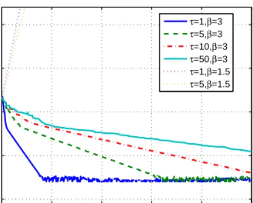
above is not a convex problem. We display in Figure 3 the convergence performance of the AD-ADMM
for solving (50). In the simulations, each matrix Bj ∈Rn is a 1000×500 sparse random matrix with
approximately 5000 non-zero entries; θ is set to 0.1 and N = 32. The penalty parameter ρ is set to
ρ = βmaxj=1,...,Nλmax(BjTBj) and γ = 0. To simulate an asynchronous scenario, at each iteration,
half of the workers are assumed to have a probability 0.1 to be arrived independently, and half of the workers are assumed to have a probability 0.8 to be “arrived” independently. At each iteration, the master
proceeds to update the variables as long as there is at least one arrived worker, i.e.,A= 1. The accuracy
is defined as accuracy = |Lρ(x k,xk 0,λk)−Fˆ| ˆ F (51)
where Fˆ denotes the optimal objective value for the synchronous case (τ = 1) which is obtained by
running the distributed ADMM (withβ = 3) for 10000 iterations (it is found in the experiments that the
AD-ADMM converges to the same KKT point for different values ofτ). One can observe from Figure 3
that the AD-ADMM (withβ = 3) indeed converges properly even though (50) is a non-convex problem.
Interestingly, we note that for the example considered here, the AD-ADMM withγ = 0works well for
different values of τ, even though Theorem 1 suggests thatγ should be a larger value in the worst-case.
However, we do observe from Figure 3 that if one sets β = 1.5 (i.e., a smaller value of ρ), then the
AD-ADMM diverges even in the synchronous case (τ = 1). This implies that the claim of a large enough
0 100 200 300 400 500 10−20 10−10 100 1010 1020 Iteration Accuracy τ=1,β=3 τ=5,β=3 τ=10,β=3 τ=50,β=3 τ=1,β=1.5 τ=5,β=1.5
Fig. 3: Convergence curves of the AD-ADMM (Algorithm 2) for solving the sparse PCA problem (50);
N = 32, θ= 0.1, ρ=βmaxj=1,...,Nλmax(BjTBj) andγ = 0.
B. Example 2: LASSO
In this example, we compare the convergence performance of Algorithm 4 with Algorithm 2. We consider the following LASSO problem
min w∈Rn N X i=1 kAiw−bik2+θkwk1, (52) where Ai ∈ Rm×n, b
i ∈Rm, i = 1, . . . , N, and θ > 0. The elements of Ai’s are randomly generated
following the Gaussian distribution with zero mean and unit variance, i.e.,∼ N(0,1); eachbi is generated
bybi=Aiw0+νi wherew0 ∈Rnis ann×1sparse random vector with approximately0.05nnon-zero
entries and νi is a noise vector with entries following N(0,0.01). A star network with 16 (N = 16)
workers is considered. To simulate an asynchronous scenario, at each iteration, half of the workers are assumed to have a probability 0.1 to be arrived independently, 4 workers are assumed to have a probability 0.3 to be arrived independently, and the remaining 4 workers are assumed to have a probability 0.8 to be arrived independently.
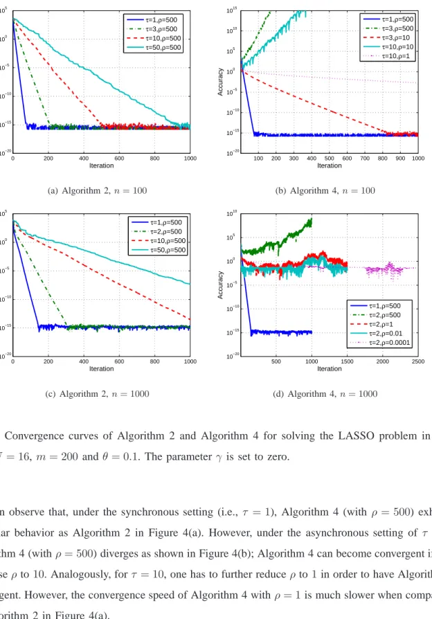
Figure 4(a) and Figure 4(b) respectively display the convergence curves (accuracy versus iteration
number) of Algorithm 2 and Algorithm 4 for solving (52) withN = 16,m= 200,n= 100andθ= 0.1.
The accuracy is defined as
accuracy = |Lρ(x
k,xk
0,λk)−F⋆|
F⋆ (53)
where F⋆ denotes the optimal objective value of problem (52). One can see from Figure 4(a) that
0 200 400 600 800 1000 10−20 10−15 10−10 10−5 100 105 Iteration Accuracy τ=1,ρ=500 τ=3,ρ=500 τ=10,ρ=500 τ=50,ρ=500 (a) Algorithm 2,n= 100 100 200 300 400 500 600 700 800 900 1000 10−20 10−15 10−10 10−5 100 105 1010 1015 Iteration Accuracy τ=1,ρ=500 τ=3,ρ=500 τ=3,ρ=10 τ=10,ρ=10 τ=10,ρ=1 (b) Algorithm 4,n= 100 0 200 400 600 800 1000 10−20 10−15 10−10 10−5 100 105 Iteration Accuracy τ=1,ρ=500 τ=2,ρ=500 τ=10,ρ=500 τ=50,ρ=500 (c) Algorithm 2,n= 1000 500 1000 1500 2000 2500 10−20 10−15 10−10 10−5 100 105 1010 Iteration Accuracy τ=1,ρ=500 τ=2,ρ=500 τ=2,ρ=1 τ=2,ρ=0.01 τ=2,ρ=0.0001 (d) Algorithm 4,n= 1000
Fig. 4: Convergence curves of Algorithm 2 and Algorithm 4 for solving the LASSO problem in (52)
with N = 16, m= 200 andθ= 0.1. The parameterγ is set to zero.
one can observe that, under the synchronous setting (i.e., τ = 1), Algorithm 4 (with ρ = 500) exhibits
a similar behavior as Algorithm 2 in Figure 4(a). However, under the asynchronous setting of τ = 3,
Algorithm 4 (withρ= 500) diverges as shown in Figure 4(b); Algorithm 4 can become convergent if one
decreaseρto10. Analogously, forτ = 10, one has to further reduceρ to1in order to have Algorithm 4
convergent. However, the convergence speed of Algorithm 4 withρ= 1is much slower when comparing
to Algorithm 2 in Figure 4(a).
(52) with n increased to 1000. Note that, given m = 200 and n= 1000, the cost functions fi(wi) ,
kAiwi−bik2 in (52) are no longer strongly convex. One can observe from Figure 4(c) that Algorithm
2 (with ρ= 500, γ = 0) still converges properly for various values ofτ. However, as one can see from
Figure 4(d), Algorithm 4 always diverges for various values of ρ even when the delay τ is as small as
two. As a result, the strong convexity assumed in Theorem 2 may also be necessary in practice. We conclude from these simulation results that Algorithm 2 significantly outperforms Algorithm 4 in the asynchronous network, even though the two have the same convergence behaviors in the synchronous network.
VI. CONCLUDINGREMARKS
In this paper, we have proposed the AD-ADMM (Algorithm 2) aiming at solving large-scale instances of problem (1) over a star computer network. Under the partially asynchronous model, we have shown (in Theorem 1) that the AD-ADMM can deterministically converge to the set of KKT points of problem
(4), even in the absence of convexity offi’s. We have also compared the AD-ADMM (Algorithm 2) with
an alternative asynchronous implementation (Algorithm 4), and illustrated the interesting fact that a slight modification of the algorithm can significantly change the algorithm convergence conditions/behaviors in the asynchronous setting.
From the presented simulation results, we have observed that the AD-ADMM may exhibit linear convergence for some structured instances of problem (1). The conditions under which linear convergence can be achieved are presented in the companion paper [25]. Numerical results which demonstrate the time efficiency of the proposed AD-ADMM on a high performance computer cluster are also presented in [25]. APPENDIXA PROOF OFLEMMA 1 Notice that Lρ(xk+1,xk0+1,λk+1)− Lρ(xk,xk0,λk) =Lρ(xk+1,xk0+1,λk+1)− Lρ(xk+1,xk0,λk+1) +Lρ(xk+1,xk0,λk+1)− Lρ(xk+1,xk0,λk) +Lρ(xk+1,xk0,λk)− Lρ(xk,xk0,λk). (A.1)
We bound the three pairs of the differences on the right hand side (RHS) of (A.1) as follows. Firstly, since −xT 0 PN i=1λki+1+ ρ 2 PN
i=1kxki+1−x0k2+ γ2kx0−xk0k2 in (25) is strongly convex with respect
to (w.r.t.)x0 with modulusγ +N ρ, by [34, Definition 2.1.2], we have
−(xk 0)T N X i=1 λk+1 i + ρ 2 N X i=1 kxk+1 i −x k 0k2 − −(xk+1 0 )T N X i=1 λk+1 i + ρ 2 N X i=1 kxk+1 i −x k+1 0 k2+ γ 2kx k+1 0 −xk0k2 ≥ − N X i=1 λk+1 i +ρ N X i=1 (xk+1 0 −xki+1) +γ(xk+1 0 −xk0) T (xk 0−xk0+1) + γ+N ρ 2 kx k+1 0 −xk0k2. (A.2)
By the optimality condition of (25) and the convexity of h, we respectively have
sk+1 0 − N X i=1 λk+1 i +ρ N X i=1 (xk+1 0 −xki+1) +γ(xk+1 0 −xk0) T (xk 0 −xk0+1)≥0, (A.3) h(xk 0)≥h(xk0+1) + (sk0+1)T(xk0−xk0+1). (A.4)
By subsequently applying (A.3) and (A.4) to (A.2), we obtain
h(xk 0)−(xk0)T N X i=1 λk+1 i + ρ 2 N X i=1 kxk+1 i −x k 0k2 − h(xk+1 0 )−(xk0+1)T N X i=1 λk+1 i +ρ 2 N X i=1 kxk+1 i −x k+1 0 k2+ γ 2kx k+1 0 −xk0k2 ≥ γ+N ρ 2 kx k+1 0 −xk0k2, (A.5) that is, Lρ(xk+1,xk0+1,λk+1)− Lρ(xk+1,xk0,λk+1) ≤ −2γ+2N ρkxk+1 0 −xk0k2. (A.6)
Secondly, it directly follows from (26) that Lρ(xk+1,xk0,λk+1)− Lρ(xk+1,xk0,λk) = N X i=1 (λk+1 i −λ k i)T(xki+1−x k 0) = X i∈Ak (λk+1 i −λ k i)T(xki+1−x ¯ ki+1 0 ) + X i∈Ak (λk+1 i −λ k i)T(x ¯ ki+1 0 −xk0) = 1 ρ X i∈Ak kλk+1 i −λ k ik2 + X i∈Ak (λk+1 i −λki)T(x ¯ ki+1 0 −xk0), (A.7)
where the second equality is due to the fact that λk+1
i =λki ∀i∈ Ack and the last equality is obtained
by applying λk+1 i =λki +ρ(xki+1−x ¯ ki+1 0 ) ∀i∈ Ak (A.8) as shown in (24). Thirdly, define Li(xi,xk0,λk) = fi(xi) + xTi λki + ρ
2kxi −xk0k2 and assume that ρ ≥ L. Since,
by [34, Lemma 1.2.2], the minimum eigenvalue of the Hessian matrix of fi(xi) is no smaller than −L,
Li(xi,xk0,λk)is strongly convex w.r.t.xiand the convexity parameter is given byρ−L≥09. Therefore,
one has Li(xki,xk0,λk)≥ Li(xki+1,xk0,λk) + (∇fi(xki+1) +λki +ρ(xik+1−xk0))T(xki −xki+1) +ρ−L 2 kx k+1 i −x k ik2. (A.9)
Also, by the optimality condition of (23), one has,∀i∈ Ak,
0=∇fi(xk+1 i ) +λ k i +ρ(xki+1−x ¯ ki+1 0 ) (A.10) = (∇fi(xki+1) +λik+ρ(xki+1−xk0)) +ρ(xk0 −x¯ki+1 0 ). (A.11) 9Whenf
iis a convex function, the minimum eigenvalue of the Hessian matrix offi(xi)is zero. So, the convexity parameter ofLi(xi,λ
k
By substituting (A.11) into (A.9) and by (26), we have Lρ(xk+1,xk0,λk)− Lρ(xk,xk0,λk) = N X i=1 (Li(xki+1,λk,xk0)− Li(xki,λk,xk0)) = X i∈Ak (Li(xki+1,λk,xk0)− Li(xki,λk,xk0)) ≤ −ρ−L 2 X i∈Ak kxk+1 i −xkik2 +ρ X i∈Ak (xk¯i+1 0 −xk0)T(xki+1−x k i), (A.12)
where the second equality is due to xk+1
i =xki ∀i∈ Ack from (23).
After substituting (A.6), (A.7) and (A.12) into (A.1), we obtain Lρ(xk+1,xk0+1,λk+1)− Lρ(xk,xk0,λk) ≤ −2γ+2N ρkxk+1 0 −xk0k2+ 1 ρ X i∈Ak kλk+1 i −λ k ik2 −ρ−2LX i∈Ak kxk+1 i −x k ik2 +X i∈Ak (λk+1 i −λki)T(x ¯ ki+1 0 −xk0) +ρX i∈Ak (x¯ki+1 0 −xk0)T(xki+1−x k i). (A.13)
Recall the Young’s inequality, i.e.,
aTb≤ 1
2δkak
2+δ
2kbk
2, (A.14)
for anya, bandδ >0, and apply it to the fourth and fifth terms in the RHS of (A.13) with δ= 1 and
APPENDIXB PROOF OFLEMMA 2 It is easy to show that
k X j=0 X i∈Aj kxj 0−x ¯ ji+1 0 k2 = k X j=0 X i∈Aj k j−1 X ℓ=¯ji+1 (xℓ 0−xℓ0+1)k2 ≤ k X j=0 X i∈Aj (j−¯ji−1) j−1 X ℓ=¯ji+1 kxℓ 0−xℓ0+1k2 ≤ k X j=0 X i∈Aj (τ −1) j−1 X ℓ=j−τ+1 kxℓ0−xℓ+1 0 k2 ≤S(τ −1) k X j=0 j−1 X ℓ=j−τ+1 kxℓ0−xℓ+1 0 k2 (A.15)
where, in the second inequality, we have applied the fact of j −τ ≤ ¯ji < j from (21); in the last
inequality, we have applied the assumption of |Ak| < S for all k. Notice that, in the summation
Pk j=0 Pj−1 ℓ=j−τ+1kxℓ0 −xℓ0+1k2, each kx j 0 −x j+1
0 k2, where j = 0, . . . , k−1, appears no more than
τ −1 times. Thus, one can upper bound
k X j=0 j−1 X ℓ=j−τ+1 kxℓ0−xℓ+1 0 k2 ≤(τ−1) k−1 X j=0 kxj+1 0 −x j 0k2, (A.16)
which, combined with (A.15), yields (32).
APPENDIXC
PROOF OFLEMMA 3
The proof is similar to [18, Lemma 2.3]. We present the proof here for completeness. By recalling equation (29) and applying it to (26), one obtains
Lρ(xk+1,xk0+1,λk+1) =h(xk0+1) + N X i=1 fi(xki+1) − N X i=1 (∇fi(xki+1))T(xki+1−xk0+1) + ρ 2 N X i=1 kxk+1 i −x k+1 0 k2. (A.17)
As ∇fi is Lipschitz continuous under Assumption 2, the descent lemma [36, Proposition A.24] holds
fi(xk0+1)≤fi(xki+1) + (∇fi(xki+1))T(x0k+1−xki+1)
+L
2kx
k+1
By combining (A.17) and (A.18), one can lower bound Lρ(xk+1,x0k+1,λk+1) as Lρ(xk+1,xk0+1,λk+1)≥h(xk0+1) + N X i=1 fi(xk0+1) +ρ−L 2 N X i=1 kxk+1 i −x k+1 0 k2, (A.19)
which implies (33) given ρ≥L and under Assumption 2.
APPENDIXD PROOF OFTHEOREM 2
For ease of analysis, we equivalently write Algorithm 4 as follows: For iteration k= 0,1, . . . ,
xk+1 i = arg min xi fi(xi) +xTi λ ¯ ki+1 i + ρ 2kxi−x ¯ ki+1 0 k2, ∀i∈ Ak xk i ∀i∈ Ack , (A.20) xk+1 0 = arg minx0 h(x0)−xT0 PN i=1λki + ρ 2 PN i=1kxki+1−x0k2, (A.21) λk+1 i =λ k i +ρ(xki+1−x k+1 0 ) ∀i∈ V. (A.22)
Here, k¯i is the last iteration number for which the master node receives message from worker i ∈ Ak
before iterationk. Fori∈ Ac
k, let us denoteeki (k−τ <eki< k) as the last iteration number for which the
master node receives message from workeribefore iterationk, and further denotebki (eki−τ ≤bki <eki)
as the last iteration number for which the master node receives message from worker ibefore iteration
e
ki. Then, by (A.20), it must be
xeki+1 i = arg minx i fi(xi) +xTi λ b ki+1 i + ρ 2kxi−x b ki+1 0 k2 ∀i∈ Ack, (A.23) xk+1 i =x e ki+1 i , (A.24)
where the second equation is due to xeki+1
i =x
e ki+2
i =· · ·=xki =xik+1 ∀i∈ Ack.
Let us consider the following update steps
xk+1 i = arg min xi αfi(xi) +xTi λe ¯ ki+1 i + β 2kxi−x ¯ ki+1 0 k2, ∀i∈ Ak arg min xi αfi(xi) +xTi λe b ki+1 i + β 2kxi−x b ki+1 0 k2 ∀i∈ Ack , (A.25) xk+1 0 = arg minx 0 αh(x0)−xT 0 PN i=1λeki + β 2 PN i=1kx k+1 i −x0k2, (A.26) e λk+1 i =λe k i +β(xki+1−x k+1 0 ) ∀i∈ V, (A.27)
where α, β >0. One can verify that (A.25)-(A.27) are equivalent to (A.20)-(A.22) and (A.23)-(A.24) if
We first consider the optimality condition of (A.25) for i∈ Ak: 0≥α∂fi(xki+1)T(xki+1−x⋆i) + (λe ¯ ki+1 i +β(x k+1 i −x ¯ ki+1 0 ))T(xki+1−x ⋆ i) =α∂fi(xki+1) T(xk+1 i −x ⋆ i) + (λeki+1) T(xk+1 i −x ⋆ i) + (λek¯i+1 i −λe k i)T(xki+1−x ⋆ i) +β(xk0+1−x ¯ ki+1 0 )T(xki+1−x ⋆ i), (A.28)
where we have applied (A.27) to obtain the equality. Since, under Assumption 3,fi is strongly convex,
one has αfi(x⋆i)≥αfi(xki+1) +α∂fi(xki+1)T(x⋆i −xki+1) + ασ2 2 kx k+1 i −x ⋆ ik2. (A.29)
Combining (A.28) and (A.29) gives rise to
αfi(xki+1)−αfi(x⋆i) +λeTi (xki+1−x ⋆ i) + ασ2 2 kx k+1 i −x ⋆ ik2 + (λek+1 i −λei) T(xk+1 i −x ⋆ i) + (λe ¯ ki+1 i −λe k i)T(xki+1−x ⋆ i) +β(xk+1 0 −x ¯ ki+1 0 )T(xki+1−x⋆i)≤0 ∀i∈ Ak. (A.30)
On the other hand, consider the optimality condition of (A.25) for i∈ Ac
k: 0≥α∇fi(xki+1)T(xki+1−x⋆i) + (λe b ki+1 i +β(xki+1−x b ki+1 0 ))T(xki+1−x⋆i) =α∇fi(xki+1)T(xki+1−x⋆i) + (λebki+1 i +λe e ki+1 i −λe e ki i −β(x e ki+1 i −x e ki+1 0 ) +β(x e ki+1 i −x b ki+1 0 ))T(xki+1−x⋆i) =α∇fi(xki+1) T(xk+1 i −x ⋆ i) + (λe e ki+1 i ) T(xk+1 i −x ⋆ i) + (λebki+1 i −λe e ki)T(xk+1 i −x⋆i) +β(x e ki+1 0 −x b ki+1 0 )T(xki+1−x⋆i), (A.31)
where (A.27) with k = eki and (A.24) are used to obtain the first equality. By combining (A.29) with
(A.31), one obtains
αfi(xki+1)−αfi(x⋆i) +λeTi (xki+1−x ⋆ i) + ασ2 2 kx k+1 i −x ⋆ ik2 + (λeeki+1 i −λei)T(xik+1−x⋆i) + (λe b ki+1 i −λe e ki)T(xk+1 i −x⋆i) +β(xeki+1 0 −x b ki+1 0 )T(xki+1−x ⋆ i)≤0 ∀i∈ Ack. (A.32)
terms, we obtain that α N X i=1 fi(xki+1)−α N X i=1 fi(x⋆i) + N X i=1 e λTi (xk+1 i −x ⋆ i) + N X i=1 ασ2 2 kx k+1 i −x ⋆ ik2 + X i∈Ak (λek+1 i −λei) T(xk+1 i −x ⋆ i) + X i∈Ac k (λeeki+1 i −λei) T(xk+1 i −x ⋆ i) | {z } (a) + X i∈Ak (λek¯i+1 i −λe k i)T(xki+1−x ⋆ i) + X i∈Ac k (λebki+1 i −λe e ki)T(xk+1 i −x ⋆ i) + X i∈Ak β(xk+1 0 −x ¯ ki+1 0 )T(xki+1−x⋆i) + X i∈Ac k β(xeki+1 0 −x b ki+1 0 )T(xki+1−x⋆i) | {z } (b) ≤0. (A.33)
The term (a) in (A.33), after adding and subtractingPi∈Ac
k( e λk+1 i −λei)T(xik+1−x⋆i), can be written as (a) = N X i=1 (λek+1 i −λei)T(xki+1−x ⋆ i) + X i∈Ac k (λeeki+1 i −λe k+1 i ) T(xk+1 i −x ⋆ i). (A.34)
The term (b) in (A.33) can be expressed as
(b) = X i∈Ak β(xk+1 0 −xk0 +xk0−x ¯ ki+1 0 )T(xki+1−x⋆i) + X i∈Ac k β(xeki+1 0 −x b ki+1 0 )T(xki+1−x⋆i) = N X i=1 β(xk+1 0 −xk0)T(xki+1−x ⋆ i) + X i∈Ac k β(xeki+1 0 −x b ki+1 0 −xk0+1+x0k)T(xki+1−x ⋆ i) + X i∈Ak β(xk 0−x ¯ ki+1 0 )T(xki+1−x⋆i). (A.35)
Note that, by applying (A.27) and the fact of x⋆
i =x⋆0 ∀i∈ V, one can write
N X i=1 β(xk+1 0 −xk0)T(xki+1−x ⋆ i) = N X i=1 β(xk+1 0 −xk0)T(xki+1−x k+1 0 +xk0+1−x⋆i) = N X i=1 (xk+1 0 −xk0)T(λeik+1−λeki) +N β(xk0+1−xk0)T(xk0+1−x⋆0). (A.36) So, The term (b) in (A.35) is given by
(b) = N X i=1 (xk+1 0 −xk0)T(λeki+1−λe k i) +N β(xk0+1−xk0)T(xk0+1−x⋆0) + X i∈Ac k β(xeki+1 0 −x b ki+1 0 −xk0+1+x0k)T(xki+1−x ⋆ i) + X i∈Ak β(xk0−x¯ki+1 0 )T(xki+1−x ⋆ i). (A.37)
It can be shown that N X i=1 (xk+1 0 −xk0)T(eλki+1−λe k i)≥0. (A.38)
To see this, consider the optimality condition of (A.26): ∀x0∈Rn,
0≥αh(xk+1 0 )−αh(x0)− N X i=1 (λeki +β(xk+1 i −x k+1 0 ))T(xk0+1−x0) =αh(xk+1 0 )−αh(x0)− N X i=1 (λek+1 i ) T(xk+1 0 −x0), (A.39)
where the equality is due to (A.27). By lettingx0 =xk
0 in (A.39) and also considering (A.39) for iteration
k andx0 =xk+1 0 , we have 0≥αh(xk+1 0 )−αh(xk0)− N X i=1 (eλk+1 i ) T(xk+1 0 −xk0), 0≥αh(xk 0)−αh(xk0+1)− N X i=1 (eλki)T(xk 0−xk0+1), (A.40)
respectively. By summing the above two equations, we obtain (A.38). Moreover, by lettingx0=x⋆
i =x⋆0 in (A.39), we have αh(xk+1 0 )−αh(x⋆0)− N X i=1 e λT i (xk0+1−x⋆i)− N X i=1 (λek+1 i −λei)T(x0k+1−x⋆i)≤0. (A.41)
By summing (A.41) and (A.33) followed by applying (A.34), (A.37) and (A.38), one obtains
α N X i=1 fi(xki+1) +αh(x k+1 0 )−α N X i=1 fi(x⋆i)−αh(x⋆0) + N X i=1 e λTi (xk+1 i −x k+1 0 ) + N X i=1 ασ2 2 kx k+1 i −x ⋆ ik2 + 1 β N X i=1 (λek+1 i −λei)T(eλik+1−λeki) +N β(xk0+1−xk0)T(xk0+1−x⋆0) + X i∈Ac k (eλeki+1 i −λe k+1 i +λe b ki+1 i −λe e ki)T(xk+1 i −x ⋆ i) + X i∈Ak (λek¯i+1 i −λe k i)T(xki+1−x ⋆ i) + X i∈Ac k β(xeki+1 0 −x b ki+1 0 −xk0+1+x0k)T(xki+1−x ⋆ i) + X i∈Ak β(xk 0−x ¯ ki+1 0 )T(xki+1−x ⋆ i)≤0, (A.42) where the seventh term in the LHS is obtained by applying (A.27).
We sum (A.42) for k= 0, . . . , K−1 and take the average, which yields α K KX−1 k=0 XN i=1 fi(xki+1) +h(xk0+1) −α XN i=1 fi(x⋆i) +h(x⋆0) + 1 K KX−1 k=0 N X i=1 e λT i (xki+1−xk0+1) + 1 βK KX−1 k=0 N X i=1 (λek+1 i −λei)T(λeki+1−λe k i) | {z } (a) +N β K KX−1 k=0 (xk+1 0 −xk0)T(xk0+1−x⋆0) | {z } (b) ≤ −1 K KX−1 k=0 N X i=1 ασ2 2 kx k+1 i −x ⋆ ik2 + 1 K KX−1 k=0 − X i∈Ac k (λeeki+1 i −λe k+1 i +λe b ki+1 i −λe e ki)T(xk+1 i −x⋆i)− X i∈Ak (λe¯ki+1 i −λeki)T(xki+1−x⋆i) | {z } (c) + 1 K KX−1 k=0 − X i∈Ac k β(xeki+1 0 −x b ki+1 0 −xk0+1+x0k)T(xki+1−x ⋆ i)− X i∈Ak β(xk 0 −x ¯ ki+1 0 )T(xki+1−x ⋆ i) | {z } (d) . (A.43) It is easy to see that term (a)
(a) = 1 2 KX−1 k=0 kλek+1 i −λeik2− keλki −λeik2+kλeki+1−λekik2 = 1 2kλe K i −λeik2− 1 2kλe 0 i −λeik2+ 1 2 KX−1 k=0 kλek+1 i −λe k ik2, (A.44)
and similarly, term (b)
(b) = 1 2 KX−1 k=0 kxk+1 0 −x⋆0k2− kxk0−x0⋆k2+kxk0+1−xk0k2 = 1 2kx K 0 −x⋆0k2− 1 2kx 0 0−x⋆0k2+ 1 2 KX−1 k=0 kxk+1 0 −xk0k2. (A.45)
Notice that one can bound the term PKk=0−1Pi∈Ak(λek¯i+1 i −λeki)T(xki+1−x⋆i) in (c) as follows KX−1 k=0 X i∈Ak (λe¯ki+1 i −λeki)T(xki+1−x⋆i) = KX−1 k=0 X i∈Ak k−1 X ℓ=¯ki+1 (λeℓ i −λeℓi+1)T(xki+1−x⋆i) ≤ KX−1 k=0 X i∈Ak k−1 X ℓ=k−τ+1 kλeℓ i−eλℓi+1k · kxki+1−x⋆ik ≤ N X i=1 KX−1 k=0 k−1 X ℓ=k−τ+1 1 2β2kλe ℓ i −λeℓi+1k2+ β2 2 kx k+1 i −x⋆ik2 (A.46) ≤ N X i=1 KX−1 k=0 τ−1 2β2 kλe k+1 i −λekik2+ (τ −1)β2 2 kx k+1 i −x⋆ik2 , (A.47)
where the second inequality is obtained by applying the Young’s inequality:
aTb≤ 1
2δkak
2+δ
2kbk
2 (A.48)
for any a, b and δ > 0; the last inequality is caused by the fact that the term kλek+1
i −λekik2 for each
k does not appear more than τ −1 times in the RHS of (A.46). By applying a similar idea to the first
term of (c) and by (A.47), one eventually can bound (c) as follows
(c)≤ 3(τ −1) 2β2 N X i=1 KX−1 k=0 kλek+1 i −eλkik2+ 3(τ −1)β2 2 N X i=1 KX−1 k=0 kxk+1 i −x⋆ik2. (A.49)
Similarly, the term PKk=0−1Pi∈Akβ(xk
0−x
¯
ki+1
0 )T(xki+1−x⋆i) in (d) can be upper bounded as follows
KX−1 k=0 X i∈Ak β(xk 0 −x ¯ ki+1 0 )T(xki+1−x⋆i)≤ KX−1 k=0 X i∈Ak k−1 X ℓ=k−τ+1 βkxk 0 −x ¯ ki+1 0 k · kxki+1−x⋆ik ≤ N X i=1 KX−1 k=0 k−1 X ℓ=k−τ+1 1 2kx k+1 0 −xk0k2+ β2 2 kx k+1 i −x ⋆ ik2 (A.50) ≤ N X i=1 KX−1 k=0 τ−1 2 kx k+1 0 −xk0k2+ (τ −1)β2 2 kx k+1 i −x⋆ik2 . (A.51)
By applying a similar idea to the first term of (d) and by (A.51), one can bound (d) as follows
(d)≤ N X i=1 KX−1 k=0 τkxk+1 0 −xk0k2+τ β2kxki+1−x⋆ik2 . (A.52)
After substituting (A.44), (A.45), (A.49) and (A.52) into (A.43), we obtain that α XN i=1 fi( ¯xKi ) +h( ¯xK0 ) −α XN i=1 fi(x⋆i) +h(x⋆0) + N X i=1 e λT i( ¯xKi −x¯K0 ) ≤ Kα KX−1 k=0 XN i=1 fi(xki+1) +h(xk0+1) −α XN i=1 fi(x⋆i) +h(x⋆0) + 1 K KX−1 k=0 N X i=1 e λTi (xk+1 i −x k+1 0 ) ≤ 1 2βK N X i=1 kλe0i −λeik2− 1 2βK N X i=1 kλeKi −λeik2+N β 2Kkx 0 0−x⋆0k2− N β 2Kkx K 0 −x⋆0k2 + 3(τ −1) 2Kβ2 − 1 2βK XN i=1 KX−1 k=0 kλek+1 i −λekik2+ N τ K − N β 2K KX−1 k=0 kxk+1 0 −xk0k2 + 1 K KX−1 k=0 N X i=1 3(τ −1)β2+ 2τ β2−ασ2 2 kxk+1 i −x ⋆ ik2 (A.53)
where the first inequality is by the convexity of fi’s and h.
According to (A.53), by choosing
β≥max{2τ,3(τ −1)}, α≥ (5τ −3)β
2
σ2 , (A.54)
and recalling that λi =λei/α andρ=β/α, one can obtain
XN i=1 fi( ¯xKi ) +h( ¯xK0 ) − XN i=1 fi(x⋆i) +h(x⋆0) + N X i=1 λT i ( ¯xKi −x¯K0 ) ≤ 2ρK1 N X i=1 kλ0i −λik2+N ρ 2Kkx 0 0−x⋆0k2. (A.55)
Note that (A.54) is equivalent to
ρ=β/α≤ σ 2 (5τ −3)β ≤ σ2 (5τ−3) max{2τ,3(τ −1)}. (A.56) Now, let λi =λ⋆ i + ¯ xKi −x¯K0
kx¯Ki −x¯K0k ∀i∈ V in (A.57), and note that, by the duality theory [37], XN i=1 fi( ¯xKi ) +h( ¯xK0 ) − XN i=1 fi(x⋆i) +h(x⋆0) + N X i=1 (λ⋆i)T( ¯xKi −x¯K 0 )≥0.
Thus, we obtain that
N X i=1 kx¯Ki −x¯K 0 k ≤ 1 K 1 2ρkmaxak≤1 XN i=1 kλ0i −λ⋆i +ak2 +N ρ 2 kx 0 0−x⋆0k2 , C1 K. (A.57)