On the optimism correction of the area under the
receiver operating characteristic curve in logistic
prediction models
Amaia Iparragirre∗,1, Irantzu Barrio1,3and Mar´ıa Xos´e Rodr´ıguez- ´Alvarez2,4
Abstract
When the same data are used to fit a model and estimate its predictive performance, this estimate may be optimistic, and its correction is required. The aim of this work is to compare the behaviour of different methods proposed in the literature when correcting for the optimism of the estimated area under the receiver operating characteristic curve in logistic regression models. A simulation study (where the theoretical model is known) is conducted considering different number of covari-ates, sample size, prevalence and correlation among covariates. The results suggest the use of
k-fold cross-validation with replication and bootstrap.
MSC: 62J99.
Keywords: Prediction models, logistic regression, area under the receiver operating characteristic
curve, validation, bootstrap.
1. Introduction
Prediction models play an important role in daily clinical practice. They provide clin-icians with a tool to identify individuals at higher risk, and thus help in the decision making process. The development of risk prediction models for patients with diseases such as breast cancer (Wishart et al., 2012), chronic obstructive pulmonary disease (Quintana et al., 2014), or heart failure (Garcia-Gutierrez et al., 2017), among others, has increased during the last years. Once a model is developed, the aim is generally to apply it on new patients. Thus, a good but accurate predictive (or generalisation)
∗Corresponding author: [email protected]. Address: Departamento de Matem´atica Aplicada, Estad´ıstica e Investigaci´on Operativa. Facultad de Ciencia y Tecnolog´ıa. Universidad del Pa´ıs Vasco UPV/EHU. Barrio Sarriena s/n. 48940 Leioa.
1Departamento de Matem´atica Aplicada, Estad´ıstica e Investigaci´on Operativa. Universidad del Pa´ıs Vasco
UPV/EHU.
2BCAM-Basque Center for Applied Mathematics, Bilbao, Spain.
3Red de Investigaci´on en Servicios de Salud en Enfermedades Cr´onicas (REDISSEC). 4IKERBASQUE, Basque Foundation for Science, Bilbao, Spain.
Received: February 2018 Accepted: January 2019
model performance is required. This work focuses on logistic regression models. In this setting, there are different ways to evaluate the performance, including calibration and discrimination measures (Steyerberg, 2009). Calibration refers to the agreement between observed outcomes or responses and predictions, while discrimination is con-cerned with the ability of the model to discriminate between individuals with and with-out the characteristic of interest. The area under the receiver operating characteristic (ROC) curve (Bamber, 1975; Hanley and McNeil, 1982; Swets, 1988), on which this work is focused, is a measure of discrimination.
It is well known that if in the development process of a prediction model, the same data is used to, first, fit the model and, then, evaluate its performance, this estimate, usually referred to as apparent or re-substituted performance, could be optimistic (see, e.g., Efron, 1986; Copas and Corbett, 2002). This is a consequence of the fact that most model fitting strategies rely on optimality criteria for the data used. Thus, in or-der to guarantee the model’s usefulness when applied to new patients, the validation or correction of this optimism is required. Arguably, the best strategy to estimate the generalisation model performance is to apply it to new data. That is to say, the per-formance of the model is estimated based on individuals (observations) that have not been used in the model derivation/development process. This strategy is called external validation. Unfortunately, in practice this is usually not feasible. Most of the times it is not possible to obtain new data for that purpose due to difficulty or expense in their collection. To overcome the problem, different approaches have been proposed in the literature with the aim of estimating the performance of a model internally, i.e., re-using the data where the model has been derived/fitted. Split-sample validation (Picard and Berk, 1990; Snee, 1977) is possibly the most commonly used method in medical re-search. However, especially for small sample sizes, it has shown to provide pessimistic (over-corrected) estimates of the performance with a large variance (see, e.g., Steyerberg et al., 2001; Austin and Steyerberg, 2017). Therefore, alternative approaches to split-sample validation, such ask-fold cross-validation or bootstrap techniques, have been suggested (Stone, 1974; Efron, 1983; Harrell, Lee and Mark, 1996).
For the specific case of binary outcomes (as is the case of this paper), the literature contains several papers comparing different methods for correcting the optimism of the apparent area under the ROC curve (AUC). Important references are Harrell (2001); Steyerberg et al. (2001, 2003); Airola et al. (2011); Smith et al. (2014); Austin and Steyerberg (2017). For instance, Airola et al. (2011) compare different cross-validation techniques for estimating the AUC and propose the leave-pair-out cross-validation as the preferred method for optimism correction. To a similar conclusion comes Smith et al. (2014), who focus on small data sets. Yet, other authors recommend the use of bootstrapping (e.g., Smith et al., 2014; Steyerberg et al., 2001; Austin and Steyerberg, 2017). The papers by Steyerberg et al. (2001, 2003); Smith et al. (2014) and Austin and Steyerberg (2017) all focus on logistic regression models. In particular, all these papers study the impact of different values of events per variable (EPV) on the performance of several correction methods by means of simulations based on a large real data set.
EPV is defined by the ratio of the number of events (i.e., the number of observations in the smaller of the two groups of the binary outcome), relative to the number of re-gression coefficients in the model (see e.g., van Smeden et al., 2018). In most of the above-mentioned papers, simulations are done with a fixed number of covariates. Nev-ertheless, in practice other factors beyond the EPV may impact the performance of the methods, such as a) the number of covariates in the model, b) the available sample size, c) the prevalence; and/or d) the correlation among covariates. The number of covari-ates, sample size and prevalence are all together related to the EPV, but the last two are imposed by the available data. It has been reported that the bias of the apparent model performance estimate increases as the number of covariates increases (Hastie, Tibshirani and Friedman, 2001; Copas and Corbett, 2002). However, to the best of our knowledge there is a lack of studies comparing different correction methods in terms of the number of covariates. Hence, the primary aim of this study is to empirically evaluate the effect that the increase of the number of covariates may have on the performance of different methods (including split-sample, cross-validation and bootstrap) for the correction of the apparent AUC. In addition, we study the impact of the correlation among covari-ates as well as the prevalence of the disease and the sample size. Finally, in contrast to the above-mentioned studies, we conduct a simulation study in a situation where the theoretical logistic regression model is known.
The rest of the paper is organised as follows. Section 2 outlines the optimism cor-rection methods that have been considered in this work. In Section 3 the simulation study conducted to analyse the performance of the optimism correction methods is de-scribed. Additionally, the results obtained are reported. Finally, the paper closes with a discussion in Section 4.
2. Methods
This section introduces the needed notation and background and describes the different methods that have been considered throughout this study to correct for the optimism of the apparent AUC. Recall that we denote as apparent AUC that which is obtained when all the available data are used to, first, fit the model and then, estimate the AUC.
2.1. Notation and preliminaries
Consider a collection ofpcovariates denoted by the vectorXXX= (1,X1,X2, . . . ,Xp) T
, and letDbe the random variable denoting the presence (D=1) or absence (D=0) of the characteristic of interest (e.g., a certain disease). Letp(xxx) =P(D=1|XXX=xxx)denote the conditional probability of being diseased for a patient with a vector of covariate values
The specific form of the logistic regression model is: p(xxx) = e β0+β1x1+...+βpxp 1+eβ0+β1x1+...+βpxp = eβββTxxx 1+eβββTxxx ∈(0,1), (1) whereβββ= (β0, . . . ,βp) T
is the vector of (unknown) regression coefficients. Let us as-sume that we have a sample of independent and identically distributed (i.i.d.) observa-tions{(xxxi,di)}
n
i=1from population(XXX,D), and denote as ˆβββˆˆ = (βˆ0, . . . ,βˆp)Tthe maximum likelihood estimator ofβββ(Hosmer and Lemeshow, 2000; McCullagh and Nelder, 1989). The estimated probabilities of being diseased for each individual in the sample can be thus calculated as follows (see (1)):
ˆ
p(xxxi) =
eβββˆTxxxi
1+eβββˆTxxxi (i=1, . . . ,n). (2)
2.2. Discriminative ability
As said in the Introduction, this paper focuses on the AUC. The AUC ranges from 0.5 (in the case of an uninformative model) to 1 (a perfect model), and it is frequently estimated by the Mann-Whitney U-statistic (Bamber, 1975; Hanley and McNeil, 1982; Pepe, 2003). More precisely, for the specific case of the logistic regression model, we have d AUC= 1 n0·n1 X j∈D0 X k∈D1 [I(pˆ(xxxj)<pˆ(xxxk)) +0.5I(pˆ(xxxj) =pˆ(xxxk))], (3)
whereD0andD1are the index sets forD=0 andD=1, respectively andn0andn1their
respective sizes. Note that expression (3) corresponds to the so-called apparent AUC, since all data are used for its calculation.
2.3. Optimism correction methods
2.3.1. Split-sample validation
In split-sample validation, the available sample{(xxxi,di)}ni=1 is randomly divided into
two subsamples, a derivation sample xxxderl ,dlder nder
l=1
and a validation sample xxxvalm ,
dval m
nval m=1
, withn=nder+nval. Typically, the sample is split into two subsamples of the same size(1/2 : 1/2)(Snee, 1977). Split-sample validation proceeds as follows. A logistic regression model is fitted to the derivation sample and the regression coefficients are estimated. These regression coefficients are used to estimate the predicted probabil-ities for the individuals in the validation sample following expression (2), which then are further used to calculate the corrected AUC by means of equation (3).
2.3.2. K-fold cross-validation
This method consists in splitting the available sample intok subsamples of (approxi-mately) the same size. In pretty much the same way as split-sample validation, k−1 subsamples are considered as the derivation sample, and the remainder is used as vali-dation sample to estimate the AUC. In contrast, however, to split-sample, the process is repeatedktimes, leaving-out one different subsample every time as validation sample. Finally, the corrected AUC is the average of thesekestimated AUCs.
K-fold cross-validation with replication is another variant of this method (see, e.g., Smith et al., 2014). The process explained above is repeatedr times, with a different
k-split of the sample each time. Finally, the corrected AUC is the average of r×k
estimated AUCs.
We would like to note that the describedk-fold cross-validation method is usually referred in the literature, for obvious reasons, as the averaging strategy in contrast to the pooling strategy (see, e.g., Bradley, 1997). In the later, predicted probabilities are calculated in each validation sample, which are then pooled and used to estimate the corrected AUC. This work focuses on the averaging strategy, as it has shown a better performance in previous studies (Parker, G¨unter and Bedo, 2007; Airola et al., 2011). In particular, the averaging strategy does not suffer from the pessimism that occurs when pooling, and it is not affected by the so-called stratification bias. These results have also been corroborated in our setting (results not shown). However, averaging presents a problem that pooling does not have. If the number of diseased (or healthy) individuals is low (or the sample size small), it may happen that some folds will have few individuals (or even none) of the underrepresented group. This will impact the estimate of the AUC when these folds are used as the validation samples, which in turn can lead to a high variance in the estimates of the corrected AUC (Airola et al., 2011).
2.3.3. Leave-one-out cross-validation
In leave-one-out cross-validation, a single observation is omitted from the original sam-ple. The logistic regression model is fitted to the remaining observations (derivation sample). Then, the fitted model is applied on the omitted observation and its predicted probability is estimated (see equation (2)). The process is repeatedntimes (wherenis the size of the original sample), leaving-out one different observation every time. Fi-nally, the AUC corrected by leave-one-out cross-validation method is calculated based on the estimated predicted probabilities of all individuals (see, e.g., Airola et al., 2011; Lachenbruch and Mickey, 1968).
2.3.4. Bootstrap validation
Another possibility to correct for the optimism of the AUC is to use bootstrap techniques (Efron and Tibshirani, 1993). This method can be summarised as follows:
Step 1. Fit the logistic regression model to the original sample{(xxxi,di)} n
i=1and estimate
the apparent AUC, sayAUCdapp.
Forb=1,2, . . . ,B(whereBis the number of bootstrap resamples):
Step 2. Generate a bootstrap resample xxxbi,dib ni=1, of the same size as the original sample, by resampling with replacement from the original sample.
Step 3. Fit a logistic regression model to the bootstrap resample, and estimate its ap-parent AUC, sayAUCdbboot.
Step 4. Apply the fitted logistic regression model in Step 3. on the original sample, calculate the predicted probabilities for each observation and estimate the AUC. LetAUCdbobe this estimate.
The optimism is estimated as follows:
b O= 1 B B X b=1
(AUCdbboot−AUCd
b o),
and the corrected AUC is:AUCdbootstrap=AUCdapp−Ob.
3. Simulation study
This section describes and presents the results of the simulation study conducted to eval-uate the behaviour of the correction methods discussed in Section 2.3.. Specifically, the aim of the study was to compare the AUC estimates provided by the different methods (including the apparent AUC) against the “true” out-of-sample AUC associated with the derived logistic regression model. The “true” out-of-sample AUC refers to the true dis-criminatory capacity of the derived/fitted model when applied to new data or subjects. A variety of factors that could impact the performance of the methods were considered in this study, such as, the number of covariates in the model, the available sample size, the prevalence of the disease (i.e.,prev=P(D=1)) and the correlation among covariates. The steps of the simulation study are described in detail in next section.
3.1. Scenarios and set-up
For a given number of covariates, say,p, the steps of the simulation study can be sum-marised as follows:
Step 1. Generate two independent samples
n xxx(ip)∗,di∗ on i=1 and n xxx(lp)∗∗,d∗∗l oN l=1 of
re-spectively size n and N (the superscript (p) is used to emphasise the covariate vector length) as follows:
Step 1.1 Generateηi ∼Bernoulli(prev), and generate the covariate vector value xxx(ip)∗ xxx(ip)∗∼Nµµµ(Dp) 0,ΣΣΣ (p) if η i=0, xxx(ip)∗∼N µµµ(Dp) 1,ΣΣΣ (p) if η i=1. (4)
By simulating the covariates in this way, the logistic regression model holds, and the true value of the regression coefficient vectorβββ(p)is known (see Ap-pendix A). This vector is used inStep 1.2below.
Step 1.2 Calculate p(xxx(ip)∗)using equation (1). Step 1.3 Generatedi∗∼Bernoulli(p(xxx(ip)∗)). (To generate
n
xxx(lp)∗∗,dl∗∗ oN
l=1we followed the same steps. We note that this sample
is used inStep 3. to estimate the out-of-sample AUC.)
Step 2. Fit a logistic regression model to the first sample,
n
xxx(ip)∗,di∗ on
i=1, and estimate
the apparent and corrected AUCs (by means of any method discussed in Section 2.3).
Step 3. Apply the fitted logistic regression model inStep 2.on samplenxxx(lp)∗∗,dl∗∗
oN l=1,
calculate the predicted probabilities for each observation and estimate the “true” out-of-sample AUC (AUCdoos).
Note that to generate the covariate vector inStep 1.1, the parameters of the multi-variate normal distribution (see equation (4)) need to be specified. In particular, in this study we considered: ( µµµ(D10) 0 = (0, . . . ,0) T , µµµ(D10) 1 = (0.6,0.55,0.5,0.45,0.4,0.3,0.25,0.2,0.15,0.1) T .
Thus, for example, for two covariates we haveµµµ(D2)
0 = (0,0) T and µµµ(D2) 1 = (0.6,0.55) T . Note that the covariates are sorted (and thus included in the simulation) from the most explicative to the weakest. With respect to the variance-covariance matrix, we assumed
Σ Σ
Σ(p)= (1−γ)·Ip×p+γ·Jp×p,
where Ip×p is the identity matrix of dimension p×p and Jp×p is the matrix of ones of the same dimension. Hereγcontrols the correlation among covariates (whenγ=0 the covariates are independent). For a given number of covariatesp(p∈ {1, . . . ,10}), different sample sizes (n∈ {500,1000,2000}), prevalences (prev∈ {0.1,0.2,0.5}) and correlations (γ∈ {0,0.15,0.60}) were considered, yielding a total of 27 different
spec-ifications per number of covariates. In all results shown below, the out-of-sample AUC (seeStep 3.) was estimated on the basis of a sample of sizeN=50000, and a total ofR=500 replicates were performed. Split-sample validation was used with half of the sample for derivation and the other half for validation (1/2 : 1/2). Fork-fold cross-validation we consideredk=10 folds (which is the one most commonly used in the literature), without replicates (the procedure is performed only once) and withr=20 replicates. Bootstrap validation was performed withB=100 and B=500 bootstrap resamples. Recall that in addition to those methods, we also evaluated the performance of the apparent AUC, and the leave-one-out cross-validation procedure. We note that for split-sample validation, the logistic regression model inStep 2.was fitted on half of the available data, and this fitted model was the one used inStep 3. to calculate the “true” out-of-sample AUC. Thus, neither the fitted model nor the “true” out-of-sample AUC is the same as for the other methods. We proceeded in this way since, in our experience, the reported model is, in general, the one developed in the derivation sample and not us-ing the whole sample. Finally, the performance of the methods was measured in terms of bias and mean squared error (MSE), that were calculated over theR=500 runs
Bias= 1 R R X r=1 d
AUCrcor−AUCd r oos , MSE= 1 R R X r=1 d
AUCrcor−AUCdroos2,
whereAUCdcor denotes the estimated AUC obtained by means of any of the methods considered in this work (including the apparent), andAUCdoos is the estimated out-of-sample AUC (computed, based on a out-of-sample of size N=50000, as explained inStep 3.).
It is important to note that all methods considered in this work (except leave-one-out cross-validation) are based on either splitting the data or resampling it. One may argue that, for a particular sample, different splits or resamples can lead to different corrected AUCs. Thus, in addition to the previous simulation, a smaller study was performed with the aim of evaluating the variability of the corrected AUC estimates for a particular sample. For simplicity, in this case we restricted our attention to the most extreme parameter specification (n=500, prev=0.1, γ=0.60) and an intermediate one (n=1000,prev=0.2,γ=0.15).
3.2. Results
Given the large number of proposed parameter specifications (a total of 270), we begin by summarising the main findings. As could have been expected, the bias of the appar-ent AUC increases as the number and correlation among covariates increase, and as the prevalence and sample size decrease. With respect to the other methods considered in the study, except for the leave-one-out cross-validation all seem to correct for the
opti-mism of the apparent AUC (small bias) and there is not a clear method that performs the best across all specifications. However, in terms of variability in the estimates, the 10-fold cross-validation without replication and the split-sample validation are the meth-ods that present the largest variability, and this is especially remarkable for split-sample validation. For split-sample, the large variability can come from two different sources. First, the model is fitted to half of the data and therefore there is more uncertainty, and second, the corrected AUC is estimated with also half of the data. This issue has also been discussed by Smith et al. (2014). For 10-fold cross-validation without replication a similar explanation as in split-sample can be given (Smith et al., 2014), but in addition, an extra problem can arise, especially for small sample sizes and low prevalences. As noted in Section 2.3.2, the random split of the full sample into 10 folds may yield folds with very few events, which affects the estimation of the corrected AUC when using these folds. However, this effect might be mitigated if the 10-fold cross-validation with replication is used, as the corrected AUC is the average of a large number of values. In our simulations we ensured that at least there is one event in each fold, but we are aware that it might not be enough. To finish this part we would like to mention that, in contrast to other studies (see, e.g., Austin and Steyerberg, 2017), in this work we compared the corrected AUCs provided by the split-sample method with the out-of-sample AUCs ob-tained based on the model fitted to the derivation sample. This may explain why we do not observe a pessimistic behaviour (negative bias) of this method.
We now present some numerical and graphical results. Since the mayor differences among the methods have been observed for the most extreme specifications, these are the results shown here.
Table 1 shows the numerical results obtained for a correlation of 0.60 (γ=0.60), sample sizes of 500 and 2000 (n∈ {500,2000}), prevalences of 0.1, 0.2 and 0.5 (prev∈ {0.1,0.2,0.5}) and 2, 5 and 8 number of covariates (p∈ {2,5,8}). Specifically, the average and standard deviation of the estimated AUCs are reported jointly with the bias and MSE. Note that except for a small number of covariates and a large sample size, the apparent AUC is optimistic (positive bias). Split-sample is the method presenting the largest variability and therefore MSE. Note also that, the average of the estimated cor-rected AUCs given by split-sample validation is in general the lowest. This is especially remarkable for large number of covariates and small sample sizes, and is a consequence of fitting the model using only half of the data. If we compare cross-validation with and without replication, we observe that the presence of replicates reduces the variability and therefore the MSE. Curiously, at least in our simulations, we do not observe a large difference betweenB=100 and B=500 in the bootstrap method. In all the results shown in Table 1, the largest MSE is obtained for split-sample (coming from the largest variability). For the remaining methods, as the sample size increases, all perform al-most indistinguishably. The largest differences among the methods are observed for a sample size ofn=500 and a prevalence of 0.1. This can also be observed in Figure 1. The figure depicts the bias associated to each method across the 500 runs, for 1 to 10 number of covariates (p∈ {1,2, . . . ,10}), a prevalence of 0.1 (prev=0.1), a correlation
T a b le 1 : A ve ra g e o f th e es ti m a te d A U C s (m ea n ), st a n d a rd d ev ia ti o n (s d ), b ia s a n d m ea n sq u a re d er ro r (M S E ) fo r a ll th e m et h o d s co n si d er ed . T h e re u lt s sh o w n a re fo r co rr el a ti o n o f 0 .6 0 a m o n g co va ri a te s ( γ = 0 . 6 0 ), d if fe re n t sa m p le si ze s (n ∈ { 5 0 0 , 2 0 0 0 } ), p re va le n ce s (P re v. ) (p re v ∈ { 0 . 1 , 0 . 2 , 0 . 5 } ) a n d n u m b er o f co va ri a te s (2 , 5 a n d 8 ). S a m p le P re v. M et h o d 2 co v a ri a te s 5 co v a ri a te s 8 co v a ri a te s S iz e M ea n (s d ) B ia s M S E M ea n (s d ) B ia s M S E M ea n (s d ) B ia s M S E 5 0 0 0 .1 A p p ar en t 0 .6 8 2 4 (0 .0 4 2 3 ) 0 .0 1 0 5 0 .0 0 1 9 0 .6 9 4 8 (0 .0 3 6 4 ) 0 .0 3 5 2 0 .0 0 2 5 0 .7 3 7 5 (0 .0 3 6 9 ) 0 .0 5 4 4 0 .0 0 4 3 S p li t 0 .6 6 5 2 (0 .0 5 8 2 ) − 0 .0 0 1 1 0 .0 0 3 2 0 .6 4 5 1 (0 .0 6 0 9 ) 0 .0 0 1 5 0 .0 0 3 0 0 .6 6 7 9 (0 .0 6 5 7 ) 0 .0 0 3 0 0 .0 0 3 7 C V 0 .6 8 5 5 (0 .0 4 0 4 ) 0 .0 1 3 6 0 .0 0 1 8 0 .6 7 3 6 (0 .0 4 1 8 ) 0 .0 1 4 0 0 .0 0 1 9 0 .7 0 2 2 (0 .0 4 3 2 ) 0 .0 1 9 1 0 .0 0 2 2 C V R ep li ca ti o n 0 .6 8 6 4 (0 .0 3 4 6 ) 0 .0 1 4 5 0 .0 0 1 4 0 .6 7 5 2 (0 .0 3 4 7 ) 0 .0 1 5 6 0 .0 0 1 4 0 .6 9 9 0 (0 .0 3 7 2 ) 0 .0 1 5 9 0 .0 0 1 6 L ea v e-1 -o u t 0 .6 5 7 6 (0 .0 4 9 9 ) − 0 .0 1 4 3 0 .0 0 2 7 0 .6 4 4 5 (0 .0 4 8 9 ) − 0 .0 1 5 1 0 .0 0 2 4 0 .6 7 7 6 (0 .0 4 8 9 ) − 0 .0 0 5 5 0 .0 0 2 3 B o o t (B = 1 0 0 ) 0 .6 7 3 0 (0 .0 4 5 9 ) 0 .0 0 1 0 0 .0 0 2 1 0 .6 6 3 0 (0 .0 4 3 4 ) 0 .0 0 3 4 0 .0 0 1 7 0 .6 9 5 1 (0 .0 4 4 7 ) 0 .0 1 2 0 0 .0 0 2 0 B o o t (B = 5 0 0 ) 0 .6 7 2 6 (0 .0 4 5 7 ) 0 .0 0 0 7 0 .0 0 2 1 0 .6 6 2 1 (0 .0 4 3 8 ) 0 .0 0 2 5 0 .0 0 1 8 0 .6 9 4 5 (0 .0 4 4 7 ) 0 .0 1 1 4 0 .0 0 2 0 0 .2 A p p ar en t 0 .6 8 0 8 (0 .0 2 9 9 ) 0 .0 0 5 9 0 .0 0 0 9 0 .6 8 5 8 (0 .0 2 8 5 ) 0 .0 1 8 6 0 .0 0 1 1 0 .7 2 7 6 (0 .0 2 6 7 ) 0 .0 3 1 2 0 .0 0 1 6 S p li t 0 .6 7 1 5 (0 .0 4 3 0 ) − 0 .0 0 1 0 0 .0 0 1 8 0 .6 5 7 2 (0 .0 4 6 1 ) − 0 .0 0 0 7 0 .0 0 1 9 0 .6 8 4 8 (0 .0 4 5 8 ) 0 .0 0 0 4 0 .0 0 1 8 C V 0 .6 7 5 6 (0 .0 3 2 1 ) 0 .0 0 0 7 0 .0 0 1 0 0 .6 6 4 0 (0 .0 3 5 5 ) − 0 .0 0 3 1 0 .0 0 1 2 0 .6 9 8 0 (0 .0 3 2 4 ) 0 .0 0 1 6 0 .0 0 1 0 C V R ep li ca ti o n 0 .6 7 6 0 (0 .0 2 9 6 ) 0 .0 0 1 1 0 .0 0 0 9 0 .6 6 5 9 (0 .0 2 9 9 ) − 0 .0 0 1 3 0 .0 0 0 9 0 .6 9 7 7 (0 .0 2 9 9 ) 0 .0 0 1 3 0 .0 0 0 8 L ea v e-1 -o u t 0 .6 6 7 0 (0 .0 3 2 5 ) − 0 .0 0 7 9 0 .0 0 1 1 0 .6 5 6 5 (0 .0 3 3 9 ) − 0 .0 1 0 6 0 .0 0 1 2 0 .6 9 2 4 (0 .0 3 1 7 ) − 0 .0 0 4 1 0 .0 0 0 9 B o o t (B = 1 0 0 ) 0 .6 7 5 5 (0 .0 3 1 2 ) 0 .0 0 0 5 0 .0 0 1 0 0 .6 6 6 0 (0 .0 3 2 1 ) − 0 .0 0 1 1 0 .0 0 1 0 0 .7 0 1 2 (0 .0 3 0 3 ) 0 .0 0 4 7 0 .0 0 0 9 B o o t (B = 5 0 0 ) 0 .6 7 5 1 (0 .0 3 1 1 ) 0 .0 0 0 2 0 .0 0 1 0 0 .6 6 5 7 (0 .0 3 2 1 ) − 0 .0 0 1 4 0 .0 0 1 0 0 .7 0 0 8 (0 .0 3 0 3 ) 0 .0 0 4 3 0 .0 0 0 9 0 .5 A p p ar en t 0 .6 7 8 2 (0 .0 2 3 4 ) 0 .0 0 4 9 0 .0 0 0 6 0 .7 9 2 3 (0 .0 1 9 1 ) 0 .0 0 2 6 0 .0 0 0 4 0 .8 1 0 0 (0 .0 1 9 5 ) 0 .0 0 8 9 0 .0 0 0 5 S p li t 0 .6 7 0 8 (0 .0 3 2 5 ) − 0 .0 0 0 7 0 .0 0 1 0 0 .7 8 1 2 (0 .0 3 0 3 ) − 0 .0 0 4 7 0 .0 0 0 9 0 .7 9 0 2 (0 .0 2 9 6 ) − 0 .0 0 4 4 0 .0 0 0 8 C V 0 .6 7 3 2 (0 .0 2 5 7 ) − 0 .0 0 0 1 0 .0 0 0 7 0 .7 8 4 1 (0 .0 2 0 7 ) − 0 .0 0 5 5 0 .0 0 0 5 0 .7 9 7 5 (0 .0 2 1 8 ) − 0 .0 0 3 6 0 .0 0 0 5 C V R ep li ca ti o n 0 .6 7 3 1 (0 .0 2 4 1 ) − 0 .0 0 0 2 0 .0 0 0 6 0 .7 8 4 1 (0 .0 2 0 0 ) − 0 .0 0 5 6 0 .0 0 0 4 0 .7 9 6 7 (0 .0 2 0 9 ) − 0 .0 0 4 3 0 .0 0 0 5 L ea v e-1 -o u t 0 .6 6 9 2 (0 .0 2 4 6 ) − 0 .0 0 4 1 0 .0 0 0 6 0 .7 8 1 4 (0 .0 2 0 0 ) − 0 .0 0 8 3 0 .0 0 0 5 0 .7 9 4 6 (0 .0 2 0 9 ) − 0 .0 0 6 5 0 .0 0 0 5 B o o t (B = 1 0 0 ) 0 .6 7 4 6 (0 .0 2 4 1 ) 0 .0 0 1 3 0 .0 0 0 6 0 .7 8 4 7 (0 .0 2 0 0 ) − 0 .0 0 5 0 0 .0 0 0 4 0 .7 9 7 9 (0 .0 2 0 8 ) − 0 .0 0 3 2 0 .0 0 0 4 B o o t (B = 5 0 0 ) 0 .6 7 4 5 (0 .0 2 4 1 ) 0 .0 0 1 2 0 .0 0 0 6 0 .7 8 4 6 (0 .0 1 9 9 ) − 0 .0 0 5 1 0 .0 0 0 4 0 .7 9 7 9 (0 .0 2 0 7 ) − 0 .0 0 3 2 0 .0 0 0 4 2 0 0 0 0 .1 A p p ar en t 0 .6 7 6 3 (0 .0 1 8 8 ) 0 .0 0 0 2 0 .0 0 0 4 0 .6 8 3 3 (0 .0 1 9 0 ) 0 .0 1 0 9 0 .0 0 0 5 0 .7 1 5 7 (0 .0 2 0 0 ) 0 .0 1 5 9 0 .0 0 0 6 S p li t 0 .6 7 1 5 (0 .0 2 7 8 ) − 0 .0 0 3 2 0 .0 0 0 8 0 .6 6 9 5 (0 .0 3 1 2 ) 0 .0 0 1 3 0 .0 0 0 9 0 .6 9 7 7 (0 .0 2 8 1 ) 0 .0 0 3 6 0 .0 0 0 8 C V 0 .6 7 3 7 (0 .0 2 0 1 ) − 0 .0 0 2 4 0 .0 0 0 4 0 .6 7 3 5 (0 .0 2 1 2 ) 0 .0 0 1 0 0 .0 0 0 4 0 .7 0 1 8 (0 .0 2 2 4 ) 0 .0 0 2 0 0 .0 0 0 5 C V R ep li ca ti o n 0 .6 7 3 1 (0 .0 1 9 5 ) − 0 .0 0 3 0 0 .0 0 0 4 0 .6 7 3 3 (0 .0 2 0 5 ) 0 .0 0 0 9 0 .0 0 0 4 0 .7 0 2 1 (0 .0 2 1 8 ) 0 .0 0 2 3 0 .0 0 0 5 L ea v e-1 -o u t 0 .6 7 0 3 (0 .0 1 9 4 ) − 0 .0 0 5 8 0 .0 0 0 4 0 .6 7 0 9 (0 .0 2 0 5 ) − 0 .0 0 1 5 0 .0 0 0 4 0 .7 0 0 1 (0 .0 2 1 8 ) 0 .0 0 0 3 0 .0 0 0 5 B o o t (B = 1 0 0 ) 0 .6 7 4 1 (0 .0 1 9 2 ) − 0 .0 0 2 0 0 .0 0 0 4 0 .6 7 4 8 (0 .0 2 0 2 ) 0 .0 0 2 4 0 .0 0 0 4 0 .7 0 3 7 (0 .0 2 1 5 ) 0 .0 0 3 9 0 .0 0 0 5 B o o t (B = 5 0 0 ) 0 .6 7 4 0 (0 .0 1 9 1 ) − 0 .0 0 2 1 0 .0 0 0 4 0 .6 7 4 7 (0 .0 2 0 1 ) 0 .0 0 2 3 0 .0 0 0 4 0 .7 0 3 5 (0 .0 2 1 5 ) 0 .0 0 3 7 0 .0 0 0 5 0 .2 A p p ar en t 0 .6 7 5 7 (0 .0 1 4 0 ) − 0 .0 0 0 9 0 .0 0 0 2 0 .6 8 1 7 (0 .0 1 4 4 ) 0 .0 0 7 4 0 .0 0 0 3 0 .7 1 4 6 (0 .0 1 5 1 ) 0 .0 0 7 4 0 .0 0 0 3 S p li t 0 .6 7 3 8 (0 .0 2 1 9 ) − 0 .0 0 2 1 0 .0 0 0 5 0 .6 7 4 7 (0 .0 2 2 1 ) 0 .0 0 2 8 0 .0 0 0 5 0 .7 0 4 1 (0 .0 2 0 9 ) 0 .0 0 0 5 0 .0 0 0 4 C V 0 .6 7 4 3 (0 .0 1 4 4 ) − 0 .0 0 2 4 0 .0 0 0 2 0 .6 7 6 1 (0 .0 1 5 3 ) 0 .0 0 1 8 0 .0 0 0 2 0 .7 0 6 6 (0 .0 1 5 5 ) − 0 .0 0 0 6 0 .0 0 0 2 C V R ep li ca ti o n 0 .6 7 4 1 (0 .0 1 4 3 ) − 0 .0 0 2 6 0 .0 0 0 2 0 .6 7 6 1 (0 .0 1 5 1 ) 0 .0 0 1 8 0 .0 0 0 2 0 .7 0 6 8 (0 .0 1 5 9 ) − 0 .0 0 0 4 0 .0 0 0 2 L ea v e-1 -o u t 0 .6 7 2 3 (0 .0 1 4 3 ) − 0 .0 0 4 4 0 .0 0 0 2 0 .6 7 4 5 (0 .0 1 5 1 ) 0 .0 0 0 2 0 .0 0 0 2 0 .7 0 5 5 (0 .0 1 5 9 ) − 0 .0 0 1 7 0 .0 0 0 3 B o o t (B = 1 0 0 ) 0 .6 7 4 5 (0 .0 1 4 1 ) − 0 .0 0 2 2 0 .0 0 0 2 0 .6 7 6 8 (0 .0 1 5 0 ) 0 .0 0 2 5 0 .0 0 0 2 0 .7 0 7 5 (0 .0 1 5 8 ) 0 .0 0 0 3 0 .0 0 0 2 B o o t (B = 5 0 0 ) 0 .6 7 4 4 (0 .0 1 4 1 ) − 0 .0 0 2 3 0 .0 0 0 2 0 .6 7 6 6 (0 .0 1 4 9 ) 0 .0 0 2 3 0 .0 0 0 2 0 .7 0 7 3 (0 .0 1 5 8 ) 0 .0 0 0 2 0 .0 0 0 2 0 .5 A p p ar en t 0 .6 7 6 9 (0 .0 1 1 2 ) 0 .0 0 2 3 0 .0 0 0 1 0 .6 8 1 2 (0 .0 1 1 7 ) 0 .0 0 2 4 0 .0 0 0 1 0 .7 1 4 5 (0 .0 1 1 7 ) 0 .0 0 5 1 0 .0 0 0 2 S p li t 0 .6 7 6 9 (0 .0 1 6 7 ) 0 .0 0 2 7 0 .0 0 0 3 0 .6 7 6 8 (0 .0 1 6 4 ) − 0 .0 0 0 2 0 .0 0 0 3 0 .7 0 7 3 (0 .0 1 6 7 ) 0 .0 0 0 3 0 .0 0 0 3 C V 0 .6 7 6 1 (0 .0 1 1 3 ) 0 .0 0 1 5 0 .0 0 0 1 0 .6 7 7 5 (0 .0 1 2 1 ) − 0 .0 0 1 3 0 .0 0 0 1 0 .7 0 9 2 (0 .0 1 2 2 ) − 0 .0 0 0 2 0 .0 0 0 1 C V R ep li ca ti o n 0 .6 7 6 0 (0 .0 1 1 3 ) 0 .0 0 1 3 0 .0 0 0 1 0 .6 7 7 6 (0 .0 1 2 0 ) − 0 .0 0 1 2 0 .0 0 0 1 0 .7 0 9 3 (0 .0 1 2 0 ) − 0 .0 0 0 1 0 .0 0 0 1 L ea v e-1 -o u t 0 .6 7 4 7 (0 .0 1 1 4 ) 0 .0 0 0 1 0 .0 0 0 1 0 .6 7 6 5 (0 .0 1 2 0 ) − 0 .0 0 2 3 0 .0 0 0 1 0 .7 0 8 4 (0 .0 1 2 0 ) − 0 .0 0 0 9 0 .0 0 0 1 B o o t (B = 1 0 0 ) 0 .6 7 6 1 (0 .0 1 1 3 ) 0 .0 0 1 4 0 .0 0 0 1 0 .6 7 7 9 (0 .0 1 2 0 ) − 0 .0 0 0 9 0 .0 0 0 1 0 .7 0 9 7 (0 .0 1 2 1 ) 0 .0 0 0 3 0 .0 0 0 1 B o o t (B = 5 0 0 ) 0 .6 7 6 0 (0 .0 1 1 2 ) 0 .0 0 1 4 0 .0 0 0 1 0 .6 7 7 8 (0 .0 1 2 0 ) − 0 .0 0 1 0 0 .0 0 0 1 0 .7 0 9 5 (0 .0 1 2 0 ) 0 .0 0 0 2 0 .0 0 0 1
n =5 0 0 , p re v =0 .1 , c o r=0 .6 0 Number of co v a riates (EPV) Bias 1(50) 2(25) 3(16.67) 4(12.5) 5(10) 6(8.33) 7(7.14) 8(6.25) 9(5.56) 10(5) −0.05 −0.03 −0.01 0.01 0.03 0.05
Apparent Split CV CV Replication Lea
v e−1−out Boot (B=100) Boot (B=500) n =1 0 0 0 , p re v =0 .1 , c o r=0 .6 0 Num ber of co v a riates (EPV) Bias 1(100) 2(50) 3(33.33) 4(25) 5(20) 6(16.67) 7(14.29) 8(12.5) 9(11.11) 10(10) −0.05 −0.03 −0.01 0.01 0.03 0.05
Apparent Split CV CV Replication Lea
v e−1−out Boot (B=100) Boot (B=500) n =2 0 0 0 , p re v =0 .1 , c o r=0 .6 0 Num ber of co v a riates (EPV) Bias 1(200) 2(100) 3(66.67) 4(50) 5(40) 6(33.33) 7(28.57) 8(25) 9(22.22) 10(20) −0.05 −0.03 −0.01 0.01 0.03 0.05
Apparent Split CV CV Replication Lea
v e−1−out Boot (B=100) Boot (B=500) ( a ) ( b ) ( c ) F ig u re 1 : B ia s a ss o ci a te d w it h ea ch co rr ec ti o n m et h o d a cc o rd in g to th e n u m b er o f co va ri a te s in th e lo g is ti c re g re ss io n m o d el (p ∈ { 1 , 2 ,. .. , 1 0 } ). T h e re su lt s sh o w n a re fo r a p re va le n ce o f 0 .1 , a co rr el a ti o n o f 0 .6 0 a n d a sa m p le si ze o f ( a ) n = 5 0 0 , ( b ) n = 1 0 0 0 a n d ( c ) n = 2 0 0 0 .
n=1000, prev=0.2, cor=0
Number of covariates (EPV)
Bias 1(200) 2(100) 3(66.67) 4(50) 5(40) 6(33.33)7(28.57) 8(25) 9(22.22) 10(20) −0.03 −0.02 −0.01 0.00 0.01 0.02 0.03 Apparent Split CV CV Replication Leave−1−out Boot (B=100) Boot (B=500) n=1000, prev=0.5, cor=0
Number of covariates (EPV)
Bias 1(500) 2(250) 3(166.67)4(125) 5(100) 6(83.33)7(71.43) 8(62.5) 9(55.56) 10(50) −0.03 −0.02 −0.01 0.00 0.01 0.02 0.03 Apparent Split CV CV Replication Leave−1−out Boot (B=100) Boot (B=500) n=1000, prev=0.2, cor=0.60
Number of covariates (EPV)
Bia s 1(200) 2(100) 3(66.67) 4(50) 5(40) 6(33.33)7(28.57) 8(25) 9(22.22) 10(20) −0. 03 −0. 02 −0. 01 0. 00 0. 01 0. 02 0. 03 Apparent Split CV CV Replication Leave−1−out Boot (B=100) Boot (B=500) n=1000, prev=0.5, cor=0.60
Number of covariates (EPV)
Bia s 1(500) 2(250) 3(166.67)4(125) 5(100) 6(83.33)7(71.43) 8(62.5) 9(55.56) 10(50) −0. 03 −0. 02 −0. 01 0. 00 0. 01 0. 02 0. 03 Apparent Split CV CV Replication Leave−1−out Boot (B=100) Boot (B=500) (a) (b) (c) (d)
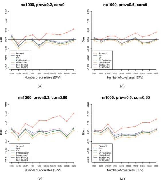
Figure 2: Bias associated to each correction method according to the number of covariates included in
the logistic regression model (p∈ {1,2, . . . ,10}). The results shown are for a sample size of n=1000and
different prevalences and correlations:(a)prev=0.2andγ=0,(b)prev=0.5andγ=0,(c)prev=0.2
andγ=0.60, and(d)prev=0.5andγ=0.60.
of 0.60 (γ=0.60) and different sample sizes (n∈ {500,1000,2000}). Note that for a sample size ofn=500 the bias of 10-fold cross-validation with and without replication and the leave-one-out cross-validation is very large, but the bias decreases as the sample size increases. Thus, with a low prevalence, larger sample sizes are required for those methods to perform well.
Figure 2 shows also the bias associated to each method, but for other parameter specifications. In particular, we present the results for a sample size of n =1000, but different prevalences and correlations. Figure 2(a) depicts the bias forn=1000,
prev=0.2 and γ=0, Figure 2(b) for n=1000, prev=0.5 and γ=0, Figure 2(c) forn=1000, prev=0.5 andγ=0.60, and Figure 2(d) forn=1000, prev=0.5 and γ=0.60. These results corroborate that the bias of the apparent AUC increases as the correlation increases and/or the prevalence decreases. In all cases, leave-one-out cross-validation is the method presenting the most pessimistic behaviour (negative bias), and, as noted before, in terms of bias, split-sample validation seems to perform similarly to 10-fold cross-validation (with and without replication) and bootstrap (withB=100 andB=500). These results also show that, on average, the corrected AUCs provided by bootstrap are larger than those provided by 10-fold cross-validation (the difference between the corrected AUCs and the out-of-sample AUC is larger), and this pattern is maintained across all specifications.
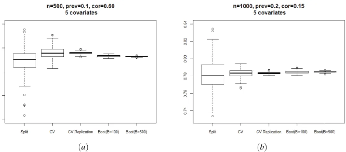
To finish with the presentation of results we show in Figure 3 the variability of the es-timated corrected AUCs when the methods were applied to 500 different random splits or resamples of a particular sample. Recall that for these results we considered the most extreme parameter specification (n =500, prev=0.1, γ=0.60) and an inter-mediate one (n=1000, prev=0.2, γ=0.15), both including 5 covariates. For both situations, it is remarkable the large variability of the split-sample validation and the 10-fold cross-validation without replication, with the other three methods (i.e., 10-fold cross-validation with replication and, bootstrap withB=100 andB=500 resamples), presenting a rather low variability (note that the scale of they-axes is different in both graphics). These results emphasise the above-discussed conclusions.
(a) (b)
Figure 3: Box-plot of the estimated corrected AUCs by means of the different correction methods when applied to 500 different splits or resamples of the same sample. This figure illustrates the variability of the
different correction methods.(a)Most extreme parameter specification (n=500, prev=0.1,γ=0.60, 5
covariates). (b)Intermediate specification (n=1000, prev=0.2,γ=0.15, 5 covariates). Note that the
4. Discussion
In this work we compared the behaviour of different methods when correcting for the optimism of the apparent AUC in logistic regression models. A large simulation study was conducted in which different scenarios were considered regarding the number of covariates, sample size, prevalence and correlation among covariates. The predictor variables were simulated following a multivariate normal distribution in such a way that the theoretical logistic regression model is known. We now summarise the main conclusions that we have drawn throughout the study.
If enough data are available, all methods seem to properly correct for the optimism of the apparent AUC, except for the leave-one-out cross-validation, which gives the most pessimistic results. Moreover, in terms of bias the behaviour of all remaining correction methods is similar (there is not a clear method that performs the best) and the bias is, in general, low. In contrast, the problems appear when the available data is insufficient and/or imbalanced. For example, when working with a low prevalence and correlated covariates, larger sample sizes will be needed to ensure a good performance of the optimism correction methods.
The results of the simulation study suggest the use of eitherk-fold cross-validation with replication or bootstrap (we note that, for cross-validation, we only examined the case ofk=10 number of folds). In particular, in the most extreme cases, the bootstrap method should be used according to these results. Even thoughk-fold cross-validation with replication and bootstrap are the most computationally demanding methods, for the sample sizes considered in this study, the computing time was affordable (in general, less than 10 seconds).
The results obtained in this work are in line with those obtained in previous studies (Austin and Steyerberg, 2017; Airola et al., 2011; Steyerberg et al., 2001; Smith et al., 2014). Nevertheless, we have also observed some differences.
On the one hand, we should note the differences in the results of the split-sample validation. In previous studies, split-sample has given pessimistic results. In contrast, in this study, the bias of the estimated AUC corrected by split-sample is very low. The reason is the following. Some researchers have claimed that despite using split-sample for the validation of the model, the final model should be based on the full sample (see, e.g., Harrell et al., 1996; Steyerberg et al., 2001). For this reason, in previous studies, the AUC corrected with split-sample was compared to the “true” out-of-sample AUC of the full model (see, e.g., Austin and Steyerberg, 2017). Nevertheless, at least in our experience, in practice, the model reported when split-sample validation is used is, in general, the one developed in the derivation sample and not derived using the whole sample (see, e.g., Quintana et al., 2014; Wada et al., 2017). Thus, in this study, we compared the AUC corrected by split-sample validation to the “true” out-of-sample AUC of the model fitted to the derivation sample. Our results suggest that, in terms of the bias, split-sample validation properly corrects the apparent AUC of the model fitted to the derivation sample. However, similarly to the results obtained in the
above-mentioned studies, the variability of the split-sample validation is very large compared to the other available methods. Furthermore, as only half of the data is used to derive the model, model’s performance is in general worse than when the full sample is used, and the “true” AUC of the model fitted to the derivation sample is also lower, unless enough data is available. We conclude that we do not recommend the use of the split-sample validation, because of its large variability and the worse performance of the final model. On the other hand, for the same EPV values, very different results were obtained in this study. For instance, for an EPV=10, for some parameter specifications the optimism of the apparent AUC was successfully corrected, but for other parameter specifications, the methods presented some bias. Thus, in addition to the EPV, the factors that were analysed in this study (the number of covariates in the model, the available sample size, the prevalence of the disease and the correlation among covariates) should also be regarded when correcting for the optimism of the apparent AUC.
We would like to conclude commenting on the limitations of our study. In the first place, we only studied the impact from 1 to 10 covariates in the model. In our daily practice, it is not common to fit models with more than 10 covariates. Nevertheless, in some cases, it could be interesting to study the impact of a larger number of covariates in the behaviour of different correction methods (see, e.g., Airola et al., 2011). Secondly, in our simulation study, we only considered the case of multivariate normally distributed covariates. However, the results we obtained are in concordance with a similar simula-tion study we conducted based on categorical covariates (results not shown), as well as with the results other authors obtained in previous studies (Austin and Steyerberg, 2017; Steyerberg et al., 2001; Smith et al., 2014). Also, for cross-validation we only examined the case ofk=10. For small sample sizes and unbalanced data, this value may be too large as it may yield into folds with very few events, thus affecting the behaviour of the method. Further research is therefore guaranteed to study the impact of the number of folds. Another limitation of this study is that we did not focus on important aspects in the development of a prediction model, such as variable selection and model derivation, but we went directly to the evaluation of the performance (and its optimism correction) of a “pre-defined” model. Moreover, as noted in the introduction, we focused on the discrimination of the model (measured by the AUC) rather than on its calibration (e.g. goodness-of-fit), which should also be considered when developing prediction models. An interesting area of research would be the study of the behaviour of the methods con-sidered in this work when applied to measures of calibration. Finally, we did not study the behaviour of the leave-pair-out cross-validation, which has shown good behaviour in previous studies (see, e.g., Airola et al., 2011; Smith et al., 2014). We focused the simulation study on the most commonly used correction methods in the literature.
A Appendix
Let us assume that the vector of p covariates XXX is distributed according to a multi-variate normal distribution in both healthy and diseased populations. That is to say,
X
XXD0 ≡XXX|D=0∼N(µµµD0,ΣΣΣ) andXXXD1 ≡XXX|D =1 ∼N(µµµD1,ΣΣΣ), where the variance-covariance matrix ΣΣΣ is assumed to be the same for both distributions. Given that ΣΣΣ
is a symmetric matrix, it can be shown thatΣΣΣ−1= 1
|ΣΣΣ|AAA, where|ΣΣΣ|denotes the determi-nant ofΣΣΣandAAAis the adjoint matrix ofΣΣΣ. Under these assumptions, it is easy to show that the logistic regression model (see eqn. (1)) holds and that the true values of the regression coefficients are
β0=ln P(D=1) P(D=0) − 1 2|ΣΣΣ| Pp k=1 Pp j=1Ajk(µD1jµD1k−µD0jµD0k), βk= 1 |ΣΣΣ| Pp j=1Ajk(µD1j−µD0j), (k=1, . . . ,p). Funding
This study was partially supported by grants Severo Ochoa Program SEV-2013-0323, Basque Government BERC Program 2018-2021, IT620-13 from the Departamento de Educaci´on, Pol´ıtica Ling ¨u´ıstica y Cultura del Gobierno Vasco and through project MTM2017-82379-R funded by (AEI/FEDER, UE) and acronym “AFTERAM”, and projects MTM2014-55966-P and MTM2016-74931-P from the Ministerio de Econom´ıa y Competitividad and FEDER. Amaia Iparragirre was partially supported by an Inter-ship Position at BCAM - Basque Centre for Applied Mathematics.
Conflict of interest
The authors declare that there are no conflicts of interest.
References
Airola, A., Pahikkala, T., Waegeman, W., De Baets, B., and Salakoski, T. (2011). An experimental com-parison of cross-validation techniques for estimating the area under the ROC curve.Computational Statistics & Data Analysis, 55, 1828–1844.
Austin, P.C. and Steyerberg, E.W. (2017). Events per variable (EPV) and the relative performance of dif-ferent strategies for estimating the out-of-sample validity of logistic regression models. Statistical Methods in Medical Research, 26, 796–808.
Bamber, D. (1975). The area above the ordinal dominance graph and the area below the receiver operating characteristic graph.Journal of Mathematical Psychology, 12, 387–415.
Bradley, A.P. (1997). The use of the area under the ROC curve in the evaluation of machine learning algorithms.Pattern Recognition, 30, 1145–1159.
Copas, J. and Corbett, P. (2002). Overestimation of the receiver operating characteristic curve for logistic regression.Biometrika, 89, 315–331.
Efron, B. (1983). Estimating the error rate of a prediction rule: improvement on cross-validation.Journal of the American Statistical Association, 78, 316–331.
Efron, B. (1986). How biased is the apparent error rate of a prediction rule? Journal of the American Statistical Association, 81, 461–470.
Efron, B. and Tibshirani, R.J. (1993).An Introduction to the Bootstrap. New York: Chapman & Hall/CRC. Garcia-Gutierrez, S., Quintana, J.M., Ant´on-Ladislao, A., Gallardo, M.S., Pulido, E., Rilo, I., Zubillaga, E., Morillas, M., Onaindia, J.J., Murga, N., et al. (2017). Creation and validation of the acute heart failure risk score: AHFRS.Internal and Emergency Medicine, 12, 1197–1206.
Hanley, J.A. and McNeil, B.J. (1982). The meaning and use of the area under a receiver operating charac-teristic (ROC) curve.Radiology, 143, 29–36.
Harrell, F.E. (2001). Regression Modeling Strategies: With Applications to Linear Models, Logistic and Ordinal Regression, and Survival Analysis. New York: Springer.
Harrell, F.E., Lee, K.L. and Mark, D.B. (1996). Multivariable prognostic models: issues in developing models, evaluating assumptions and adequacy, and measuring and reducing errors. Statistics in Medicine, 15, 361–387.
Hastie, T., Tibshirani, R. and Friedman, J. (2001).The Elements of Statistical Learning. Springer Series in Statistics. Springer New York Inc., New York, NY, USA.
Hosmer, D.W. and Lemeshow, S. (2000).Applied Logistic Regression. New York, N.Y.: Wiley.
Lachenbruch, P.A. and Mickey, M.R. (1968). Estimation of error rates in discriminant analysis. Techno-metrics, 10, 1–11.
McCullagh, P. and Nelder, J.A. (1989). Generalized Linear Models, 2nd ed. London: Chapman & Hal-l/CRC.
Parker, B.J., G¨unter, S. and Bedo, J. (2007). Stratification bias in low signal microarray studies. BMC Bioinformatics, 8, 326.
Pepe, M. (2003). The Statistical Evaluation of Medical Tests for Classification and Prediction. Oxford Statistical Science Series. Oxford University Press.
Picard, R.R. and Berk, K.N. (1990). Data splitting.The American Statistician, 44, 140–147.
Quintana, J., Esteban, C., Unzurrunzaga, A., Garcia-Gutierrez, S., Gonzalez, N., Lafuente, I., Bare, M., de Larrea, N.F., Vidal, S., et al. (2014). Prognostic severity scores for patients with COPD exac-erbations attending emergency departments. The International Journal of Tuberculosis and Lung Disease, 18, 1415–1420.
Smith, G. C.S., Seaman, S.R., Wood, A.M., Royston, P. and White, I.R. (2014). Correcting for optimistic prediction in small data sets.American Journal of Epidemiology, 180, 318–324.
Snee, R.D. (1977). Validation of regression models: methods and examples.Technometrics, 19, 415–428. Steyerberg, E. (2009).Clinical Prediction Models: A Practical Approach to Development, Validation, and
Updating. Springer Science & Business Media.
Steyerberg, E.W., Bleeker, S.E., Moll, H.A., Grobbee, D.E. and Moons, K.G. (2003). Internal and external validation of predictive models: a simulation study of bias and precision in small samples.Journal of Clinical Epidemiology, 56, 441–447.
Steyerberg, E.W., Harrell, F.E., Borsboom, G.J., Eijkemans, M., Vergouwe, Y. and Habbema, J.F. (2001). Internal validation of predictive models.Journal of Clinical Epidemiology, 54, 774–781.
Stone, M. (1974). Cross-validatory choice and assessment of statistical predictions. Journal of the Royal Statistical Society. Series B (Methodological), 36, 111–147.
van Smeden, M., Moons, K.G., de Groot, J.A., Collins, G.S., Altman, D.G., Eijkemans, M.J. and Reitsma, J.B. (2018). Sample size for binary logistic prediction models: Beyond events per variable criteria. Statistical Methods in Medical Research, in press.
Wada, T., Yasunaga, H., Yamana, H., Matsui, H., Fushimi, K. and Morimura, N. (2017). Development and validation of an ICD-10-based disability predictive index for patients admitted to hospitals with trauma.Injury, in press.
Wishart, G., Bajdik, C., Dicks, E., Provenzano, E., Schmidt, M., Sherman, M., Greenberg, D., Green, A., Gelmon, K., Kosma, V., et al. (2012). PREDICT Plus: development and validation of a prognostic model for early breast cancer that includes HER2.British Journal of Cancer, 107, 800–807.