Efficient Estimation in Semiparametric
GARCH Models
FEIKE
C. DROST AND
CHRIS
A.J. KLAASSEN
∗Tilburg University and University of Amsterdam
Abstract
It is well-known that financial data sets exhibit conditional heteroskedasticity. GARCH type models are often used to model this phenomenon. Since the distribution of the rescaled innovations is generally far from a normal distribution, a semiparametric approach is advisable. Several publications observed that adaptive estimation of the Euclidean parameters is not possible in the usual parametrization when the distribution of the rescaled innovations is the unknown nuisance parameter. However, there exists a reparametrization such that the efficient score functions in the parametric model of the autoregression parameters are orthogonal to the tangent space generated by the nuisance parameter, thus suggesting that adaptive estimation of the autoregression parameters is possible. Indeed, we construct adaptive and hence efficient estimators in a general GARCH in mean type context including integrated GARCH models.
Our analysis is based on a general LAN Theorem for time-series models, published elsewhere. In contrast to recent literature about ARCH models we do not need any moment condition.
Keywords: LAN in time-series, semiparametrics, adaptivity, (integrated) GARCH (in mean).
1
Introduction.
It is a well established empirical fact in financial economics that time-series like exchange rates and stock prices exhibit conditional heteroskedasticity. Big shocks are clustered together. The original paper of Engle (1982) proposes the ARCH model to incorporate conditional het-eroskedasticity in econometric modeling of financial data sets. Bollerslev (1986) introduces the GARCH model as a generalization of ARCH. This facilitates a parsimonious parametrization which is particularly useful when shocks are important for a longer period (the idea corresponds ∗Department of Econometrics, Tilburg University, P.O. Box 90153, 5000 LE Tilburg, The Netherlands and
Department of Mathematics, University of Amsterdam, Plantage Muidergracht 24, 1018 TV Amsterdam, The Netherlands. The first author is research fellow of the Royal Netherlands Academy of Arts and Sciences (K.N.A.W.). Part of this research was done by the second author at the Euler International Mathematical Institute, St. Petersburg. The authors gratefully acknowledge the helpful comments of Bas Werker, the editor Helmut L¨utkepohl, and three anonymous referees.
to the generalization of AR to ARMA models). Several variations and extensions have been proposed in the literature. Nelson (1991) proposes the exponential GARCH model to capture the fact that the stock market is smoother in upward directions than in the opposite case (because of the leverage effect). Gourieroux and Monfort (1992) suggest a nonparametric approach. They do not restrict attention to conditional variances that depend only upon past squared observations, but they try to estimate the functional form of the conditional heteroskedastic variance from the data. Another important extension is the GARCH-M type model [cf. Engle, Lilien, and Robins (1987)]. According to the Capital Asset Pricing Model one expects higher returns due to risk premia if the asset is more risky. To model this phenomenon the conditional variance is also included in the mean equation. Lots of applications have shown the strength of the GARCH type of modeling. In this paper we do not refer to original application papers but we want to draw attention to the monograph of Diebold (1988) and the survey paper of Bollerslev, Chou, and Kroner (1992).
Despite the success of the GARCH history there are several topics that require attention. In this paper we consider the distributional assumptions on the rescaled innovations. The original formulations of GARCH type models assume that these residuals are standard normal. Diebold (1988), however, shows that this assumption is often violated in empirical examples. Typically, the innovations have fat-tailed distributions and they are also non-symmetric in several applications. Drost and Werker (1995) provide an explanation for high kurtosis if the observations arise from a GARCH data generating process in continuous time [see also Drost and Nijman (1993) and Nelson (1990a)]. Diebold (1988) suggests that the errors will be ‘more normal’ if the process is more and more aggregated. Despite the observed non-normality of the error structure Weiss (1986) and Lee and Hansen (1994) have shown that Quasi Maxi-mum Likelihood Estimation (QMLE), based upon the false assumption of normality, yields
√
n-consistent estimators, see also Lumsdaine (1989). However, the efficiency loss may be considerable. Therefore, several authors try to avoid efficiency loss, allowing the error structure to belong to some flexible parametric family of distributions. Studentt-distributions are very popular, cf., e.g., Baillie and Bollerslev (1989). As a drawback of the introduction of such parametric models of the innovation distribution we mention that the results of Weiss (1986) and Lee and Hansen (1994) do not carry over to general error distributions. While QMLE based upon the normal distribution yields√n-consistent estimators, QMLE based upon other distributions (e.g., the student distributions) generally even fails to be consistent if the true distribution is different.
In the approaches mentioned above, the stochastic error structure is still described by some finite dimensional statistical model. To avoid the introduction of a wrong parametric family of innovation distributions leading to inconsistent estimators and to be more flexible, a semiparametric approach is to be preferred. We want to estimate the conditional heteroskedastic character of the GARCH process but we do not want to restrict the class of error distributions too much. Apart from some regularity conditions we will assume the distribution of the innovations to be completely unknown. In passing we will consider the case of symmetrically distributed innovations. At first sight, these types of estimation problems seem to be much harder than the corresponding parametric ones and one would expect that optimal semiparametric estimators are less precise asymptotically than optimal parametric estimators. For lots of interesting econometric models this presumption turns out to be too pessimistic. Adaptive estimation is often possible. Adaptive estimation is just a special instance of semiparametric efficient
estimation. Just as in parametric models, in semiparametric models an efficient estimator is an asymptotically normal estimator with minimal variance. If this minimal variance is the same as when the error distribution is known, one calls the efficient estimator adaptive since it adapts, so to say, to the underlying error distribution. Typically, an estimator based on a (wrongly) specified error distribution is not efficient in the semiparametric sense. For i.i.d. observations a lot of adaptive and semiparametric results are available [cf., e.g., Bickel, Klaassen, Ritov, and Wellner (1993) [BKRW(1993) from now on] and the survey papers of Robinson (1988) and Newey (1990)]. Rigorous results are sparse in a time-series context. ARMA models are considered in detail by Kreiss (1987a,b). Some results for GARCH are obtained in Engle and Gonz´alez-Rivera (1991) and Steigerwald (1992) [see also P¨otscher (1995) and Steigerwald (1995)]. Linton (1993) discusses the semiparametric properties of ARCH models in more detail. However, these papers impose rather high moment conditions. The parameter estimates obtained in empirical work generally fail these moment conditions and, therefore, the scope for application seems to be limited.
In Drost, Klaassen, and Werker (1994b) [henceforth DKW(1994b)] a general LAN Theorem for time-series models is presented together with conditions guaranteeing the existence of efficient estimators. We will apply these results to GARCH type models, including, e.g., I-GARCH and GARCH-M, thus avoiding severe moment conditions. We do not need the existence of moments neither of the rescaled innovations in the GARCH model (admitting for example Cauchy errors) nor of the observations (as is clear from the inclusion of integrated GARCH models). Since we only assume the existence of a stationary solution of the GARCH equations, our approach captures the models commonly used. A general LAN Theorem for time-series models is also contained in Theorem 13, Section 4, of Jeganathan (1988). Based hereon is his Theorem 17, Section 4, which yields adaptive estimators for ARMA-type location models. However, this result is not directly applicable to GARCH scale models and, moreover, it heavily leans on symmetry of the innovations.
To keep notation simple we restrict attention to the popular and most commonly used GARCH(1,1) type models. This preserves the essential difficulty of GARCH (with respect to ARCH) since both the AR and the MA part are present in the conditional variance equation. All past observations show up (at an exponentially decaying rate). The statement of our theorem with respect to GARCH(1,1) is easily generalized to the general case of GARCH(p,q).
The first semiparametric results in a GARCH context were only partially successful. Engle and Gonz´alez-Rivera (1991) state “Monte Carlo evidence suggest that this semiparametric method [i.e. the discrete maximum penalized likelihood estimation technique of Tapia and Thompson (1978)] can improve the efficiency of the parameter estimates up to 50% over QMLE, but it does not seem to capture the total potential gain in efficiency. In this sense we say that the estimator is not adaptive in the class of densities with mean 0 and variance 1; that is, the estimator is not fully efficient, and it does not achieve the Cram´er-Rao lower bound. The information matrix is not block-diagonal between the parameters of interest (the ones in the mean and in the variance equation) and the nuisance parameters (the knots of the density). If we choose the parametric form of the model with a conditional parametric density defined by a shape parameter, this one being part of the parameters to estimate, we can show easily that the expectation of the cross-partial derivatives of the log-likelihood function respects the parameter of interest and the shape parameter is different from 0. In other words, the estimation of the shape parameter affects the efficiency of the estimates of the parameters of interest”
(pp. 355–356). These statements imply that the finite dimensional parameter describing the GARCH model (with the standardized error distribution as nuisance parameter) is not adaptively estimable. This is not surprising since the classical GARCH formulation contains a scale parameter, and in most models the variance is not adaptively estimable. Therefore the scale parameter is often included into the (infinite dimensional) nuisance parameter. For the GARCH model this procedure does not work: the scores w.r.t. the remaining autoregression parameters are still not orthogonal to the tangent space. Hence, complete adaptive estimation of the conditional heteroskedastic character is not possible in GARCH models. This explains the efficiency loss observed by Engle and Gonz´alez-Rivera (1991). However, calculation of the scores w.r.t. the parameters of the GARCH model shows that there are several orthogonality relations between the score space and the tangent space generated by the unknown shape. Linton (1993) and Drost, Klaassen, and Werker (1994a) [henceforth DKW(1994a)] obtain along different lines a reparametrization of the ARCH and GARCH model respectively such that the autoregression parameters are adaptively estimable and the location-scale parameters generate the most difficult one-dimensional subproblems. So, knowledge of the shape of the error distribution does not help to construct better estimators of the conditional heteroskedastic character of the GARCH process. This resembles the regression model with unknown location
µ ∈ R, regression parameterβ ∈ Rk and completely unknown error distribution, where the regression parameter β is adaptively estimable if the location parameter is included into the nuisance [see Bickel (1982)].
The paper is organized along the following lines. In Section 2 we state the LAN Theorem for a large set of GARCH(1,1) type models, including all stationary classical GARCH models such as, e.g., I-GARCH and GARCH-M. This LAN property is derived for the parametric model with the shape of the innovations known, and it implies the Convolution Theorem of H´ajek (1970) which we will state next. This Convolution Theorem yields a bound on the asymptotic performance of estimators in the parametric model and is valid, a fortiori, for the semiparametric model as well. Section 3 is devoted to the construction of an estimator of the autoregression parameters on the assumption that the shape of the innovations is unknown, i.e. within the semiparametric model. This estimator happens to attain the bound from the parametric Convolution Theorem and therefore is asymptotically efficient in the parametric model and hence in the semiparametric model, since it does not use knowledge about the shape of the innovations. Such an estimator, which attains the parametric bound in a semiparametric model, is called adaptive. The proofs of these results are based on DKW(1994b) and most of them are given in the Appendix.
A small simulation study is presented in Section 4. It turns out that the suggested optimal estimator performs as expected: the estimator performs better than QMLE and the difference with MLE (if the error distribution is known) becomes negligible when the sample size is growing large. The empirical illustration in this section shows that the efficiency loss by using QMLE may be considerable. Some conclusions are drawn in Section 5.
2
LAN and Convolution Theorem.
We consider a generalization of the reparametrized GARCH(p, q) model as given in Lin-ton (1993), withp= 0, and motivated by adaptation arguments in DKW(1994a). For notational
simplicity, we takep= q = 1. In this manner the essential difficulty of an infinite number of lags is retained. To obtain the corresponding results for the general case (withp, q ∈INfixed) a careful replacement of coefficients by vectors suffices.
Let µ ∈ IR, σ > 0, α > 0, and β > 0 be parameters and let {εt : t ∈ Z} be an i.i.d.
sequence of innovation errors with location zero, scale one, and densityg. Putξt = µ+σεt
and note thatξtis a random variable with locationµ, scaleσ, and densityσ−1g({·−µ}/σ). We
introduce the following convention: random variables, likeεand ξ, denote a typical element of the corresponding sequences{εt:t ∈Z}and{ξt:t ∈Z}.
Consider the model with observations
yt=h 1/2 t ξt =µh 1/2 t +σh 1/2 t εt, (2.1)
where the unobservable heteroskedasticity factorshtdepend on the past via
ht= 1 +βht−1+αyt2−1 = 1 +ht−1(β+αξt2−1). (2.2) Observe that the Euclidean parameterθ = (α, β, µ, σ)0is identifiable. Throughout we assume that equation (2.2) admits a stationary solution {ht : t ∈ Z}. A necessary and sufficient
condition is given by [Nelson (1990b), Theorem 2] ASSUMPTIONA
Eln{β+αξ2}<0. (2.3)
Our semiparametric analysis treats the densityg as an infinite dimensional nuisance parameter and includes all strictly stationary GARCH models of type (2.1)–(2.2). These equations contain, e.g., the classical Engle (1982)-Bollerslev (1986) GARCH model with a different parametrization and with finite second moments (β+ασ2 <1andµ= 0), and the I-GARCH model of Engle and Bollerslev (1986) (β+ασ2 = 1and µ = 0). Furthermore, our model resembles the GARCH-M model of Engle, Lilien, and Robins (1987). In the mean equation (2.1) we have included the conditional standard deviation of yt while Engle, Lilien, and
Robins (1987) include a kind of conditional variance. More precisely stated, their model is given by zt = δht+yt and µ = 0, i.e., zt = δht +σh1t/2εt. Inserting µ = 0 in (2.1) or
µ = δ = 0 in the GARCH-M model yields the classical GARCH model. Generally, risk aversion is stronger pronounced in the original GARCH-M model than in our formulation.
Suppose that we observey1, . . . , yn, and some starting valueh01initializing (2.2). It is not needed thath01arises from the stationary solution of (2.2). We are considering estimation of
θ, based onh01, y1, . . . , yn, in the presence of the infinite dimensional nuisance parameterg.
However, in this section we will fix the nuisance parameterg and in the resulting parametric model we will derive a bound on the asymptotic performance of regular estimators of θ, a so-called Convolution Theorem. To that end we choose local submodels and we will study estimation ofθlocally asymptotically. The above mentioned Convolution Theorem holds once the log-likelihood ratios of the observed random variables are locally asymptotically normal (LAN).
Observe that the model with the autoregression parametersαandβ fixed too, corresponds to the location-scale model for i.i.d. random variables since the information provided by the observationsh01, y1, . . . , ynis equal to the information contained in the i.i.d. random variables
ξ1, . . . , ξn. Consequently, the location-scale model is a parametric submodel of our
time-series model and it makes sense to assume that this submodel is regular, i.e. [see H´ajek and ˇ
Sid´ak (1967)]
ASSUMPTIONB The distribution ofεpossesses an absolutely continuous Lebesgue density
g with derivativeg0and finite Fisher information for location
Il(g) =
Z
{g0/g}2g(ε)dε (2.4)
and for scale
Is(g) =
Z
{1 +εg0/g(ε)}2g(ε)dε. (2.5) Moreover, the random variableεhas location zero and scale one.
To be able to derive an asymptotic lower bound we have to rely on semiparametric methods as presented in, e.g., BKRW(1993) and DKW(1994a,b). So we fixθ atθ0 = (α0, β0, µ0, σ0)0 and choose local parametrizationsθn = (αn, βn, µn, σn)0 andθ˜n = ( ˜αn,β˜n,µ˜n,σ˜n)0 such that
|θn−θ0|=O(n−1/2),|θ˜n−θ0|=O(n−1/2), and even
λn=
√
n(˜θn−θn)→λ, asn→ ∞. (2.6)
In the remainder expectations, convergences, etc. are implicitly taken underθn andg (unless
otherwise indicated).
To obtain a uniform LAN Theorem we consider the log-likelihood ratioΛnofh01, y1, . . . , yn
forθ˜nwith respect toθnunderθn(andg fixed). Observe that the residuals and the conditional
variances up to timetcan be recursively calculated fromθand the observationsh01, y1, . . . , yt:
withh1(θ) =h01, obtain fort= 1,2, . . .
ξt(θ) = yt/ht1/2(θ), (2.7)
εt(θ) = {ξt(θ)−µ}/σ, (2.8)
ht+1(θ) = 1 +βht(θ) +αyt2. (2.9)
Conditionally onh01the density ofy1, . . . , ynunderθnis n Y t=1 σn−1h−nt1/2g(σn−1{h−nt1/2yt−µn}) = n Y t=1 σn−1h−nt1/2g({ξnt−µn}/σn) = n Y t=1 σn−1h−nt1/2g(εnt), wherehnt =ht(θn),ξnt =ξt(θn), andεnt =εt(θn).
To enhance the interpretation of this formula and to stress the link between the present time-series model and the i.i.d. location-scale model we introduce the notation˜hnt =ht(˜θn),
l{µ, σ}(x) = logg({x−µ}/σ)−logσ, Mnt Snt ! =n1/2σn−1hnt−1/2 µ˜n˜h 1/2 nt −µnh 1/2 nt ˜ σn˜h1nt/2−σnh1nt/2 ! , (2.10)
andε˜nt =εt(˜θn). WithΛsnthe log-likelihood ratio forh01, the log-likelihood ratioΛn may be written as Λn = log ( n Y t=1 ˜ σn−1˜hnt−1/2g(˜εnt)/ n Y t=1 σn−1h−nt1/2g(εnt) ) + Λsn = n X t=1 n l{(µn, σn) +σnn−1/2(Mnt, Snt)}(ξnt)−l{µn, σn}(ξnt) o + Λsn = n X t=1 n l{(0,1) +n−1/2(Mnt, Snt)}(εnt)−l{0,1}(εnt) o + Λsn. (2.11) This expression resembles the log-likelihood ratio statistic for the i.i.d. location-scale model but here the deviationsMntandSntare random. In the i.i.d. case the LAN Theorem is obtained
with deterministic sequences. We will apply the results of DKW(1994b) which allow for such random sequences.
To get rid of the starting condition in the log-likelihood ratio statistic we will use the following regularity condition [compare assumption (A.3) of Kreiss (1987a) and Assumption A of DKW(1994b)].
ASSUMPTIONC The densityg¯θ of the initial valueh01satisfies, underθn,
Λsn= log{g¯θ˜n/g¯θn(h01)}
P
→0, asn→ ∞. (2.12)
To make an appropriate expansion ofΛnit will be handy to introduce the notationl˙ntfor the
four-dimensional conditional score at timet. To be more precise, denote the two-dimensional vector derivative of the conditional variance by
Ht(θ) = ∂ ∂(α, β)ht(θ) =βHt−1(θ) + yt2−1 ht−1(θ) ! , (2.13)
withH1(θ) = 02. Define the(4×2)-derivative matrixWt(θ)[motivated by differentiation of
(Mnt, Snt)with respect toθ˜natθn] by Wt(θ) =σ−1 1 2h −1 t (θ)Ht(θ)(µ, σ) I2 ! , (2.14)
denote the location-scale score by (withl0 =g0/g)
ψt(θ) =− l0(εt(θ)) 1 +εt(θ)l0(εt(θ)) ! , (2.15) and put ˙ lt(θ) =Wt(θ)ψt(θ).
Then, the conditional score at timet may be denoted byl˙nt = ˙lt(θn). Observe thatl˙is just
the heuristic score. An expansion of (2.11) shows that the log-likelihood ratio Λn may be
alternatively written as Λn=λ0n−1/2 n X t=1 ˙ lnt− 1 2n −1 n X t=1 {λ0l˙nt}2+Rn. (2.16)
The LAN result for the parametric version of model (2.1)–(2.2) is stated in the following theorem. The proof is deferred to Appendix A.
Theorem 2.1 (LAN) Suppose that Assumptions A–C are satisfied. Then the local log-likelihood ratio statisticΛn, as defined by (2.11) and (2.16), is asymptotically normal. More
precisely, underθn, Rn P →0, Λn D →N −1 2λ 0I(θ 0)λ, λ0I(θ0)λ , asn→ ∞, (2.17)
whereI(θ0)is the probability limit of the averaged score productsl˙ntl˙0nt.
We are now in a position to apply the Convolution Theorem of H´ajek (1970); cf. Theorem 2.3.1, p. 24, of BKRW(1993).
Theorem 2.2 (Convolution Theorem) Under the assumptions of the LAN Theorem 2.1 let {Tn :n∈IN}be a regular sequence of estimators ofq(θ), whereq : IR4 →IRkis differentiable
with total differential matrixq◦. As usual, regularity atθ =θ0means that there exists a random
k-vectorZ such that for all sequences{θn:n∈IN}, withn1/2(θn−θ0) =O(1),
n1/2{Tn−q(θn)} D
→Z, asn→ ∞, (2.18)
where the convergence is underθn. Let˜l =
◦
q(θ0)I(θ0)−1l˙(θ
0)be the efficient influence function, then, underθ0, n1/2{Tn−q(θ0)−n−1Pnt=1˜lt} n−1/2Pnt=1˜lt ! D → ∆0 Z0 ! , asn→ ∞, (2.19)
where∆0andZ0 are independent andZ0 isN(0,
◦
q(θ0)I(θ0)−1 q◦(θ
0)0). Moreover,{Tn :n∈
IN} is efficient if{Tn : n∈ IN}is asymptotically linear in the efficient influence function, i.e.
if∆0 = 0(a.s.).
As a conclusion from the Convolution Theorem we obtain that a regular estimatorθˆnofθ
satisfies, underθ0, √
n(ˆθn−θ0)
D
→∆0+Z0,
i.e. the limit distribution of θˆn is the convolution of the random vector ∆0 and a Gaussian random vector with mean zero and variance the inverse of the information matrixI(θ0). Since
∆0 adds noise to the Gaussian vector Z0, it is clear that ∆0 = 0 would be preferred. This motivates the usual terminology (as lower bound, etc.) because∆0 = 0is attainable in lots of situations.
In the remainder of this paragraph we simplify exposition by supposing that the scores given above are stationary such that we may restrict attention to just one specific element, compare DKW(1994a). In this way it is easier to comprehend the specific adaptiveness features in the GARCH model. These results are derived along the lines of Sections 2.4 and 3.4 of BKRW(1993). This expository simplification will be suppressed again in the next section when deriving a (semiparametric) efficient estimator. This optimal estimator satisfies the properties obtained in I–IV below.
In a stationary setting the Fisher information matrix defined in the LAN Theorem 2.1 simplifies to
whereIls(g)is the information matrix in the location-scale model, Ils(g) =Eψψ0 = E(l0)2 Eε(l0)2 Eε(l0)2 E(1 +εl0)2 ! .
If the location parameterµis known to be zero, as in the classical GARCH case, this formula simplifies even further to
I(θ0) =Is(g)EWsWs0, (2.20)
whereWsis the 3-dimensional subvector ofW concerning the relevant derivatives with respect
to the scale parameterσand whereIs(g) =E(1 +εl0)2is the information for scale in the i.i.d.
scale model.
I. Ifg is known and if we want to estimate the autoregression parameterν = (α, β)0
in the presence of the nuisance parameterη= (µ, σ)0then we see that the efficient influence function, as defined in the Convolution Theorem 2.2, equals
˜
l = (I2,02×2)[El˙l˙0]−1l˙= (I2,02×2)I(θ0)−1l.˙
As in Proposition 2.4.1.A and formula (2.4.3), pp. 28,30, of BKRW(1993) we may write
˜
l = [El∗1l1∗0]−1l1∗, (2.21) where the so-called efficient score functionl∗1 of νis obtained by the componen-twise projection of l˙1, the first two elements of l˙, onto the orthocomplement of
[ ˙l2], the linear span of the last two components ofl˙. Here the inner product is the covariance and the orthocomplement is taken in the linear space spanned by all components ofl˙. It is easy to verify that
l1∗= 1 2σ
−1{(H/h)−E(H/h)}(µ, σ)ψ (2.22)
and thatl1∗is orthogonal tol˙2indeed, sinceH/h=Ht/htdepends on the past only
and is independent of the present innovationεt.
II. If g is unknown and if we want to estimate ν in the presence of the nuisance parametersη andg then we obtain the same efficient influence function. To see this note that the components of l∗1 as given in (2.22) are orthogonal to every element ofL02(ε)by the independence of present (ξandε) and past (handH). By (3.4.2) and Corollary 3.4.1.A, pp. 70,72, of BKRW(1993) we obtain
I(P0 |ν, Q)≥El∗1l1∗0 (2.23) for all regular parametric submodelsQ of our semiparametric modelP, i.e. the information at P0 in estimation of ν within the parametric submodel Q equals at least the information at P0 in estimation of ν within the parametric model, studied in I, withg known. In other words, as far as estimation ofνis concerned, no parametric model Q is asymptotically more difficult to first order (contains less information) than the model from I. Consequently the semiparametric model
P itself is asymptotically to first order as difficult as the parametric model with
g known, i.e. the information matrix with respect to ν evaluated at P0 for the semiparametric modelP equals the lower bound in the parametric model withg
known (case I),
I(P0 |ν,P) =El1∗l∗10.
Once more, the efficient influence function is given by (2.21). Apparently, in-troduction of the nuisance parameterg in the presence of the Euclidean nuisance parameterηdoes not change the efficient influence function forν. Hence, estima-tion ofνis asymptotically as hard not knowingg as knowingg. One usually calls this adaptivity. Observe, however, that the presence of the nuisance parameterη
is important to derive this result. If η is known adaptive estimation of ν is not possible! The same conclusion applies ifη is included into the “big” infinite di-mensional nuisance parameterg. So, the nuisance parameterηis treated in another way than the nuisance parameterg. Since location-scale parameters are almost always present in econometric models a different treatment is not unreasonable and the usage of the protected notion “adaptivity” is legalized. However, with the comments above in mind, a more appropriate way of saying this is to call the parameterν η-adaptive, explicitly referring to the remaining nuisance parameters present in the model. [Of course, a similar remark applies to, e.g., the non-symmetric regression model as discussed in Bickel (1982), where the regression parameterβis not fully adaptively estimable. In factβisµ-adaptive.]
III. Estimation of the remaining parameterηis completely analogous to the location-scale problem for i.i.d. variables. Obtain the well-known lower bound forη in the semiparametric location-scale model. It suffices to construct a sequence of estimators {ηˆn, n ∈ IN} for η attaining this bound. Let θˆn be some initial
√
n -consistent estimator of θ, calculate ˆhnt = ht(ˆθn) by plugging in θˆn into (2.9)
and obtain the residuals ξˆnt = ξt(ˆθn) = yt/ˆh1nt/2, similarly. If one proceeds as
if the ξˆnt are i.i.d. observations from some location-scale model, one obtains a
semiparametric efficient estimator forη in our model (as is easily verified from the Convolution Theorem 2.2 by choosing an appropriate functionq). To be more explicit, we assume thatghas finite second moment and we define the location and scale parameters by standardizingg via the equationsEgε = 0,Egε2 = 1. Then
the square root of the sample variance is optimal forσ both in the symmetric and non-symmetric case. The sample mean is optimal forµif no symmetry is assumed and under the assumption of symmetry one has to use an efficient estimator for the symmetric location-problem [cf. Example 7.8.1, p. 400, of BKRW(1993)]. If one wants to avoid moment conditions onεone may define the location-scale parameter in another way, see the discussion of the M-estimator in Section 3. IV. Finally, when estimating the whole Euclidean parameter θ, the efficient score is
simply obtained from II and III. Following the arguments leading to (2.23) in II, this score function yields a lower bound indeed. Optimality of this bound follows from III by choosing the most difficult direction from the location-scale problem.
Obvious substitutions in Theorems 2.1 and 2.2 show that the conclusions above are also valid for the classical GARCH model with µ = Egξ = 0. An optimal estimator of σ in the
non-symmetric case is given then by the square root of [cf. Example 3.2.3, pp. 53–55, of BKRW(1993)] n−1 n X t=1 ˆ ξnt2 −n−1 Pn t=1ξˆnt3 Pn t=1ξˆnt2 n X t=1 ˆ ξnt.
In the symmetric case the limiting behavior of this estimator and the square root of the sample variance are the same.
3
Adaptive Estimators.
In classical parametric models the Maximum Likelihood Estimator is asymptotically efficient, typically. In semiparametric models such an estimation principle yielding efficient estimators does not exist. However, there exist methods to upgrade√n-consistent estimators to efficient ones by a Newton-Raphson technique, provided it is possible to estimate the relevant score or influence functions sufficiently accurately. In Klaassen (1987) such a method based on “sample splitting” is described for i.i.d. models. Schick (1986) uses both “sample splitting” and Le Cam’s “discretization”, again in i.i.d. models. See, e.g., Section 7.8 of BKRW(1993) for details. Schick’s (1986) method has been adapted to time-series models in Theorem 3.1 of DKW(1994b). We assume the existence of such a preliminary,√n-consistent estimator.
ASSUMPTIOND There exists a√n-consistent estimatorθˆnofθn(underθnandg).
For our GARCH model a natural candidate for such an initial estimator is the MLE based on the assumption of normality of the innovationsεt. One often calls this estimator the Quasi MLE.
Probably, this QMLE is √n-consistent under every densityg withEgε4 < ∞; this has been
shown by Weiss (1986) for ARCH models and under restrictions by Lee and Hansen (1994) for GARCH models, which are slightly different from ours, see also Lumsdaine (1989). The additional moment condition on εis needed there since a quadratic term appears in the score function of the scale parameter. To avoid moment conditions altogether, one could use, e.g., another preliminary M-estimator, instead. Letχ: IR →IR2 be a sufficiently smooth bounded function with monotonicity properties. As an example we mentionχ= (χ1, χ2)0 with
χ1(x) =
2
1 + exp{−x} −1, x∈IR,
the location score function for the logistic distribution and
χ2(x) =
Z x
0
2y exp{−y}
(1 + exp{−y})2dy−1, x∈IR. The M-estimator will solve the equations [cf. (2.7)–(2.9) and (2.13)–(2.14)]
n
X
t=1
Use of this M-estimator implies that one standardizesgat location0and scale1by the equation
Egχ(ε) = 0; in the normal case with QMLE this yields µas expectation and σ as standard
deviation.
To prove that estimation via (3.1) shows validity of Assumption D we have to prove existence of this M-estimator and its√n-consistency. It should be possible to show existence along the lines of Scholz (1971) by studying the 4 by 4 pseudo information matrix EW χχ0W0; see also Huber (1981), pages 138-139. Here we will not attempt to do this, since the situation is much more complicated than the location-scale problem studied in the literature. At the cost of some generality we suppose here that√n-consistent estimatorsαˆn andβˆnare given. The
√
n-consistency ofαˆnandβˆntogether with the contiguity obtained from the LAN Theorem 2.1
implies that we may treat the parametersα and β as given. So, we are in fact in the i.i.d. location-scale model and the M-estimators forµandσsolving the latter two equations in (3.1) are√n-consistent, see Huber (1981) and Bickel (1982). We conjecture that the proof of the more general M-estimator solving (3.1) can be given along similar lines.
Here we will focus on efficient and hence adaptive estimation of the autoregression param-etersαandβ(cf. Subsections I–IV of Section 2); alternatively, in view of (2.14), note that the score l˙nt satisfies the form discussed in Example 3.1 of DKW(1994b). In the Appendix we
verify the conditions of Theorem 3.1 in DKW(1994b), this yields the following theorem. Theorem 3.1 Under Assumptions A–D adaptive estimators ofαandβdo exist.
To describe our adaptive estimator more accurately, let θˆn = ( ˆαn,βˆn,µˆn,σˆn)0 be a
√
n -consistent estimator ofθ and compute Wt(ˆθn) via (2.13) and (2.14). Letεˆn1, . . . ,εˆnn be the
residuals computed from h1, y1, . . . , yn and θˆn using (2.8). Via a kernel estimate based on
ˆ
εn1, . . . ,εˆnnwith the logistic kernel, sayk(·), and bandwidthbnwe estimateg(·)by
ˆ gn(·) = 1 n n X t=1 1 bn k · −εˆnt bn !
and subsequently ψ(·) by ψˆn(·); here bn → 0 and nb4n → ∞. Now our estimator may be
written as ( ˆαn,βˆn)0 + (I2,02×2)( 1 n n X t=1 Wt(ˆθn) ˆψn(ˆεnt) ˆψn(ˆεnt)0Wt(ˆθn)0)−1 × 1 n n X t=1 ( Wt(ˆθn)− 1 n n X s=1 Ws(ˆθn) ) ˆ ψn(ˆεnt). (3.2)
With θˆn the QMLE this is the estimator used in the simulations of Section 4. To prove that
such estimators are adaptive we need the following two technical modifications.
• Discretization. θˆnis discretized by changing its value in(0,∞)×(0,∞)×IR×(0,∞)
into (one of) the nearest point(s) in the grid √c
n(IN×IN×Z×IN). This technical trick
enables one to considerθˆnto be non-random, and therefore independent ofεˆnt,yt, and
h1.
• Sample Splitting. The set of residualsεˆn1, . . . ,εˆnnis split into two samples, which may
estimateψ(·)by ψˆn2(·)and ψˆn(ˆεnt) in (3.2) is replaced byψˆn2(ˆεnt). Similarly for εˆnt
in the second sample, the first sample is used to estimateψ(·). In this way, again some independence is introduced artificially to make the proof work.
This approach has been adopted in DKW(1994b). It should be emphasized that both tricks are merely introduced as a technical device to make proofs work. Other approaches have also been studied in the literature. Klaassen (1987) has shown that discretization may be avoided at the cost of an extra sample splitting. Schick (1986) and Koul and Schick (1995) show that sample splitting may be avoided at the cost of some extra conditions.
4
Simulations and an Empirical Example.
To enhance the interpretation and validity of the theoretical results of the previous sections we present a small simulation experiment. Furthermore, a case study concerning some exchange rate series is given.
We simulated several GARCH(1,1) series of length n = 1000, parameters (α, β, σ) = (.3, .6,1), (.1, .8,1), and (.05, .9,1) [the parameter µ is set to zero and is not estimated to allow for a better comparison with previous simulation studies], and eight different innovation distributions: normal, a balanced mixture of two standard normals with means 2 and −2, respectively, double exponential, student distributions withν = 5,7, and9degrees of freedom, and (skew) chi-squared distributions withν = 6and 12degrees of freedom. These densities are rescaled such that they have the required zero mean and unit variance.
It is the purpose of the simulations to evaluate the moderate sample properties of the autoregression parametersαandβwhich are adaptively estimable, in principle. For each series we estimated these parameters with MLE, QMLE, and a one-step semiparametric procedure. For the latter estimation method we made two estimates: one under general assumptions on the innovation distribution and one under the extra assumption of symmetry. The theoretical results imply that there should be no difference between these two semiparametric methods if the true underlying density is symmetric indeed but small sample properties may differ. In the semiparametric part we used standardized logistic kernels with a bandwidth of h = .5. Reasonable changes of the bandwidth, say.25 ≤ h ≤ .75, or another kernel like the normal one do not alter the conclusions below.
In the first part of the simulation experiment we compared the ML estimator with the semi-parametric ones (with the MLE as initial starting value). Asymptotically both semisemi-parametric estimators should behave as well as the MLE but one may expect that the small sample prop-erties of the semiparametric estimators are worse due to the inherent problems of choosing the bandwidth. These results are not reported here but they are comparable to those given in Table 4.1, from which MLE can be compared with the semiparametric procedure with the less efficient QMLE starting value.
Of course ML estimation is not feasible in practice since the underlying distribution is not known. Therefore, we used the QMLE as starting point. Sinceµ vanishes for the situation chosen here and ασ2 +β < 1, Theorems 2 and 3 of Lee and Hansen (1994) are applicable and the QMLE is√n-consistent. This estimator has been improved by the one-step Newton method. For convenience we also report the behavior of the unfeasible MLE in Table 4.1. The
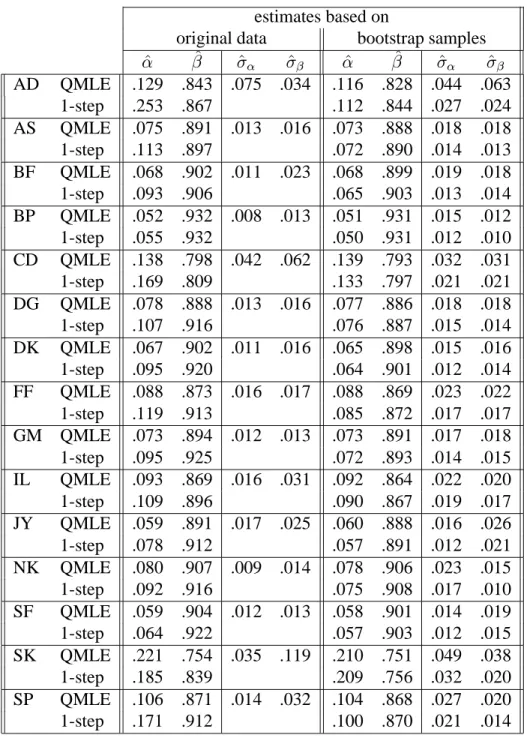
α β α β α β .300 .600 .100 .800 .050 .900 ˆ α βˆ σˆα σˆβ αˆ βˆ σˆα σˆβ αˆ βˆ σˆα σˆβ N ML=QML .298 .593 .071 .056 .099 .786 .035 .073 .047 .891 .022 .051 1-step .298 .593 .072 .057 .098 .786 .036 .074 .047 .892 .022 .050 1-step(sym) .298 .593 .072 .056 .099 .786 .036 .073 .047 .891 .022 .051 DE ML .299 .592 .080 .070 .099 .782 .038 .083 .048 .885 .023 .061 QML .303 .588 .089 .079 .100 .776 .043 .094 .048 .880 .026 .073 1-step .294 .593 .085 .074 .097 .784 .040 .087 .046 .886 .024 .067 1-step(sym) .295 .592 .083 .073 .097 .783 .039 .086 .046 .885 .024 .065 NM ML .295 .595 .058 .041 .098 .790 .029 .054 .047 .898 .018 .030 QML .295 .595 .059 .042 .097 .790 .030 .054 .046 .897 .018 .032 1-step .295 .595 .060 .043 .098 .793 .030 .056 .047 .901 .018 .032 1-step(sym) .295 .595 .059 .042 .099 .793 .030 .056 .047 .901 .018 .032 t5 ML .295 .592 .076 .067 .100 .787 .036 .071 .048 .888 .021 .054 QML .296 .586 .098 .086 .101 .777 .047 .101 .048 .879 .027 .083 1-step .284 .594 .080 .071 .094 .791 .037 .081 .044 .890 .022 .064 1-step(sym) .285 .594 .079 .070 .095 .791 .037 .081 .045 .889 .022 .063 t7 ML .296 .595 .075 .060 .100 .782 .037 .079 .047 .885 .021 .063 QML .298 .592 .086 .070 .101 .776 .042 .094 .047 .882 .024 .076 1-step .291 .597 .078 .064 .096 .784 .038 .082 .045 .886 .022 .068 1-step(sym) .292 .597 .077 .063 .097 .783 .038 .082 .045 .886 .022 .068 t9 ML .298 .592 .076 .060 .098 .783 .037 .077 .047 .887 .022 .058 QML .300 .591 .083 .066 .099 .781 .040 .085 .048 .886 .024 .064 1-step .295 .593 .079 .062 .096 .785 .038 .080 .046 .889 .022 .057 1-step(sym) .295 .593 .077 .062 .096 .784 .038 .079 .046 .889 .022 .057 χ2 6 ML .297 .596 .042 .034 .099 .796 .020 .036 .050 .899 .012 .022 QML .299 .589 .091 .073 .101 .780 .042 .096 .048 .884 .024 .072 1-step .283 .603 .062 .051 .092 .801 .030 .061 .045 .898 .017 .047 χ212 ML .298 .596 .057 .045 .099 .794 .029 .048 .048 .893 .016 .036 QML .299 .592 .084 .064 .100 .782 .041 .079 .047 .881 .023 .071 1-step .289 .598 .065 .051 .095 .796 .032 .061 .045 .891 .018 .049
Table 4.1: Comparison of MLE, QMLE, and two semiparametric one-step estimators in the GARCH(1,1) model with eight different standardized innovation distributions. Number of observationsn= 1000, true parameters(α, β) = (.3, .6),(.1, .8), and (.05, .9), respectively. The sample means of2500 independent replications and their sample standard deviations are given.
mean values of the estimates in2500replications are given together with their sample standard deviations.
To calculate the efficiency of the QMLE, observe that the asymptotic variance of the QMLE is equal to the well-known variance formula A−1BA−1, where A is the expectation under
(α, β, σ, g) of the second derivative of the pseudo log-likelihood (with a wrongly specified normal density) andB the expectation of the squared first derivative. WithWsas defined just
below (2.20), straightforward calculations show
A = 2EWsWs0,
B = (κ−1)EWsWs0,
where κ = R ε4g(ε)dε. Except for the normal distribution, the matrices A−1 and B−1 are generally not equal. Since the asymptotic variance of the QMLE is equal to the lower bound up to a constant, the asymptotic efficiency of each component of the QMLE is given by
4 (κ−1)Is(g)
= R 4
(ε2−1)2g(ε)dεR(1 +εl0(ε))2g(ε)dε ≤1.
The latter inequality follows from Cauchy-Schwarz applied to the following identity
−2 = E(ε2−1)(1 +εl0(ε)) =
Z
(ε2−1)(1 +εl0(ε))g(ε)dε.
Since the lower bound forαandβdoes not change in the semiparametric setting, this expres-sion also entails the loss in the semiparametric model and shows the (potential) gain of the semiparametric estimator (3.2).
Except for the mixture distribution we can exactly calculate the efficiency of QMLE with respect to MLE. For the standardized double exponential the relative efficiency is 45, for stan-dardized student distributions withνdegrees of freedom it is1− ν(ν12−1), and for standardized chi-squared distributions withν degrees of freedom it isνν−+64. For these heavy-tailed distribu-tions the efficiency losses of QMLE with respect to MLE show up in Table 4.1 and we see that the semiparametric methods regain most of the loss caused by the inefficient QMLE method. For light-tailed alternatives, as in the mixture case, the situation is less clear cut. There the efficiency is approximately .94 and the performance of the estimators is not much different. For the normal distribution MLE and QMLE are of course equivalent. The use of the additional symmetry information hardly improves the estimated standard deviation of the semiparametric estimator (maximal .002), just as expected from our general theory. In empirical data sets one often observes outlier type innovation distributions with high kurtoses. Therefore, it seems worthwhile to apply the semiparametric estimation programs in these situations.
We conclude this section with a simple empirical example based on daily data. We applied our estimation methods to fifteen logarithmic differenced exchange rate series for the period January 1, 1980 to April 1, 1994 (n = 3719): Austrian Schilling (AS), Australian Dollar (AD), Belgium Franc (BF), British Pound (BP), Canadian Dollar (CD), Dutch Guilder (DG), Danish Kroner (DK), French Franc (FF), German Mark (GM), Italian Lire (IL), Japanese Yen (JY), Norwegian Kroner (NK), Swiss Franc (SF), Swedish Kroner (SK), and Spanish Peseta (SP), all with respect to US Dollar. These data are taken from Datastream. To facilitate the interpretation of the autoregression parameters we have standardized the series such that the
estimates based on
original data bootstrap samples
ˆ α βˆ σˆα σˆβ αˆ βˆ σˆα σˆβ AD QMLE .129 .843 .075 .034 .116 .828 .044 .063 1-step .253 .867 .112 .844 .027 .024 AS QMLE .075 .891 .013 .016 .073 .888 .018 .018 1-step .113 .897 .072 .890 .014 .013 BF QMLE .068 .902 .011 .023 .068 .899 .019 .018 1-step .093 .906 .065 .903 .013 .014 BP QMLE .052 .932 .008 .013 .051 .931 .015 .012 1-step .055 .932 .050 .931 .012 .010 CD QMLE .138 .798 .042 .062 .139 .793 .032 .031 1-step .169 .809 .133 .797 .021 .021 DG QMLE .078 .888 .013 .016 .077 .886 .018 .018 1-step .107 .916 .076 .887 .015 .014 DK QMLE .067 .902 .011 .016 .065 .898 .015 .016 1-step .095 .920 .064 .901 .012 .014 FF QMLE .088 .873 .016 .017 .088 .869 .023 .022 1-step .119 .913 .085 .872 .017 .017 GM QMLE .073 .894 .012 .013 .073 .891 .017 .018 1-step .095 .925 .072 .893 .014 .015 IL QMLE .093 .869 .016 .031 .092 .864 .022 .020 1-step .109 .896 .090 .867 .019 .017 JY QMLE .059 .891 .017 .025 .060 .888 .016 .026 1-step .078 .912 .057 .891 .012 .021 NK QMLE .080 .907 .009 .014 .078 .906 .023 .015 1-step .092 .916 .075 .908 .017 .010 SF QMLE .059 .904 .012 .013 .058 .901 .014 .019 1-step .064 .922 .057 .903 .012 .015 SK QMLE .221 .754 .035 .119 .210 .751 .049 .038 1-step .185 .839 .209 .756 .032 .020 SP QMLE .106 .871 .014 .032 .104 .868 .027 .020 1-step .171 .912 .100 .870 .021 .014
Table 4.2: Comparison of QMLE and a semiparametric one-step estimator for several loga-rithmic differenced daily exchange rate series. Observation period January 1, 1980 to April 1, 1994 (n= 3719). The first part of the table gives the estimates based on the original data set. Estimated standard deviations are deleted for the semiparametric estimators. The sample means and sample standard deviations of 500 bootstrap replications are given in the second half of the table.
QMLE ofσ is one. In all series both the QMLE method and the semiparametric procedure estimate the persistenceασ2+βless than one (for the semiparametric estimates this cannot be inferred from Table 4.2 since the semiparametric estimate ofσ is not constrained to be one). The estimates based on the original data sets are given in the first four columns of Table 4.2. Of course we used the variance formulaA−1BA−1for the direct estimate of the standard deviation of the QMLE. As described above, the parameter estimates produced by the semiparametric procedure are not very sensitive to the choice of the bandwidth. However, it turns out that the direct variance estimates change dramatically (even for small changes of the bandwidth). Therefore, these estimates are not reliable and they have been deleted from the table.
For the simulation study above the situation was quite different since we estimated the variance of the semiparametric one-step estimators from independent parameter estimates in the replications. Here we have only one data set. Independent replications are not available. This leads to the following paradox. On the one hand one may have the imprecise QML estimate with quite large estimated standard deviations. So it may be possible that the hypotheses of integrated GARCH or no conditional heteroskedasticity cannot be rejected. On the other side one has the improved semiparametric estimate which allows for more powerful tests. But since the estimated standard deviations are unreliable one can get any answer one wants by changing the bandwidth. To avoid this paradox, we propose to use the bootstrap. I.e. simulate replications of the original data set with the estimated parameter and the estimated innovation distribution as inputs and proceed as in the case of simulations described above. Then we have several parameter estimates available from which we calculate the straightforward sample estimate of the variance. In this manner we only rely upon the parameter estimates and not on direct estimates of the variance. Hence, the variability of the variance due to different bandwidth choices is greatly reduced. Some simulation experiments show that this procedure works quite well. We apply the bootstrap procedure to our data sets and we report the sample means and sample standard deviations in the final four columns of Table 4.2. Observe that the estimated standard deviations of the semiparametric estimators of the heteroskedastic parameters are between four tenth (AD) and nine tenth (IL) of the estimated ones for the QMLE method. This implies the efficiency of the QMLE method lies approximately in the interval(.15, .80)
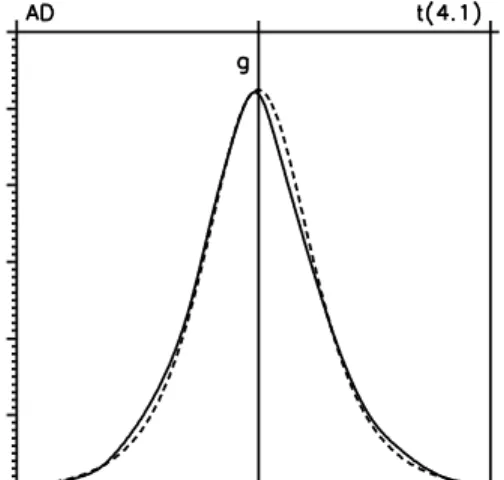
in these special examples. The efficiency gain is also supported by the plots in Figure 4.1 of the nonparametric density estimates and the corresponding score estimates which are far away from the normal density and score. Although these figures suggest some skewness of the exchange rate densities, they are close to the densities of student tν-distributions with ν
between 4.1 and 5.4. If the true underlying density would be symmetric, we expect from the simulation study that the symmetric nonparametric procedure performs slightly better in moderate samples. However, in the exchange rate applications the latter procedure yields somewhat larger standard deviations (.003 for AS and less than .002 for the others, these values are not reported here). This indicates that the true densities are not fully symmetric and hence the symmetric semiparametric approach may lead to wrong conclusions. Since the possible moderate sample loss is very small it seems to be safer to use the ordinary non-symmetric improvement.
Finally, we note that the simulation results of Table 4.1 show that all estimators, even the unfeasible MLE, tend to underestimate the heteroskedasticity parameters. This negative bias explains why in Table 4.2 on the average the bootstrap estimates are less in value than the original estimates.
0 . 0 0 . 1 0 . 2 0 . 3 0 . 4 0 . 5 0 . 6 - 3 - 2 - 1 0 1 2 3 - 3 - 2 - 1 0 1 2 3 - 3 - 2 - 1 0 1 2 3 0 . 0 0 . 1 0 . 2 0 . 3 0 . 4 0 . 5 0 . 6 - 3 - 2 - 1 0 1 2 3 - 3 - 2 - 1 0 1 2 3 - 3 - 2 - 1 0 1 2 3 0 . 0 0 . 1 0 . 2 0 . 3 0 . 4 0 . 5 0 . 6 - 3 - 2 - 1 0 1 2 3 - 3 - 2 - 1 0 1 2 3 - 3 - 2 - 1 0 1 2 3
Figure 4.1: Comparison of estimated densities and scores with tν-densities and scores for
several logarithmic differenced daily exchange rate series. Observation period January 1, 1980 to April 1, 1994 (n= 3719).
0 . 0 0 . 1 0 . 2 0 . 3 0 . 4 0 . 5 0 . 6 - 3 - 2 - 1 0 1 2 3 - 3 - 2 - 1 0 1 2 3 - 3 - 2 - 1 0 1 2 3 0 . 0 0 . 1 0 . 2 0 . 3 0 . 4 0 . 5 0 . 6 - 3 - 2 - 1 0 1 2 3 - 3 - 2 - 1 0 1 2 3 - 3 - 2 - 1 0 1 2 3 0 . 0 0 . 1 0 . 2 0 . 3 0 . 4 0 . 5 0 . 6 - 3 - 2 - 1 0 1 2 3 - 3 - 2 - 1 0 1 2 3 - 3 - 2 - 1 0 1 2 3 Figure 4.1: (CONTINUED)
0 . 0 0 . 1 0 . 2 0 . 3 0 . 4 0 . 5 0 . 6 - 3 - 2 - 1 0 1 2 3 - 3 - 2 - 1 0 1 2 3 - 3 - 2 - 1 0 1 2 3 0 . 0 0 . 1 0 . 2 0 . 3 0 . 4 0 . 5 0 . 6 - 3 - 2 - 1 0 1 2 3 - 3 - 2 - 1 0 1 2 3 - 3 - 2 - 1 0 1 2 3 0 . 0 0 . 1 0 . 2 0 . 3 0 . 4 0 . 5 0 . 6 - 3 - 2 - 1 0 1 2 3 - 3 - 2 - 1 0 1 2 3 - 3 - 2 - 1 0 1 2 3 Figure 4.1: (CONTINUED)
0 . 0 0 . 1 0 . 2 0 . 3 0 . 4 0 . 5 0 . 6 - 3 - 2 - 1 0 1 2 3 - 3 - 2 - 1 0 1 2 3 - 3 - 2 - 1 0 1 2 3 0 . 0 0 . 1 0 . 2 0 . 3 0 . 4 0 . 5 0 . 6 - 3 - 2 - 1 0 1 2 3 - 3 - 2 - 1 0 1 2 3 - 3 - 2 - 1 0 1 2 3 0 . 0 0 . 1 0 . 2 0 . 3 0 . 4 0 . 5 0 . 6 - 3 - 2 - 1 0 1 2 3 - 3 - 2 - 1 0 1 2 3 - 3 - 2 - 1 0 1 2 3 Figure 4.1: (CONTINUED)
0 . 0 0 . 1 0 . 2 0 . 3 0 . 4 0 . 5 0 . 6 - 3 - 2 - 1 0 1 2 3 - 3 - 2 - 1 0 1 2 3 - 3 - 2 - 1 0 1 2 3 0 . 0 0 . 1 0 . 2 0 . 3 0 . 4 0 . 5 0 . 6 - 3 - 2 - 1 0 1 2 3 - 3 - 2 - 1 0 1 2 3 - 3 - 2 - 1 0 1 2 3 0 . 0 0 . 1 0 . 2 0 . 3 0 . 4 0 . 5 0 . 6 - 3 - 2 - 1 0 1 2 3 - 3 - 2 - 1 0 1 2 3 - 3 - 2 - 1 0 1 2 3 Figure 4.1: (CONTINUED)
5
Conclusions.
In this paper we studied the semiparametric properties of (integrated) GARCH-M type models. In this model, adaptive estimation is not possible. This fact is completely caused by a location-scale parameter. After a suitable reparametrization of the model we showed that the estimation problem of the parameters characterizing the conditional heteroskedastic character of the process is equally difficult in cases where the innovation distribution is known or unknown, respectively. In that sense we may call these parameters still adaptively estimable. This property is derived in a general GARCH context avoiding moment conditions and including integrated GARCH models. The simulations showed that this property is not only interesting from a theoretical point of view. In moderate sample sizes withn= 1000observations, usually available in financial time-series, the semiparametric procedures work reasonably well. Most of the loss caused by the QMLE method (instead of the infeasible MLE method) is regained by the one-step estimator in case of the interesting group of heavy-tailed alternatives. Moreover, the empirical example showed that the efficiency loss caused by the QMLE method may be considerable.
It is clear from the exposition in this paper that the adaptivity results carry over to compli-cated models with time dependent mean and variance structures, e.g., ARMA with GARCH errors. The basic conditions given in DKW(1994b) do not seem to put serious restrictions on the models. However, a complete verification of the technical details may be much more demanding.
A
Appendix.
PROOF OF THELAN THEOREM2.1: Since the general GARCH model (2.1)–(2.2) is a
location-scale model in which the location-location-scale parameter only depends on the past, our model fits into the general time-series framework of DKW(1994b), especially Section 4. Therefore, it suffices to verify the conditions (2.30), (A.1), and (2.4) of DKW(1994b). In passing we also prove (3.30) of DKW(1994b) which we will need in the proof of Theorem 3.1. I.e., with the notation introduced in (2.10), (2.14), and (2.15), and Ils(g) the expectation under θ of the
productψ(θ)ψ(θ)0, we have to show, underθ0,
n−1 n X t=1 Wt(θ0)Ils(g)Wt(θ0)0 P →I(θ0)>0, n−1 n X t=1 |Wt(θ0)|21{n−1/2|W t(θ0)|>δ} P →0, (A.1) n−1 n X t=1 Wt(θ0) P →W(θ0), (A.2) n−1 n X t=1 |Wt(θn)−Wt(θ0)|2 P →0, (A.3) and, underθn, n X t=1 |n−1/2(Mnt, Snt)0−Wt(θn)0(˜θn−θn)|2 P →0, (A.4)
for some positive definite matrixI(θ0)and some random matrixW(θ0). Together with their Lemma A.1, these four relations yield the desired conclusions. We prepare the proof by deriving some helpful results.
Although Wt(θ0) is not stationary under θ0, the following proposition shows that these variables can be approximated by a stationary sequence.
Proposition A.1 Letht(θ),Ht(θ), andWt(θ)be given by (2.9), (2.13), and (2.14), respectively,
and lethst(θ),Hst(θ), andWst(θ)be their corresponding stationary solutions underθ, i.e.
hst(θ) = ∞ X j=0 j Y k=1 {β+αξ2t−k}, Hst(θ) = ∞ X i=0 βihs,t−1−i(θ) ξt2−1−i 1 ! , Wst(θ) =σ−1 1 2h −1 st (θ)Hst(θ)(µ, σ) I2 ! . Then, underθ0, n−1 n X t=1 |Wt(θ0)−Wst(θ0)|2 →0 (a.s.), asn→ ∞. (A.5)
PROOF: We adopt the convention that empty sums are equal to zero while empty products are equal to one. Iteratinght(θ)yields
ht(θ) = 1 +βht−1(θ) +αyt2−1 = 1 +ht−1(θ){β+αξ2t−1(θ)} = i−1 X j=0 j Y k=1 {β +αξt2−k(θ)}+ht−i(θ) i Y k=1 {β+αξt2−k(θ)}, 0≤i≤t−1, (A.6) and hence ht−i(θ)/ht(θ)≤ i Y k=1 {β+αξt2−k(θ)}−1, 0≤i≤t−1. (A.7)
Underθ, the calculated variablesξt(θ)simply are the true innovationsξt in (A.6) and (A.7).
For the stationary random variableshst(θ)we obtain similar relations,
hst(θ) = i−1 X j=0 j Y k=1 {β+αξt2−k}+hs,t−i(θ) i Y k=1 {β+αξt2−k}, 0≤i, hs,t−i(θ)/hst(θ) ≤ i Y k=1 {β+αξt2−k}−1, 0≤i,
and hence, underθ, we obtain
|hst(θ)ht−i(θ)−ht(θ)hs,t−i(θ)|=|hs,t−i(θ)−ht−i(θ)| i−1 X j=0 j Y k=1 {β+αξt2−k} ≤ ht(θ)|hs1(θ)−h1(θ)| t−Y1−i k=1 {β+αξ2t−i−k} = ht(θ)|hs1(θ)−h1(θ)| i Y k=1 {β+αξt2−k}−1 tY−1 k=1 {β+αξk2}, 0≤i≤t−1.
WithCsome generic constant only depending onθwe obtain, underθ, |Wt(θ)−Wst(θ)| ≤C|Ht(θ)/ht(θ)−Hst(θ)/hst(θ)| ≤ C t−2 X i=0 βi|ht−1−i(θ) ht(θ) −hs,t−1−i(θ) hst(θ) | ξt2−1−i 1 ! +C ∞ X i=t−1 βihs,t−1−i(θ) hst(θ) ξ2 t−1−i 1 ! ≤ C|hs1(θ)−h1(θ)| tY−1 k=1 {β+αξk2} t−2 X i=0 i Y k=1 β β+αξ2 t−k +C ∞ X i=t−1 i Y k=1 β β+αξ2 t−k ≤ C|hs1(θ)−h1(θ)|(t−1) tY−1 k=1 {β+αξk2}+C tY−1 k=1 β β+αξ2 k ∞ X i=−1 i Y k=0 β β+αξ2 −k .
By (2.3) the right-hand side tends to zero (a.s.), ast → ∞. Ces`aro’s Theorem completes the
proof of the proposition. 2
Intuitively it is clear that slight perturbations of the parameters yield solutions of equations (2.1) and (2.2) that are close. The following proposition makes this more precise. Just as expected from heuristic formal calculations, the leading term of˜hnt/hnt−1is a linear combination of
the components ofHnt/hnt which appears in the scorel˙nt.
Proposition A.2 Letht(θ)andHt(θ)be given by (2.9) and (2.13), respectively, and define
Qt(θ) =Ht(θ)/ht(θ) = t−2 X i=0 βi y 2 t−1−i ht−1−i(θ) ! /ht(θ) = t−2 X i=0 βiht−1−i(θ) ht(θ) ξ2 t−1−i(θ) 1 ! , Rt(θ,θ˜) =ht(˜θ)/ht(θ)−1−( ˜α−α,β˜−β)Qt(θ).
Letθnandθ˜nsatisfy the conditions just above (2.6). PutQnt =Qt(θn)andRnt =Rt(θn,θ˜n).
Then, underθn, n−1 n X t=1 |Qnt|2 =OP(1), n−1 n X t=1 |Qnt|21{n−1/2|Q nt|>δ} →0, (a.s.), asn→ ∞, (A.8) n X t=1 R2nt →0, (a.s.), asn→ ∞. (A.9)
PROOF: By equation (A.7) we obtain
Qt(θ)≤β−1 t−2 X i=0 iY+1 k=1 β β+αξ2 t−k(θ) ξ2 t−1−i(θ) 1 ! .
Fornsufficiently large, this latter relation shows that, underθn,|Qnt|may be bounded by the
product of a constant only depending onθ0and the stationary sequence
St= ∞ X i=0 i Y k=1 β0 β0+ 12α0ξ2t−k .
To prove the result concerning the remainder termRntnote that an explicit relationship for
the difference ofht(˜θ)andht(θ)is given by [compare (2.3) of Kreiss (1987a)]
ht(˜θ)−ht(θ) = t−2 X i=0 ˜ βiht−1−i(θ)( ˜α−α,β˜−β) ξ2 t−1−i(θ) 1 ! .
Hence, the remainder termRt(θ,θ˜)is given by
Rt(θ,θ˜) = t−2 X i=0 ( ˜βi−βi)ht−1−i(θ) ht(θ) ( ˜α−α,β˜−β) ξ 2 t−1−i(θ) 1 ! .
Choosec > 1such thatEcβ0/(β0 +12α0ξ21) <1. By the mean value theorem, there exists a
˜
βniin betweenβ˜nandβnsuch that, fornsufficiently large,
|β˜i n−β
i
n|=|β˜n−βn|iβ˜nii−1 ≤ |β˜n−βn|ici−1βni−1, i≥ 0.
Just as forQnt, we may boundRnt by the product of a constant timesn−1 and the stationary
sequence St∗ = ∞ X i=0 i i Y k=1 cβ0 β0+ 12α0ξ2t−k .
The proof of the proposition can be easily completed. 2
Now we are ready to prove (A.1)–(A.4). Define I(θ0) = Eθ0Ws1(θ0)Ils(g)Ws1(θ0)0 and W(θ0) = Eθ0Ws1(θ0) (the existence of these quantities can be obtained along the lines of
the proof of Proposition A.2 since |Wst(θ0)| is bounded by the product ofSt and a constant
depending onθ0, only). Obviously the relations (A.1) and (A.2) hold true ifWt(θ0)is replaced by the stationary ergodic sequenceWst(θ0). Consequently, Proposition A.1 implies the validity of these relations forWt(θ0)itself.
To prove (A.4) we will use Proposition A.2. Writingλn = (λ01n, λ02n)0 withλ1n (λ2n) the
first (latter) two components ofλn, and defining
χ(x) = n−1 + 2(√1 +x−1)/xo1{x≥−1}, we see n X t=1 |n−1/2(Mnt, Snt)0−Wt(θn)0(˜θn−θn)|2 = = σn−2n−1 n X t=1 (˜µn,˜σn)0 1 2(λ 0 1nQnt+ √ nRnt)χ(n−1/2λ01nQnt+Rnt) + 1 2 √ nRnt +n−1/2λ2n 1 2λ 0 1nQnt 2.
Together with Proposition A.2, Lemma 2.1 of DKW(1994b) [with Ynt = λ01nQnt, Xnt =
λ01nQnt+
√
nRnt, and the functionφ=χ2as above] yields (A.4).
Finally, we have to prove (A.3). Note that
and obtain contiguity ofPθn andPθ0 from (A.1) and (A.4), and Theorem 2.1 of DKW(1994b).
Then the required result is easily obtained from
Qt(˜θ)−Qt(θ) = t−2 X i=0 ( ˜βi−βi)ht−1−i(˜θ) ht(˜θ) ξ2t−1−i(˜θ) 1 ! + Qt(θ) n (θ1−θ˜1)0Qt(˜θ) +Rt(˜θ, θ) o − Pt−2 0 i=0βi h t−1−i( ˜θ) ht( ˜θ) n (θ1−θ˜1)0Qt−1−i(˜θ) +Rt−1−i(˜θ, θ) o
along the lines of the proofs of the propositions above. This completes the proofs of the
theorems in Section 2. 2
PROOF OFTHEOREM3.1: It suffices to verify the conditions of DKW(1994b). These reduce to (A.1)–(A.4) above, which are verified there, and the existence of an estimatorψˆn(·), based
onε1, . . . , εn, ofψ(·) =−(l0(·),1 +·l0(·))0, from (2.15), satisfying the consistency condition
Z
|ψˆn(x)−ψ(x)|2
g(x)dx→P 0, underg.
Indeed, such an estimator exists in view of Proposition 7.8.1, p. 400, of BKRW(1993) with
k = 0and k = 1; see also Lemma 4.1 of Bickel (1982). The estimatorψˆn(·)in Section 3 is
based on these constructions. 2
References
BAILLIE, R.T., and BOLLERSLEV, T. (1989), The message in daily exchange rates:
a conditional-variance tale, Journal of Business and Economic Statistics, 7, 297–305.
BICKEL, P.J. (1982), On adaptive estimation, Annals of Statistics, 10, 647–671.
BICKEL, P.J., KLAASSEN, C.A.J., RITOV, Y., and WELLNER, J.A. (1993), Efficient and Adaptive Estimation for Semiparametric Models, Johns Hopkins Univer-sity Press, Baltimore.
BOLLERSLEV, T. (1986), Generalized autoregressive conditional heteroskedasticity, Journal of Econometrics, 31, 307–327.
BOLLERSLEV, T., CHOU, R.Y., and KRONER, K.F. (1992), ARCH modeling in
fi-nance: a review of the theory and empirical evidence, Journal of Econometrics, 52, 5–59.
DIEBOLD, F.X. (1988), Empirical Modeling of Exchange Rate Dynamics, Springer Verlag, New York.
DROST, F.C., KLAASSEN, C.A.J., and WERKER, B.J.M. (1994a), Adaptiveness in time-series models, in MANDL, P. and HUSKOVˇ A´, M., Asymptotic Statistics,
203–212, Physica Verlag, New York.
DROST, F.C., KLAASSEN, C.A.J., and WERKER, B.J.M. (1994b), Adaptive
estima-tion in time-series models, CentER Discussion Paper 9488, Tilburg University. DROST, F.C., and NIJMAN, T.E. (1993), Temporal aggregation of GARCH
DROST, F.C., and WERKER, B.J.M. (1995), Closing the GARCH gap: continuous
time GARCH modeling, Journal of Econometrics, forthcoming.
ENGLE, R.F. (1982), Autoregressive conditional heteroscedasticity with estimates of the variance of United Kingdom inflation, Econometrica, 50, 987–1007. ENGLE, R.F., and BOLLERSLEV, T. (1986), Modelling the persistence of conditional
variances, Econometric Reviews, 5, 1–50, 81–87.
ENGLE, R.F., and GONZALEZ´ -RIVERA, G. (1991), Semiparametric ARCH models,
Journal of Business and Economic Statistics, 9, 345–359.
ENGLE, R.F., LILIEN, D.M., and ROBINS, R.P. (1987), Estimating time varying risk premia in the term structure: the ARCH-M model, Econometrica, 55, 391–407.
GOURIEROUX, C., and MONFORT, A. (1992), Qualitative threshold ARCH models, Journal of Econometrics, 52, 159–199.
H ´AJEK, J. (1970), A characterization of limiting distributions of regular estimates,
Zeitschrift f¨ur Wahrscheinlichkeitstheorie und Verwandte Gebiete, 14, 323– 330.
H ´AJEK, J. and ˇSIDAK´ , Z. (1967), Theory of Rank Tests, Academia, Prague.
HUBER, P.J. (1981), Robust Statistics, Wiley, New York.
JEGANATHAN, P. (1988), Some aspects of asymptotic theory with applications to time series models, Technical Report 166, Department of Statistics, University of Michigan.
KLAASSEN, C.A.J. (1987), Consistent estimation of the influence function of locally
asymptotically linear estimators, Annals of Statistics, 15, 1548–1562.
KOUL, H.L. and SCHICK, A. (1995), Efficient estimation in nonlinear time series models, Technical Report, Department of Statistics, University of Michigan. KREISS, J.-P. (1987a), On adaptive estimation in stationary ARMA processes,
Annals of Statistics, 15, 112–133.
KREISS, J.-P. (1987b), On adaptive estimation in autoregressive models when there
are nuisance functions, Statistics and Decisions, 5, 112-133.
LEE, S.-W. and HANSEN, B.E. (1994), Asymptotic theory for the GARCH(1,1) quasi-maximum likelihood estimator, Econometric Theory, 10, 29–52.
LINTON, O. (1993), Adaptive estimation in ARCH models, Econometric Theory,
9, 539–569.
LUMSDAINE, R.L. (1989), Asymptotic properties of the maximum likelihood esti-mator in GARCH(1,1) and IGARCH(1,1) models, Manuscript, Department of Economics, Harvard University.
NELSON, D.B. (1990a), ARCH models as diffusion approximations, Journal of Econometrics, 45, 7–38.
NELSON, D.B. (1990b), Stationarity and persistence in the GARCH(1,1) model, Econometric Theory, 6, 318–334.
NELSON, D.B. (1991), Conditional heteroskedasticity in asset returns: a new
approach, Econometrica, 59, 347–370.
NEWEY, W.K. (1990), Semiparametric efficiency bounds, Journal of Applied E-conometrics, 5, 99–135.
regres-sion models’ by D.G. Steigerwald, Journal of Econometrics, 66, 123–129. ROBINSON, P.M. (1988), Semiparametric econometrics: a survey, Journal of
Ap-plied Econometrics, 3, 35–51.
SCHICK, A. (1986), On asymptotically efficient estimation in semiparametric mod-els, Annals of Statistics, 14, 1139–1151.
SCHOLZ, F.-W. (1971), Comparison of Optimal Location Estimators, PhD-thesis, University of California, Berkeley.
STEIGERWALD, D.G. (1992), Adaptive estimation in time-series regression models,
Journal of Econometrics, 54, 251–275.
STEIGERWALD, D.G. (1995), Reply to B.M. P¨otscher’s comment on ‘Adaptive estimation in time series regression models’, Journal of Econometrics, 66, 131–132.
TAPIA, R.A. and THOMPSON, J.R. (1978), Nonparametric probability density esti-mation, Johns Hopkins University Press, Baltimore.
WEISS, A.A. (1986), Asymptotic theory for ARCH models: estimation and testing, Econometric Theory, 2, 107–131.