Contributions to engineering electromagnetics

(1)

by

David Bruce Davidson

Dissertation presented for the degree of Doctor of

Engineering (Electrical and Electronic Engineering) in the

Faculty of Engineering at Stellenbosch University

Supervisor: Prof. P. Meyer December 2017

(2)

Declaration

By submitting this dissertation electronically, I declare that the entirety of the work contained therein is my own, original work, that I am the sole author thereof (save to the extent explicitly otherwise stated), that reproduction and publication thereof by Stellenbosch University will not infringe any third party rights and that I have not previously in its entirety or in part submitted it for obtaining any qualification.

Date: December 2017

(3)

Abstract

Contributions to Engineering Electromagnetics

D. B. Davidson

Department of Electrical and Electronic Engineering, University of Stellenbosch,

Private Bag X1, Matieland 7602, South Africa.

Dissertation: D Eng December 2017

The dissertation presents an overview of the publications of the candidate, and his research group, on engineering electromagnetics — in particular computa-tional electromagnetics (CEM) — which have advanced the field in a number of aspects. They have also impacted materially on local and now international industry. Applications discussed focus initially on primarily defence work, moving through a period of development of advanced CEM methods (many subsequently incorporated in commercial software) to his appointment to the Square Kilometre Array (SKA) South African Research Chair in Engineering Electromagnetics in 2011, in support of South Africa’s MeerKAT radio tele-scope and SKA program. The golden thread of his work has been modelling full-wave electromagnetic fields in increasingly complex environments. This has now expanded to include work on applying these methods to antenna de-sign in the context of radio astronomy. His recent work also addresses other topics in applied engineering electromagnetics, including calibration and imag-ing for radio astronomy (some of which leverages CEM simulations) as well as antenna metrology and electromagnetic wave propagation modelling.

(4)

Uittreksel

D. B. Davidson Proefskrif: D Ing

Desember 2017

Hierdie proefskrif bied ’n oorsig van die publikasies van die kandidaat, en sy navorsingsgroep, op eletromagnetiese ingenieurswese — spesifiek die rekenaar oplossing van elektromagnetiese probleme — wat die veld in verskeie aspekte bevorder het. Die werk het ook wesenlike impak op plaaslike en internasio-nale industrie gehad. Toepassings wat bespreek word fokus vir eers meestal op verdegigingswerk, gevolg deur ’n periodie van ontwikkeling van gevorderde rekenaar simulasie tegnieke (waarvan baie later in kommersiële sagteware inge-lyf is) tot sy aanstelling in dieSquare Kilometre Array (SKA)Suid Afrikaanse Leerstoel in elektromagnetiese ingenieurswese in 2011, ter ondersteuning van Suid Afrika se MeerKAT radioteleskoop en SKA program. Die goue draad van sy werk is die modelleering van volgolf elektromagnetiese velde in omge-wings van toenemende kompleksiteit. Dit het nou uitgebrei om werk op die toepassing van hierdie tegnieke vir antenneontwerp in die konteks van radioas-tronomie in te sluit. Sy onlangse werk pak ook ander onderwerpe in toegepaste eletromagnetiese ingenieurswese aan, insluitend kalibrasie en beeldvorming vir radio astronomie (van hierdie maak gebruik van rekenaar simulasies) asook antenne metingstegnieke en die modelleering van elektromagnetiese golfvoort-planting.

(5)

Acknowledgements

I would like to express my sincere gratitude to the following people and organ-isations. Looking back over a period of three decades, a list of acknowledge-ments inevitably becomes rather lengthy.

Firstly, thanks to my family — my wife Amor and my sons Bruce and Ethan; they have had to endure many absences during conferences and other trips around the world. On the occasions when they could accompany me, it has made the trips special.

Secondly, thanks to my postgraduate supervisors, John Cloete and Derek McNamara, and my early-career mentors, Jan Malherbe, who introduced me to electromagnetics in 1981 at Pretoria University and with whom I published my first journal paper in 1984, and Dirk Baker, who gave me my first job at NIAST, CSIR. Also a special word of thanks to Sue Cloete — she and John opened their house to me when I first arrived in Stellenbosch in 1988, and have been very special friends over three decades.

Then, I would like to acknowledge leaders in the field around the world with whom I’ve been privileged to collaborate with during my career, including Jim Aberle (ASU); Jan Gelart bij de Vaate and Stefan Wijnholds (ASTRON); Tony Brown (Univ Manchester); Ron Ferrari and Ricky Metaxas (Cambridge University); Leo Ligthart and Alex Yaravoy (TU Delft); Rob Maaskant and Marianna Ivashina (Chalmers); Karl Warnick (BYU); and Rick Ziolkowski (Univ of Arizona).

I would also like to acknowledge industrial partners with whom I have worked. At Altair, formerly EMSS-SA, this includes Ulrich Jakobus, Gronum Smith and team; at EMSS-Consulting, Sam Clarke, Frans Meyer, Marnus van Wyk and team; and at EMSS Antennas, Leendert du Toit, Robert Lehmensiek, Isak Theron and their team.

Similarly, I would like to thank SKA-SA for their very generous support over recent years, acknowledging in particular Bernie Fanaroff and Rob Adam as project directors; Justin Jonas, Associate Director Science and Engineer-ing; Kim de Boer, who as Human Capital Development Manager has directly funded many of our students; Jasper Horrell; Francois Kapp and Jason Manley; Carel van der Merwe and Willem Esterhuyse.

The list of graduates whom I have supervised has grown lengthy, and rather than inadvertently omit one of my post-graduates, I refer the reader to

(6)

pendix A. It has been a pleasure to supervise each and every one of these students. Much of their work is discussed in this dissertation.

I would also like to acknowledge my colleagues in the Departmental, past and present, in particular Matthys Botha, Johann de Swardt, Dirk de Villiers, Coenrad Fourie, Petrie Meyer, Thomas Niesler, Willie Perold, Howard Reader, Gideon Wiid and PW van der Walt. My thanks to Prof Petrie Meyer for acting as promoter for this D Eng dissertation.

Following the convention of historical works, academic titles and ranks are given contemporaneously with the discussion at hand. Where relevant, footnotes or parenthetic notes indicate subsequent degrees or promotions.

Some parts of this work are based upon research supported by the South African Research Chairs Initiative of the Department of Science and Technol-ogy and National Research Foundation, and I also express my gratitude for that support. (Any opinion, findings and conclusions or recommendations ex-pressed in this material are mine; the NRF and DST do not accept any liability with regard thereto.)

(7)

Dedication

This dissertation is dedicated to my doctoral supervisor and mentor through much of my career, Johannes Hendrik Cloete, who I met at the University of

Pretoria in 1982, and with whom I have walked a very long path — both figuratively in our research, and literally in the mountains of the Western

Cape and Scotland.

(8)

List of Figures

1.1 The title page of a paper by my father and my uncle from the

Transactions of the SAIEE, March 1957. . . 5

2.1 Measured efficiency of a parallel CG algorithm on a transputer array. 14 2.2 Efficiency vs. grain size on on an IBM e1350 cluster. . . 15

2.3 Reflection coefficient of a thin printed dipole. . . 19

2.4 Ribbon-like geometry and visual plot of an appropriate manufac-tured solution. . . 21

2.5 Computed convergence rate for this manufactured solution on the ribbon-like geometry. . . 22

2.6 Application of the DGFM to a 26 element Zig-Zag antenna array . 24 2.7 Application of the DGFM to a 529 element Zig-Zag antenna array . 25 3.1 The 3D Yee cell. . . 31

3.2 MATLAB code stub for updating H in 3D. . . 33

3.3 MATLAB code stub dimensioning field arrays . . . 34

3.4 MATLAB code stub for updating E in 3D. . . 34

3.5 The propagation of a narrow pulse through a lens, computed with a BOR-FDTD code. . . 36

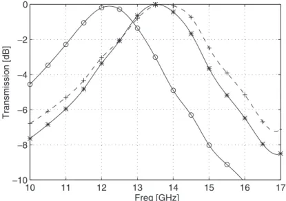
3.6 Predicted transmission coefficient of an O-ring FSS with one side perspex only. . . 39

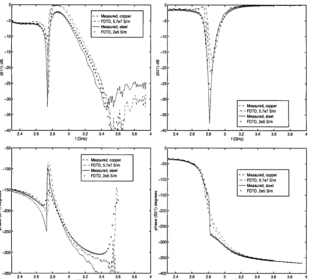
3.7 Measured and predicted scattering parameters for copper and steel unit cells of cranks (chiral hooks) in polystyrene foam. . . 41

3.8 Prof Johannes Cloete and a group of the first doctoral graduates from the SU Electromagnetics group. . . 44

4.1 The right-angled parent triangle. . . 47

4.2 The three Whitney basis functions for triangles. . . 49

4.3 A doubly-coated graphite aerofoil. . . 51

4.4 The bistatic RCS of the coated aerofoil as a function of incidence angle. . . 52

4.5 A tetrahedral mesh with 1001 elements. . . 55

4.6 The capacitive iris. . . 56

4.7 Results for a capacitive iris as a function of mesh size. . . 56 x

(12)

4.8 Results for a capacitive iris, as a function of degrees of freedom . . 58

4.9 Results for the half-cylinder pin filter geometry problem. . . 59

4.10 Tetrahedral hybrid mesh of the half-cylinder pin filter geometry. . . 60

4.11 Dr Gronum Smith, Dr Frans Meyer and the author. . . 63

4.12 The EMSS group in April, 2014. . . 64

5.1 Run-times for LU decomposition, compared for systems capable of sustaining 1 MFLOP, 1 GFLOP, 1 TFLOP, and 1 PFLOP. . . 66

5.2 Speedup using GPU . . . 70

5.3 A comparison of the processing capability of various systems inves-tigated by Ilgner. . . 71

6.1 The SKA group at Stellenbosch in March 2014. . . 74

6.2 The LOFAR array at Onsala Space Observatory, Sweden and FEKO model . . . 78

6.3 The Dense Dipole Array on the Stellenbosch University spherical near-field range. . . 79

7.1 The anechoic chamber coordinate system. . . 84

7.2 The antenna range at SU follow the upgrade. . . 85

7.3 A diagram showing the layout of the SU anechoic chamber. . . 86

7.4 An example of a redundant near-field measurement. . . 87

7.5 Far field patterns corresponding to redundant near-field measure-ments. . . 89

7.6 RMS disparity between computed far-field patterns . . . 90

7.7 Far-field cut with RMS envelop. . . 90

7.8 Contemporary photo of the KAPB. . . 91

7.9 Attenuation map for dishes facing 1 (facing southwest), stowed, at 1 300 MHz. . . 92

7.10 Attenuation map for dishes facing 1 (facing southwest), stowed, at 3 050 MHz. . . 93

(13)

List of Tables

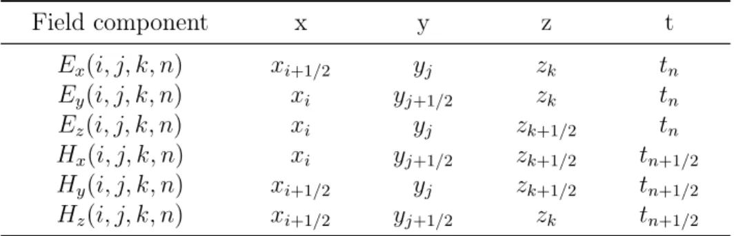
3.1 Spatial and temporal location of fields in 3D FDTD algorithm . . . 30 5.1 Computational throughput of the FDTD method on various HPC

platforms . . . 71

(14)

List of notation

Throughout this dissertation, the following notation is used. Spatial vectors are indicated asE(in this case, the electric field). Vectors in the linear algebra

sense are indicated as {x}, and matrices as [A]. The individual elements of a

vector or matrix are of course indicated as xi or Aij respectively. Otherwise, the notation is as generally encountered in engineering books on this topic. A summary is presented below.

The time convention used for phasor quantities isejωt_{, hence, an}_e−jkr _plane wave propagates in the direction of increasingr. (Note that physics texts often

adopt the e−iωt convention, in which case the sign also changes in the plane

wave exponential factor; engineering texts occasionally use e−jωt_{, which has} the same effect.)

∇× the curl operation

∇· the divergence operation

× the vector cross product of two vectors

E the (field) vector E

0 the permittivity of free space (≈8.854×10−12 F/m)

r relative permittivity of a dielectric material (dimensionless)

µ0 the permeability of free space (4π×10−7 H/m)

µr relative permeability of a magnetic material (dimensionless)

c the speed of light in free space (_≈2.9979_×108 _m/s)

λ wavelength (m/s)

λi simplex coordinate i

O(Mn₎ _{of the order of} _Mn_{, formally,}

N =_O(Mn₎_⇒ _lim

M→∞logN/logM =n

(15)

[A] the matrix A

aij the ijth element of matrix A

{x} the (algebraic) vector x

xi the ith element of vector {x}

||{x}|| the Euclidean norm of the vector {x} of length n,

||{x_{}|| ≡} pPn_i₌₁_|xi|2

≡ is defined as

∀ for all

|z_| absolute value of z

(16)

Chapter 1 Introduction

My research career started in 1983 as post-graduate student at the University of Pretoria, working on numerical methods for antenna analysis. The research that will be presented in this dissertation spans a career of more than thirty years to date in engineering electromagnetics, with a particular focus on com-putational electromagnetics through much of this period. As such, there is no more appropriate point to begin than with a brief discussion of Maxwell’s equa-tions, before moving on to preview the dissertation and provide some personal background in the rest of this introductory chapter.

1.1 Maxwell’s equations

Electromagnetics, the study of electrical and magnetic fields and their

interac-tion, has been one of the core technologies of the twentieth century, and shows every sign of continuing this into the twenty-first. Whilst there are many useful ways of subdividing the field, power frequency versus radio frequency, or alter-natively quasi-static versus full-wave, is one of the most insightful here. This dissertation focusses exclusively on radio-frequency, full-wave electromagnetic modelling, as typically encountered in communication systems, remote-sensing applications and radio astronomy telescopes.

The core of modern electromagnetic engineering is of course Maxwell’s equations. Written in modern form1, they are:

∇ ×E = ₋∂ ∂tB (1.1) ∇ ×H = J + ∂ ∂tD (1.2) ∇ ·D = ρ (1.3) ∇ ·B = 0 (1.4)

1_{Maxwell did not actually write his equations in this form; vector analysis was a late}

nineteenth-century development.

(17)

with the associated constitutive equations

B = µH (1.5)

D = εE (1.6)

Here, I follow the physics convention, regarding B as the primary magnetic

field; EandBare the relevant transform pair in the Lorentz transform

(Feyn-mannet al., 1963:Chapter 267, Volume II), and Bis the relativistic correction

of E, as Feynman very elegantly shows (Feynmann et al., 1963:Section 13.6, Volume II). The utility ofH in especially quasi-static engineering appliations,

such as the design of electrical machines, has led to its widespread usage in the electrical engineering literature as the primary magnetic field.

The actual solution of the Maxwell equations is complex, and for realistic problems, approximations are usually required. The numerical approximation of Maxwell’s equations, the subject of much of this dissertation, is known as

computational electromagnetics (CEM). During my career, CEM has emerged

from a few (largely US military) research laboratories into widespread deploy-ment in industry, and I have played a part in enabling this.

1.2 Contributions

The main body of work to be presented will be an overview of my own and my research group’s extensive publications on computational electromagnet-ics, which have advanced the field in a number of aspects. (They have also contributed materially to the success of the company Electromagnetic Soft-ware and Systems — now Altair.) Application of my research has shifted from primarily defence work (during the late 1980s, when I started my ca-reer) to my appointment to the Square Kilometre Array (SKA) South African Research Chair in Engineering Electromagnetics in 2011, in support of South Africa’s MeerKAT radio telescope and SKA program. The golden thread of my work has been modelling full-wave electromagnetic fields in increasingly complex environments. This has also now expanded to include work on ap-plying these methods to antenna design in the context of radio astronomy. My work also now addresses other topics in engineering electromagnetics, in-cluding calibration and imaging for radio astronomy (much of which leverages CEM simulations) and also antenna metrology and propagation modelling.

My core technical contribution to date has been the establishment of a coherent body of research, embedded in post-graduate training and publica-tion, addressing the theory and application of three main full-wave numerical methods used in RF and microwave engineering - the Method of Moments (MoM), Finite Difference Time Domain method (FDTD) and Finite Element Method (FEM), and significant industrial impact. At present, this includes over 60 peer-reviewed journal articles, over 150 conference presentations and

(18)

one text book in its 2nd edition. Over 50 graduate students and post-doctoral fellows have been supervised or co-supervised by me. A complete list of graduates to date may be found in Appendix A. Two of my doctoral grad-uates, Prof MM Botha and Prof RH Geschke, hold tenured positions at SU and UCT respectively, and other graduates were instrumental in the successful establishment and growth of Electromagnetic Software and Systems (of which the software business unit is now part of Altair). Details of research funding received may be found in Appendix B.

Particularly important advances and contributions, listed approximately chronologically2_{, include:}

• Pioneering work on parallel computing for the MoM using “commodity” processors — as opposed to very expensive vector supercomputers — including an efficient parallelized version of the then industry standard program NEC2 running on transputer arrays). Recently, this work has been revisited in the context of BlueGene supercomputers, GPGPUs and ARM processors on smartphones.

• Application of the FDTD to modelling optical devices and frequency selective surfaces.

• A long-running research program on the FEM with significant advances on the use of higher-order elements, error estimation, mesh termination (all of which have been successfully transferred to industry) and the first high-order hybrid explicit-implicit finite element time domain scheme. • My book on CEM, published by Cambridge University Press, now in its

2nd edition Davidson (2011).

• Work on new methods for the verification of CEM codes, using the method of manufactured solutions.

• Work on efficient CEM analysis methods for sparse arrays.

• Contributions to the SKA mid-frequency aperture array program, in particular via development of a new front-end prototype.

• Work on calibration and imaging, in particular including detailed an-tenna models into direction and baseline dependent interferometric imag-ing methods.

• The upgrading of SU’s antenna range with entirely new near-field capa-bilities, and a research program currently running on the evaluation of the chamber.

2_{There is inevitably overlap between substantial research efforts, and some ran in parallel}

(19)

These themes will be unpacked, with suitable references, in this disserta-tion.

1.3 Layout of the dissertation

This dissertation is presented in six main chapters. Chapters 2, 3 and 4 cover computational electromagnetics, addressing the MoM, FDTD and FEM re-spectively. As noted above, this development is approximately chronological, but my work on the MoM has spanned most of my career. Chapter 5 ad-dresses high-performance computing for CEM, and this work has been woven throughout much of my career. Chapter 6 and 7 present recent work, on radio astronomy and antenna metrology and electromagnetic propagation respec-tively.

1.4 My education, background and work

history

As this dissertation spans my entire career, some brief notes on my these topics appears appropriate. I was born in London, England in 1961 of a South African father and English mother. In 1968, my family moved to South Africa, where I was raised and educated, attending Pretoria Boys’ High School. My BEng, BEng (Hons) and MEng degrees were obtained at the University of Pretoria in 1982, 1983 and 1986 respectively. My PhD was obtained at Stellenbosch University in 1991.

My very first publications resulted from work I did with Jan Malherbe in 1983 (as an Honours student at the University of Pretoria) on the numerical integration of a mutual impedance integral and subsequent use in the design of a slot array (Malherbe & Davidson, 1984; Malherbe, Cloete, Losch, Robson

& Davidson, 1984); these are noted here, as they do not fit very readily into

subsequent chapters.

My compulsory national service was spent in the South African Army sig-nals corps (1984-85); following this, I worked at the Council for Scientific and Industrial Research in Pretoria as a research engineer, before being appointed in 1988 at the Dept of Electrical and Electronic Engineering at Stellenbosch University. I subsequently held the posts of Associate Professor (1992–5) and Professor (1996–2014) as Stellenbosch, as well as several temporary academic positions during sabbatical visits. As of January 2011, I have held the Square Kilometre Array Research Chair at Stellenbosch; this is part of the South African Research Chair Initiative (SARCHI) of the Department of Science and Technology (DST) and the NRF. As of July 2014, I also hold the position of Distinguished Professor at Stellenbosch University.

(20)

Figure 1.1: The title page of a paper by my father and my uncle from the

Trans-actions of the SAIEE, March 1957.

On a historical note, my father was also an electronic engineer, and worked in the telecommunications sector in the UK and South Africa for most of his professional life, after serving in the then Union Defence Force from 1942-1946 in the Special Signals Service (who were tasked with operating radars during WWII). I recently came across a paper from 1957 describing work he published

with a colleague3 _{from the UK on the microwave link from Johannesburg to}

Pretoria and reproduce the title page as Fig. 1.1.

3_{The second author (Bruce P Mackenzie) would subsequently become my uncle when}

his sister, Marguerite, married my father in 1959 in London. I take my second name from my uncle, so reproducing their paper here feels appropriate.

(21)

1.5 Closing comments

In closing this introductory chapter, the contributions which I will discuss in this dissertation have brought some recognition which I regard as significant. In 1996, I received the President’s Award from the NRF as a young researcher; I presently have a B1 rating. In 2012, I was honoured by the IEEE as a Fellow of the institute, with the citation For contributions to computational

electromagnetics. A more complete list may be found in Appendix C. As of

the time of writing, I have approximately 730 citations on Scopus, and 1 340 on Google Scholar4_{. The associated h-indices are 13 and 16 respectively.}

This would also be an appropriate point to mention my involvement in the profession. I have been involved in a number of professional activities, in particular via the IEEE, during my career. I chaired the South African IEEE AP/MTT Chapter from 1996–98. I served on the IEEE Antennas and Propa-gation AdCom (2011-’13), the IEEE APS Awards Committee (2009–2013) and the IEEE APS Fellows Committee (2014–16). I was General Chair of the 8th Finite Elements for Microwave Engineering Workshop, Stellenbosch, 2006 and Chair of the local organizing committee of ICEAA’12-IEEE APWC-EEIS’12, held in Cape Town in September 2012. (Since that 2012 conference, I serve on the steering committee of the ICEAA/IEEE APWC conference series). I am presently an associate editor of both the IEEE Antennas and Propagation Magazine and the IEEE Transactions on Antennas and Propagation. Addi-tionally, I have served on national committees in South Africa, including the NRF’s Engineering Assessment Committee in 2001–2002 (in the 2nd year as convenor), and again in 2006. My three-year term on the South African As-tronomy Advisory Council, a national body established by the NRF, has just ended.

4_{My long-standing role as Associate Editor of the IEEE AP Magazine results in a number}

of papers in the column I edit being incorrectly attributed to me on some databases; these have obviously been excluded from these figures as far as possible.

(22)

Chapter 2 Contributions to the MoM

2.1 Introduction

The Method of Moments (MoM) was historically the first numerical method widely adopted by antenna engineers. With the first papers appearing in the 1960s1, the method was ideal for application to highly conducting metallic

structures of resonant size. Early applications rigorously solved for the cur-rent distribution on a number of canonical antennas, such as log-periodic and Yagi-Uda antennas, widely used in telecommunications and for analogue TV reception (and indeed still in use today). The method was well suited to the limited computational capabilities of that decade. The MoM remains one of the most important numerical methods for antenna engineers to this day.

My work with the MoM, which I will outline in this chapter, has spanned much of my career, from my first graduate work right up to current applications in code testing and radio astronomy antennas. It is most easily presented in two main periods, the 1980s and 1990s, and more recent work (from the late 2000s onwards); during the 2000s, I focussed most of my research on the FEM, which is the topic of Chapter 4. To provide some background, the MoM is briefly reviewed in the following section, drawing on material from (Davidson, 2011:Chapter 4).

2.2 A very brief recap of the MoM

Starting from the decomposition of a time-harmonic electromagnetic field into incident and scattered fields, as

Etot =Einc+Escat (2.1)

1_{One widely used formulation, due to Pocklington, dates back to 1897, although his}

paper did not use a numerical method due to the obvious lack of automatic computers.

(23)

and using the representation of the electric field in terms of the magnetic vector potential A and electric scalar potentialΦ as

E=₋jωA_{− ∇}Φ (2.2)

it can be shown (see, for example, (Davidson, 2011:Chapter 4)) that for suf-ficiently thin wires, this can be reduced to the Pocklington equation, first introduced in 1897: Escat z (r) = 1 jω0 Z l/2 −l/2 ∂2_{ψ(z, z}0₎ ∂z2 +k 2_{ψ(z, z}0 ) Iz(z0)dz0 = −E_zi(r) (2.3)

This equation is obtained by assuming that we locate the filament on the axis and enforce the boundary condition on the surface (the reciprocal case is sometimes more convenient in deriving this). Although it looks fairly straight-forward, the presence of the second derivative of z inside the integral kernel,

acting on the Green function, makes this non-trivial to implement. A useful further simplification can be made if the wire is assumed very thin (aλ):

Z l/2 −l/2 Iz(z0) e−jkR 4πR5 (1 +jkR)(2R2₋3a2) + (kaR)2 dz0 =₋jω0Ezi(ρ=a) (2.4) withathe wire radius andR =pa2_{+ (z}₋_z0₎2. This is now a convenient form

to program. It appears in numerous texts — see, for example, (Balanis, 1989:p. 720) — and appears to have been first introduced by Richmond (Richmond, 1966), reprinted in (Miller et al., 1992).

The MoM proceeds by approximating the unknown (the axially-directed current Iz(z0) in this case) by a finite series approximation

I(z0)_≈

N X

n=1

anhn(z0) (2.5)

Here,anare unknown (but constant) coefficients, andhn(z0)arebasis functions – also often known as expansion functions.

At this stage, linear operator theory provides a convenient framework for developing the formulation (again, see for example, (Davidson, 2011:Section 4.5), from which this material is extracted). We introduce the equation

Lf =g (2.6)

where L is the operator which maps function f to function g. In the case of

Eq. (2.4), for instance, the function f is the axial current I; the function g is

(24)

Z l/2 −l/2 e−jkR 4πR5 (1 +jkR)(2R2−3a2) + (kaR)2 (·)dz0 (2.7)

The bracketed dot is used as a place-holder for the function on which this operator acts. Using this notation, the previous development then produces

L N X

n=1

anhn =g (2.8)

where, as before, f has been approximated using the basis functions, viz. f _≈

N X

n=1 anhn

Using point-matching, the N×N linear system can be obtained by testing the

above at N test points. But now, instead of doing this, we form the residual as: R=L N X n=1 anhn−g (2.9)

This residual is the difference between the approximate solution and the ac-tual solution. The point-matching procedure forces this residual to zero at N

discrete points. A better approach would be to try to obtain some type of average value of the residual over the domain of the problem (the length of the wire in this case), and set this to zero. One can do this in a quite general fashion by introducing the idea of a weighting function, which is multiplied by the residual (and hence the name, method of weighted residuals) and inte-grated over the domain. The weighting function (also often known as a testing function) is also usually expressed as some type of finite series:

w=

M X

m=1

wm (2.10)

In this case, the equality is appropriate, since we are not approximating this function. Note also that there are no unknown coefficients. Symbolically, the weighted residual method becomes

Z LR M X m=1 wmdz = Z L M X m=1 wmL N X m=1 anhn− Z L M X n=1 wng = 0 (2.11)

Usually, the number of basis functions (N) and the number of weighting

func-tions (M) are equal. Because this integration process frequently defines an

inner product, an equivalent notation frequently encountered is

(25)

This is of course the bracket notation widely used in quantum mechanics, for the matrix algebra formulation of Heisenberg. We will not pursue this further, other than to note that the reason for this analogy is that both classical electromagnetics and quantum mechanics are at heart field theories.

It is easy to show that the method of weighted residuals produces a matrix equation:

{V}= [Z]{I} (2.13)

with matrix entries

Zmn = hwm,Lhni

Vm = hwm, gi

In = an (2.14)

In addition to the question of which type of basis functions to adopt, one now can also choose a variety of weighting functions. This matter has been quite extensively researched. In practice, however, there are two very popular choices. The Galerkinprocedure uses the same basis and weighting functions. The collocation method, uses Dirac delta functions, which of course reduce to just testing the operator at the sample points.

The computational cost of filling the matrix (i.e. computing the entries of

Zmn) isO(N2); the cost of factoring the matrix isO(N3). The constants in the former can be quite large, depending on the accuracy of numerical integration (quadrature) required. The factorisation operation has constants of the order of unity.

For surfaces, the classic paper (Rao, Wilton & Glisson, 1982) introduced the use of vector-based triangular basis functions to solve the Electric Field Integral Equation. These basis functions are widely known in the CEM com-munity as the RWG element (after the authors, Rao, Wilton and Glisson). Following the same lines as the Pocklington equation, integral equations in either the magnetic or electric fields can be derived for problems with currents flowing on surfaces. One integral equation couples the incident electric field to the induced surface current, and is known as the electric field integral equation (EFIE): ˆ n_×Einc(r) = ˆn_× Z S [jkηJS(r0)G(r,r0) + η jk{∇ 0 s·JS(r0)}∇0G(r,r0) dS0, _∀r,r0 _∈S(2.15)

The ∇0 _{operator implies differentiation in the}_source_coordinates. _n_ˆ _{is the unit}

(26)

by

G(r,r0) = e

−jkR

4πR (2.16)

R = _|r₋r0_| (2.17)

Equation (2.15) is valid for both closed and open surfaces. In the latter case,

JS is the sum of surface currents on both sides of the sheet. A very widely-used form of the EFIE is the mixed potential integral equation (MPIE), which explicitly retains charge as an unknown. From the continuity equation — the time rate of change of charge is the negative of the divergence of the current — charge is of course connected to current, and this is exploited in the MPIE formulation.

A detailed development of an MoM solution using the RWG triangular basis functions may be found in the original paper (Rao, Wilton & Glisson, 1982), and this is reprised with some contemporary insights in (Davidson, 2011:Chapter 6).

2.3 Contributions during the 1980s and 1990s

2.3.1 M.Eng research: 1996

My initial research work in this field, undertaken at Master’s level was on radiation from aperture antennas mounted on conducting bodies of revolution (Davidson, 1986). The work was performed at the then National Institute for Aeronautics and Systems Technology (NIAST) of the Council for Scientific Research(CSIR) in Pretoria, South Africa. At that time, NIAST was the leading South African research centre for airborne defence technologies, and there was major interest in accurate modelling of aircraft and missiles, both for antenna positioning and radar cross section prediction, and bodies of revolution have obvious application here.

The BOR formulation is computationally very attractive, as it uses entire-domain Fourier modes to expand the circumferential variation of current, and only the generatrix needs be discretized. For rotationally symmetric excitation, only one Fourier mode is required. For other excitations, a relatively small number generally suffice (details are in the literature and my thesis).

The work was based on existing theoretical formulations using the method of moments (Mautz & Harrington, 1969), but the extension of the method to asymmetrical apertures was rather more complete than other published work; the theoretical work was also carefully supported using both measured results and results computed using the UTD. Additionally, theoretical methods for handling attached wires were considered in detail, as well as original theoretical work on near-field computation of the fields and the computation of coupling between antennas mounted on bodies of revolution. The work led to national

(27)

and international conference publications, and parts of the work was published nationally as (Davidson& McNamara, 1987) and internationally as (Davidson

& McNamara, 1988) and (Davidson & McNamara, 1989).

In terms of assessing this work, my Master’s research served as an excellent basis for subsequent research. The work was very well received for a Master’s thesis, as evidenced by the mark awarded, and perhaps more significantly from a research viewpoint, in the publications resulting from it.

2.3.2 Doctoral research: 1988–91

The original impetus for this work grew out of the experience obtained with the method of moments during the research for my Master’s degree, where problems where encountered with the limited electromagnetic size that was computationally tractable. As noted above, the computational cost is domi-nated by two terms, the matrix fill —O(N2₎_{— and the matrix solve —}_O(N3₎

using LU-type solvers. For iterative solvers, the cost isniterO(N2)for iterative solvers. (Here, N is the number of degrees of freedom in the simulation and,

where relevant, niter is the number of steps required for the iterative solver to converge adequately2_.)

N is frequency dependent: typically; at least 8–10 unknowns are required

per wavelength for wire problems (or this number squared per λ2 _{for surface}

problems). This places limits on the applicability of the method of moments, and for the computers typically available in late 1980s, these limits typically occurred some way before the structure was electromagnetically sufficiently large to use ray-based asymptotic formulations such as the UTD. This prob-lem had practical significance at the time since this “gap” in the coverage of techniques for typical aircraft and ground vehicles fell in the VHF commu-nication band — a most inconvenient place to be unable to predict antenna performance. (As subsequently become evident with later work on hybrid methods, the asymptotic techniques can be problematic to apply even when apparently appropriate, due to the nature of the approximate formulations, which is a further motivation for extending the MoM).

The research approach followed was firstly, to investigate the application of parallel computing to the problem of the matrix fill and matrix solve. The con-tributions here were efficient parallel conjugate gradient and LU decomposition algorithms. Then major parts of NEC2 were recoded in Occam 2, the “native” language of the T800 transputer (the technology available at the time). The matrix fill was parallelized, used the parallel CG and LU algorithms mentioned above. The culmination of my doctoral research was to demonstrate a version of NEC2 (called PARNEC) that could handle at least double the maximum number of degrees of freedom (segments in NEC2) when compared to that which could previously be handled using the most powerful serial processors

(28)

at the University3_{. Smaller problems that had previously required overnight}

runs could be solved in an hour or two following the doctoral work. This work was presented at five international and three national symposia and was published internationally as (Davidson, 1990, 1992, 1993).

In terms of assessing this contribution, this doctoral work (Davidson, 1991) remains some of the most significant, original research that I have been under-taken personally. Subsequent work (with the exception of much of my book, discussed in Section 4.5) has inevitably been undertaken either in a supervi-sory capacity or collaboratively. With hindsight, the research appears obvious, which can be taken as a measure of the success of the work. When the research was initiated in late 1988, very little had been published on suitable parallel algorithms — indeed, parallel versions of some of the algorithms did not even exist. This research was multi-disciplinary, since it involved electromagnet-ics, applied mathematics and computer science, and this fact attracted most favourable comment from the examiners. Another important aspect was the careful separation of the underlying principles of the algorithms from the com-puter technology used to implement the algorithms. Hence the analysis was suitable for the general class of local memory MIMD computers. The demon-strated scaling properties of the algorithms were also significant. Again, this was very favourably received by the examiners. Two invited published tutori-als on parallel processing for computational electromagnetics (Davidson, 1990) and (Davidson, 1992), and a journal paper (Davidson, 1993) resulted from this work; the first has been quite widely cited in the CEM literature.

One of the results of the PhD was that the speed-up and efficiency of a par-allelized MoM implementation depended fundamentally on the “grain” of the problem, where grain is a measure of the number of unknowns per processor. In most problems of interest, there are far more degrees of freedom that there are processors, so some decomposition (mapping) of the problem is required. For an iterative algorithm, a simple row-block or column-block decomposition is sufficient, but for an LU algorithm, an interleaved decomposition achieves better load balancing (at least in the absence of extensive pivoting).

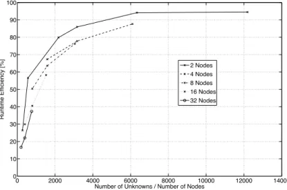
Examples of measured efficiencies on a transputer array are shown in Fig. 2.1. (The results are shown for slightly different numbers of processors; this was due to different interconnection topologies used for the algorithms.) These data were measured in the early 1990s on a transputer array, hence the problem sizes are small by contemporary standards, but nonetheless, es-tablish the principle. More contemporary results are shown in Fig. 2.2; these results were measured in 2009 using a parallel version of FEKO 5.3, run-ning on the IBM e1350 cluster installed at the Centre for High Performance Computing (CHPC), Cape Town, South Africa. This cluster had 160 nodes, each with two dual-core AMD Opteron 2.6GHz processors, and 16GByte of

3_The _O₍_N3₎ _{computational dependence should be borne in mind — a problem with}

(29)

0 50 100 150 200 250 0 10 20 30 40 50 60 70 80 90 100 N/P E ffi ci en cy ( % ) P=2 P=6 P=14 P=30

Figure 2.1: Measured efficiency of a parallel CG algorithm on a transputer array,

for an MoM problem with a total of N unknowns running on P processors. (After

(Davidson, 1993:Fig. 7).)

RAM, giving a total of 640 processors with a peak processing power of around 2.5 TFLOP and 2.56 TBytes of RAM. The system had both 1GBit/s Ethernet and 10GBit/s Infiniband interconnects. (Although faster, the latter was not as widely supported in application programs). The massive increase in unknowns is immediately apparent, driven by two decades of Moore’s Law.

(30)

0 2000 4000 6000 8000 10000 12000 14000 0 10 20 30 40 50 60 70 80 90 100 Runtime Efficiency [%]

Number of Unknowns / Number of Nodes 2 Nodes 4 Nodes 8 Nodes 16 Nodes 32 Nodes

Figure 2.2: Efficiency vs. grain size on on an IBM e1350 cluster, using the

(31)

2.3.3 Penetrable BOR modelling: 1990–4

My M.Eng work on the BOR was extended by my doctoral student Pierre Steyn during the period 1990-4. He extended this to include electromagnet-ically penetrable bodies in his doctoral dissertation (Steyn, 1994). This had important industrial applications for a number of antenna structures such as coated or radome-covered monopoles, for which no analytical or efficient nu-merical approach previously existed. In assessing this contribution, Dr Steyn did a meticulous piece of work on a difficult problem, and a paper on an aspect of the work won a prize at the local SUPEES ’93 symposium. We published the core results of his thesis as (Steyn & Davidson, 1995).

2.3.4 MoM simulation work for industry 1990–1998

During and following the doctoral work, a substantial amount of contract-oriented industrial simulation work was undertaken. This used the MoM tools which had been developed with colleagues and students. A project on using NEC2 and PARNEC for modelling vehicle mounted antennas ran from 1990 to the 1994. This work was primarily for the military, concentrating on ground vehicles and ships; a close relationship was developed with the SA Navy at Simonstown and Silvermine during this period. Much of this work was clas-sified to some or other extent; some unclasclas-sified and representative work was reported in (Davidson & du Toit, 1991).

In 1996 this was followed by my successful request via the US DoD for NEC4, which at the time of writing (over 20 years later) is still restricted US military technology. With final-year project student Toit Mouton4_{, the use of}

NEC4 for communication with submerged objects was investigated; a variety of problems were found, the solutions of which led via the complexities of Sommerfeld integrals to a paper on the topic (Davidson & Mouton, 1998).

In assessing this work, it led to a variety of technological innovations, the most significant being the successful NEC pre-processor WIREGRID, origi-nally developed for this research. It was published as (du Toit & Davidson, 1995). WIREGRID went through several subsequent re-writes, and became the first product of start-up company Electromagnetic Software and Systems, EMSS (who eventually discontinued the product, as their focus on FEKO deepened). Over the next twenty years, EMSS would grow to become a very substantial company; my interaction with EMSS will be described in detail at the end of Chapter 4.

2.3.5 Hybrid MoM/UTD work: 1997–1999

During the eighteen month period October 1997 – March 1999, Dr Isak Theron was a post-doctoral associate at the University. He worked with me on

(32)

brid UTD/MoM formulations — work that also flows from the same type of problems that were addressed in the author’s own PhD. This work was done specifically with Dr Ulrich Jakobus, then of the Univ. of Stuttgart, in ex-tending the FEKO MoM simulation program which he originally wrote for his PhD. (This work was also partially sponsored by EMSS.) In (Theron et al., 2000), we presented an extension to the uniform geometrical theory of diffrac-tion (GTD) for reflecdiffrac-tion from smooth curved surfaces. This approach allowed the source to be much closer to the reflecting surface than the conventional uniform GTD formulation and did not require a Hertzian dipole source. In essence, the field point was mirrored in the plane tangential to the specular (reflection) point; the incident field was then calculated at the mirror point and the uniform GTD reflection coefficients were used to mirror this field to the original field point. This formulation reduced exactly to the conventional uniform GTD if the incident field was ray optical. The application to a hybrid method of moments (MoM)/GTD code was outlined and results computed were presented for a dipole radiating in the vicinity of a cylinder.

This collaboration with Dr Jakobus would subsequently expand into a very substantial research program.

During essentially the same period, an M.Eng student, Sven Keunecke, whose thesis topic was also in this general area, was also supervised by the author. A paper based on some examples from his M.Eng thesis was pub-lished as (Davidson & Keunecke, 1999) which was a useful tutorial summary of various various MoM/asymptotic hybrid techniques. Some of this work was revisited in (Davidson, 2011:Chapter 6). Quite recently, I revisited this topic with Siyanda Nazo, who Master’s thesis addressed hybrid formulations using large element physical optics (Nazo, 2012).

In assessing this work, Dr Theron and I eventually found the MoM/UTD hybridisation somewhat frustrating; the UTD is a powerful method for a suit-able, but very restricted, class of problems, but we found the meaningful ex-tension of it to the rather more arbitrary problems that one wants to address with a general purpose simulation code essentially intractable. Several con-ference publications resulted from this work; the most important result, for the special case of a dipole radiating near a cylinder, was published as noted above.

2.3.6 Other contributions - spectral domain MoM work,

1997–1999, Sommerfeld formulations, 2002–2003

Whilst my work in the 2000s turned very much to the Finite Element Method, I continued to do some work with the MoM; work on introducing the spectral domain MoM formulation was publshed in (Davidson & Aberle, 2004), sev-eral years after a collaboration with Prof Jim Aberle involving a short course initiated the work. More significantly, this led me to study the Sommerfeld

(33)

for-mulation in depth, and to present a guide to a single-layer implementation in my textbook. This represented a substantial educational contribution, which will now be briefly described.

Due to its perceived complexity, the topic of stratified media (and the re-sulting Sommerfeld potentials) is generally regarded as an advanced one, and the coverage tends to be highly theoretical, and frequently impenetrable with-out lengthy study. One reason for this is that historically, analysis focussed on the problem of a dipole above a dielectric half-space. There are a number of complex issues which this raises, requiring quite sophisticated analytical techniques to understand, in particular for the asymptotic cases where inter-esting radiation physics can be extracted. However, the analysis of a very important special case, namely the grounded single-layer microstrip line (or patch antenna), can be undertaken without undue complexity, at least for most practical cases where the substrate is relatively thin.

The chapter in my book (Davidson, 2011:Chapter 7) starts with a static analysis of a microstrip transmission line, to demonstrate the basic principles of the spectral domain and the derivation of the Green function. Following this, the electrodynamic analysis is introduced, and the Sommerfeld poten-tials are derived from first principles. An extensive discussion of the numerical evaluation of the Sommerfeld potentials is presented. This is then brought together in an MoM analysis of a printed dipole using entire domain basis functions; some results are shown in Fig. 2.3. (A number of approximations made in the implementation limit accuracy, and the interested reader is re-ferred to (Davidson, 2011:Fig. 7.13) for further discussion.) Although most the work in this chapter is not original, being based on a synthesis of the liter-ature — in particular (Mosig, 1989) — the presentation in the present format does not appear to have been thus undertaken in other works before mine. I have had good feedback from those dedicated enough to work through the details of the chapter!

(34)

7 7.5 8 8.5 9 9.5 10 10.5 11 −20 −18 −16 −14 −12 −10 −8 −6 −4 −2 0 Freq [GHz] | Γ | [dB]

This code (fine) This code (coarse) FEKO

Figure 2.3: Reflection coefficient of a thin printed dipole. After (Davidson,

(35)

2.4 Recent work on MoM — late 2000s

onwards

2.4.1 The Method of Manufactured Solutions

My recent focus on radio telescopes led to a renewed and strong interest in the MoM. Marchand’s PhD dissertation (2013) represented some very sophisti-cated work on verifying CEM codes using an approach not previously published in the CEM literature, called the Method of Manufactured Solutions (MMS). In essence, the idea is obvious — provide what is usually the unknown in the problem (eg. the surface current, for a typical MoM code) and then compute from that what would usually be the known driving function or boundary con-dition (the incident field, ditto). For example, in eq. (2.15), the surface current

JS(r0) is chosen, and from the EFIE, the tangential electric field nˆ×Einc(r) is computed. This field is then used to drive an MoM solution, from which

JS(r0) is computed. This solution can now be compared with the original manufactured solution. It should be noted that this manufactured solution and associated incident field do not need to represent a physically realizable current or field. However, the MS should be chosen appropriately, for instance normally directed current must go to zero at the edge of thin plates.

For the FEM, this turned out to not be too difficult. However, the MoM raised a veritable cornucopia of tough problems, ranging from needing highly accurate quadrature schemes to appropriate norms. (It transpires that when investigating the convergence of MoM solutions, the widely-usedL2norm is not

sufficiently rigorous. One needs to use results from negative fractional Sobolev spaces to better evaluate the norm.) Rates of convergence are also crucial for verifying codes — subtle errors are often only revealed by a careful convergence study — and for the MoM, this is a complex issue. Work over the last two decades in the applied mathematics community has provided results for specific classes of geometry — (Buffa & Christiansen, 2003) and (Christiansen, 2004) are important contributions in this regard — and we used some of these. The core results were published in a special section on Validation of Computational Electromagnetics in the IEEE Trans on EMC (Marchand & Davidson, 2014); in my recent NRF rating application, I rated this as one of my my five best research outputs in that period, and I rate it as one of my career best. I also contributed quite extensively to the actual writing of the paper.

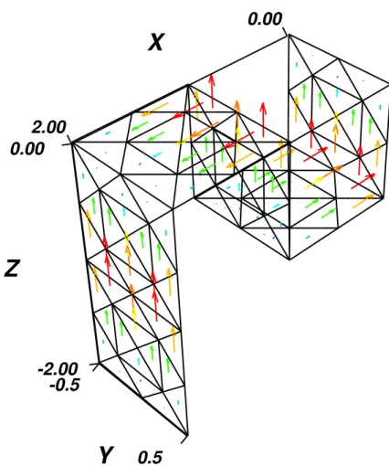
The key advantage of the MMS over canonical solutions is that a much wider range of geometries can be addressed, and hence more code capabilities are exercised than is the case with the classical approach of canonical solutions (which are extremely limited in number). For the types of accuracy required, measured solutions are also often inadequate. An example of the application of this method is the ribbon-line geometry show in Fig. 2.4. The MS is chosen as

(36)

-0.5

-2.00

Y

0.5 Z

0.00

2.00 X

0.00

Figure 2.4: Ribbon-like geometry and visual plot of an appropriate manufactured

solution (as in the text), after (Marchand & Davidson, 2014:Fig.5).

J =nˆ_×fh, (2.18)

with

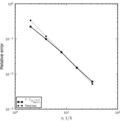
fh = (cos(xπ) + cos((z+ 1)π))ˆy (2.19) A comparison of the expected rate of convergence with that actually computed is shown in Fig. 2.5. It should be emphasized that this MS is not a physical solution of the Maxwell equations subject to the boundary conditions on the ribbon, but a solution chosen to exercise the code. (In this case, some defi-ciencies in the MoM implementation were revealed by the process, showcasing the utility of the method. Our application of the MMS also revealed a subtle error in a publicly available FEM package.)

2.4.2 GPU acceleration of the MoM

High-performance computing for CEM (the topic of my own 1991 PhD) was epitomised by the PhD dissertations of (Lezar, 2011) and (Ilgner, 2013), and

(37)

100 ₁₀1 ₁₀2 ∝1/h 10−3 10−2 10−1 100 Relativ e error k · k_H−0.5 div(Γ) Trend line

Figure 2.5: Computed convergence rate for the manufactured solution above,

com-pared the expected trend line with slope 3/2. In this figure, the wavenumber multi-plied by the maximum mesh element size (k0 h) ranges from 0.16 to 0.01. The upper curve is computed with the correct negative fractional Sobolev norm alluded to in the text. After (Marchand & Davidson, 2014:Fig.6).

this will be revisited in more detail in Chapter 5. Lezar worked on GPU implementations of both MoM and FEM codes; the key results are presented in (Lezar & Davidson, 2010b,a). At the time of writing, the latter paper is my fifth most highly cited paper, and taken together, these two papers have almost 100 citations on Google Scholar; an excellent example of how early publications on a “hot” topic can generate a large number of citations in short order.

(38)

2.4.3 Efficient analysis of large finite arrays - the

Domain Green’s Function Method

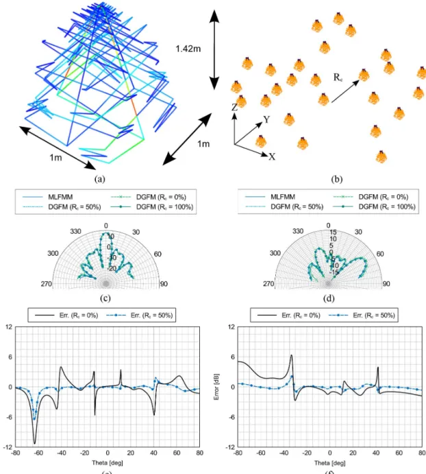
Ludick’s PhD dissertation (Ludick, 2014) continued work he originally ad-dressed in his MSc thesis (Ludick, 2010). This work, the first here which specifically focusses on the application of CEM to problems in radio astronomy, addressed the issue of large, but finite unconnected arrays (examples include the MWA, LOFAR and SKA-low). Using a novel method called the Domain Green’s Function Method (DGFM) approach, it proved possible to obtain both accurate and computationally cheap solutions for appropriate problems. In its basic form, the DGFM assumes initially that the current on each array ele-ment has the same relative spatial distribution, but with potentially different amplitude and phase, as per the feed weighting. Using a block decomposition of the overall MoM matrix, the currents on each array element can then be computed using the “active impedance matrix”, which takes both self-coupling and mutual coupling into account, the latter albeit approximately. The solu-tion thus obtained permits the computed currents to depart from the initial assumption of idential spatial distribution. An improved method was also im-plemented, which relaxed the assumption of identical current shape, and a further iterative extension was proposed in (Ludick et al., 2016). Some of this work was done in collaboration with Chalmers Univ of Technology, and resul-tant publications have elucidated the connection with the Characteristic Basis Function method. This work has already been incorporated into commercial simulators, and (Ludick et al., 2014) serves as a good reference for the most important results. Fig 2.6 from that paper shows results examining the effect of the “radius of convergence”, introduced by Ludick to limit mutual coupling

computation (and hence accelerate the method). Rc = 0% implies no mutual

coupling between array elements is taken into account, Rc = 100% that all mutual coupling terms are (albeit approximately, subject to the DGFM as-sumptions). The results are computed for a “zig-zag” element, which is has similarities with the current SKA-Low antenna prototype. Fig 2.7 applies the method to a much larger array, more typical of likely station sizes for SKA-Low.

It also showcased increasing international collaboration, including the leg-endary Prof Raj Mittra, who had been impressed by a presentation by Ludick on his Master’s work, and Dr Rob Maaskant, then rapidly establishing a rep-utation for his work on the CBFM method. Ludick is now continuing further work on this and other antenna-related topics in his post-doc.

(39)

Figure 2.6: Application of the DGFM to a Zig-Zag antenna displayed in (a), in

an array configuration displayed in (b). The directivity patterns for scan-angles of

(θ = 0◦, φ = 0◦) and (θ = 60◦, φ = 0◦) are presented in (c) and (d), respectively.

The errors in the directivity for different Rc values are presented in (e) and (f),

where Rc= 100% is used as reference. All results are obtained for the active array

environment where all the elements are excited equally and simultaneously. (a) Dual-polarized Zig-Zag element geometry. (b) Array configuration containing 26 irregularly spaced Zig-Zag elements. The element spacings ranges from λ/2 to 3λ,

at an operating frequency of 70 MHz. (c) Total directivity pattern (dBi) for a scan-angle of (θ = 0◦_{, φ} _{= 0}◦₎_{. (d) Total directivity pattern (dBi) for a scan-angle of}

(θ = 60◦, φ = 0◦). (e) Error (dB) in the calculated directivity for Rc = 0% and

Rc = 50% compared to Rc = 100%. Considered scan angle: (θ = 0◦, φ = 0◦).

(f) Error (dB) in the calculated directivity for Rc = 0% and Rc = 50% compared

to Rc = 100%. Considered scan angle: (θ = 60◦, φ = 0◦). After (Ludick et al.,

(40)

Figure 2.7: Applying the DGFM to a Zig-Zag antenna shown in Fig 2.6a, in a

529-element array configuration. The gain patterns for scan-angles of (θ = 0◦, φ = 0◦)

and (θ = 60◦, φ = 0◦) are presented in (b) and (c), respectively. (a) Array

config-uration containing 529 irregularly spaced Zig-Zag elements. The element spacings ranges from λ/2to 3λ, at an operating frequency of 70 MHz. (b) Total gain pattern

(dB) for a scan-angle of(θ= 0◦, φ= 0◦). (c) Total gain pattern (dB) for a scan-angle

(41)

2.5 Conclusions

Looking back, my very first encounter with the computational electromagnetics was an introduction to the MoM in 1983, during a post-graduate course taught by Prof Jan Malherbe at the University of Pretoria. Factoring a three-by-three complex matrix on a programmable HP pocket calculator (an HP-41CV) led me to a very early appreciation of computational cost5_{, a factor which}

has driven much of my work in especially the MoM throughout my career to date, with the use of high-performance computing platforms a recurring theme. Related to that is the requirement to improve modeling fidelity, which has been another significant driver — most recently epitomised by the work on the method of manufactured solutions.

In assessing my contributions to the MoM, citations can be useful, and the work Lezar and I published on GPU-acceleration of MoM codes is amongst my most-cited work, but some other very fine work, such as the MMS papers, has only very recently come to the attention of the community. Another significant factor, which citations do not gauge, has been a very close relationship with industry, in particular EMSS-SA. A number of topics originally undertaken as research have been successully commercialised, in particular in the FEKO simulation package. My first boss, Dr Dirk Baker, used to comment that “the best way to transfer technology is on two legs”, and a very large number of my former students at EMSS and Altair attest to this.

As one’s career progresses, it is most gratifying to see former student be-come leading researchers in their own right. In the context of the MoM, it is appropriate to mention the career of Dr Matthys Botha6_{. His doctoral work}

will be described later in this document as it was largely on the FEM, but his later postdoctoral work, and his subsequent work as an independent researcher, increasingly focussed on the MoM, so it is appropriate to note it here. During his post-doc with me in 2004–2005, he initiated work on both volume integral equations and higher-order divergence conforming elements (generalisations of the RWG element discussed earlier in this chapter) and published two excel-lent papers on these (Botha, 2006, 2007). Dealing with higher-order elements immediately focusses one’s attention on the problem of integrating both the singular and near-singular kernels which occur in the MoM formulation — ironically, the latter is often more challenging — and Botha’s formidable abil-ity was drawn inexorably to this problem, finally publishing another excellent paper on this topic which synthesised several years’ work (Botha, 2013). Cur-rently, he is working on improved Physical Optics formulations, with very promising results.

Whilst the MoM is an extremely powerful method, it is at its best dealing with highly conducting surfaces (or homogenous material structures).

Inhomo-5_{This process took several minutes!}

(42)

geneous material structures are often better addressed with differential-based methods, in particular the FDTD and the FEM. After completing my PhD, my own attention was drawn to these methods, as new challenges in dealing with complex material structures arose. I would work on these myself, and also supervise numerous students, more or less up to the present. In the next chapter, I discuss my work on, and contributions to, the FDTD.

(43)

Chapter 3 Contributions to the FDTD

3.1 Introduction

During the late 1980s and early 1990s, the Finite Difference Time Domain (FDTD) method became an extremely popular method. This was due to several factors. On the one hand, there were technology pushes, such as al-gorithmic advances, and the dramatic increases in computational power and RAM available on personal computers (and also workstations); on the other hand, there were application pulls, in particular the widespread deployment of low observable (“stealth”) technology in the military, and public concerns about exposure to non-ionizing electromagnetic radiation from cell-phones, the use of which was growing dramatically at that time. Both of these applica-tions involve highly inhomogeneous, electromagnetically penetrable materials, for which the MoM was far from ideally suited. Diffferential-based methods, in particular the FDTD, proved very suitable for this type of problem.

3.2 A brief overview of the FDTD method

As with the preceding chapter, this chapter starts with a brief overview of the method under discussion, which in this case is the FDTD. The following is excerpted from (Davidson, 2011:Chapters 2 & 3).

The finite difference time domain method, usually referred to as the FDTD, is a particular implementation of a general class of methods known as finite dif-ference techniques. The FDTD is so widely used in the CEM community that although finite difference methods cover a wide spectrum of complexity and accuracy, it is the FDTD which is almost always implied in CEM when finite differences are mentioned. Finite difference methods are numerical methods in which derivatives are directly approximated by finite difference quotients. The general class of such methods is the most intuitive numerical approach, and was the first to be extensively developed by the scientific computing community.

(44)

To this day, it probably remains the most universally applicable numerical technique and the one most widely used for scientific computation.

The FDTD method was introduced by (Yee, 1966) at much the same time as the original papers on the MoM appeared. However, the computational requirements of the full 3D algorithm were extremely high for 1960s-era com-puters, due to the requirement to fully discretize both the radiator/scatterer and a substantial volume of free space around it, and it was around a decade before Taflove was to develop the method further, also coining the term FDTD. (The original Yee paper does not use that name).

The FDTD is an initial value method, using a central difference approxima-tion for both the temporal and spatial derivatives. This provides second-order accuracy — but at the cost of two grids, offset in both time and space, which is a complication always to bear in mind with FDTD formulations. For the full three dimensional FDTD all six field components must be considered. The field components are located on the full Yee cell, described in the next section. The field components are offset in both space and time. Details are available in a number of texts; the most widely referenced and comprehensive text remains (Taflove & Hagness, 2005).

For a 3D FDTD code, memory is a serious issue; the storage requirements for the six field components (times two, for past and present) and the material arrays (in double precision) become 144Nx×Ny×Nz bytes. A computational volume with 100 cells on a side will require 144 MB. This will run easily on con-temporary personal computers (depending obviously on the amount of memory installed); doubling this to 200 cells in each direction increases the memory re-quirement to well over 1 Gbyte, still within the scope of most PCs at the time of writing; but doubling this again will most likely exceed available capacity. Double precision is unnecessary for many applications, and one can save stor-age by storing an integer index rather than the material arrays; similarly, in many applications, the fields can be overwritten immediately, approximately halving storage requirements; but even so, the storage requirement grows very rapidly.

The computational cost associated with fully discertising three dimensions should also be noted. The computational complexity of the algorithm is O(N)4_{, but in terms of electromagnetic size, it is} _O_(k

maxd)5–O(kmaxd)5.5, due to the necessity of controlling numerical dispersion. Halving the mesh size increases the run time by a factor of 16; doubling the frequency, by between 32 and 45 or so, when numerical dispersion is correctly controlled1_.

It is for these reasons that the development of efficient ABCs was so cru-cial as the enabling technology which permitted widespread adoption of the FDTD. Highly efficient ABCs permit one to place the scatterer very close

1_{See (Davidson, 2011:Section 1.4), for a discussion of dispersion in FDTD grids, and}

how controlling it as computational volumes grow in size requires increasing mesh density, as noted above.

Contributions to engineering electromagnetics

by

David Bruce Davidson

Dissertation presented for the degree of Doctor of

Engineering (Electrical and Electronic Engineering) in the

Faculty of Engineering at Stellenbosch University

Declaration

Abstract

Contributions to Engineering Electromagnetics

Uittreksel

Acknowledgements

Dedication

Contents

List of Figures

List of Tables

List of notation

Chapter 1

Introduction

1.1

Maxwell’s equations

1.2

Contributions

1.3

Layout of the dissertation

1.4

My education, background and work

history

1.5

Closing comments

Chapter 2

Contributions to the MoM

2.1

Introduction

2.2

A very brief recap of the MoM

2.3

Contributions during the 1980s and 1990s

2.3.1

M.Eng research: 1996

2.3.2

Doctoral research: 1988–91

2.3.3

Penetrable BOR modelling: 1990–4

2.3.4

MoM simulation work for industry 1990–1998

2.3.5

Hybrid MoM/UTD work: 1997–1999

2.3.6

Other contributions - spectral domain MoM work,

1997–1999, Sommerfeld formulations, 2002–2003

2.4

Recent work on MoM — late 2000s

onwards

2.4.1

The Method of Manufactured Solutions

-0.5

-2.00

Y

0.5

Z

0.00

2.00

X

0.00

2.4.2

GPU acceleration of the MoM

2.4.3

Efficient analysis of large finite arrays - the

Domain Green’s Function Method

2.5

Conclusions

Chapter 3

Contributions to the FDTD

3.1

Introduction

3.2

A brief overview of the FDTD method