Design and Testing of a Controller for Autonomous Vehicle Path Tracking Using GPS/INS Sensors

(1)

Design and Testing of a Controller for Autonomous Vehicle Path Tracking Using

GPS/INS Sensors

Juyong Kang*. Rami Y. Hindiyeh**

Seung-Wuk Moon***, J. Christian Gerdes****, Kyongsu Yi*****

*School of Mechanical and Aerospace Engineering, Seoul National University, Seoul, Korea

**Department of Mechanical Engineering, Stanford University, Stanford, CA94305 USA(e-mail: [email protected] )

***School of Mechanical and Aerospace Engineering, Seoul National University, Seoul, Korea ****Department of Mechanical Engineering, Stanford University, Stanford, CA94305 USA(e-mail: [email protected] )

*****School of Mechanical and Aerospace Engineering, Seoul National University, Seoul, Korea(e-mail: [email protected] )

Abstract: This paper describes a steering controller integrated with speed controller for autonomous path tracking using GPS and INS sensors. The steering controller for path tracking is developed based on the finite preview optimal control method. The steering control input is computed using the road information within preview distance. The speed controller determines the speed command necessary to maintain a lateral acceleration limit and improve vehicle safety. The vehicle model for simulation study is validated using vehicle test data. Finally, the controller is implemented on a by-wire vehicle, P1, to validate the performance of the steering controller integrated with speed controller.

1. INTRODUCTION

Intelligent Vehicle and Highway System (IVHS) technologies have attracted growing attention among researchers throughout the world in the past several years. Control algorithms for autonomous vehicles, including proper control of the steering input and speed commands for path-tracking and safe lateral vehicle behavior, are a critical component of IVHS (Peng, 1992, Hesss et. al. 1990).

In this paper, a steering controller for path-tracking and a speed controller for improving the safety of lateral vehicle behavior are investigated. The steering controller is developed based on the finite preview optimal control method. The steering input of the steering controller consists of a feedback control input using lateral position and yaw angle error as well as a feed-forward control input computed using the road information within the preview distance. The feed-forward preview control input can improve not only the tracking performance of the steering controller, but also the ride quality compared with the non-preview controller. (Kim

et. al., 2007)

The speed controller computes a speed command so that the lateral acceleration of the test vehicle does not exceed an arbitrary critical value in order to improve the safety of lateral vehicle behavior.

A vehicle simulation that includes lateral vehicle dynamics, longitudinal vehicle dynamics, and actuator dynamics is used to develop the controllers. The controllers developed are then implemented on a steer-by-wire test vehicle, P1, and validated experimentally.

2. TEST PLATFORM

The steering controller integrated with speed controller has been developed for P1, a student built by-wire platform

belonging to the Dynamic Design Lab at Stanford University, shown in Fig. 1.

Fig. 1. “P1” experimental by-wire vehicle

This vehicle features throttle by wire and independent left and right steer-by-wire at the front wheels. P1’s powerplant consists of two AC propulsion motors that provide independent left and right rear wheel drive as well as regenerative braking capability.

P1’s sensor suite includes a three antenna GPS system and standard automotive grade INS sensors. Real-time state estimation is accomplished through sensor fusion via extended Kalman filters for heading, velocity, and position

(Ryu et. al., 2004). A GPS base station has been used to

provide differential corrections for position measurements. 3. VEHICLE MODEL AND MODEL VALIDATION

3.1 Vehicle Model

The vehicle simulation was designed as an alternate mode for the SIMULINK software that normally runs in real-time on the test vehicle. It replaces hardware drivers with a vehicle model that creates “sensor” signals that are processed in the same manner as they would be in real time on the vehicle. This facilitated remote development of controller for the test platform by researchers at Seoul National University.

(2)

The simulation includes lateral, longitudinal, and steering actuator dynamics, as described below.

Lateral Dynamics:

P1’s lateral dynamics have been modelled using a four wheel planar model (Gadda et. al., 2007), as shown in Fig. 2 below:

yfl F Fyrl r l f l ε x v y v yfr F fl δ fr δ w t Fyrr

Fig. 2. Four wheel planar model

The equations for the lateral dynamics are given below,

(

)

(

)

y x yfl yfr yrl yrr

z f yfl yfr r yrl yrr

m v

F

I

l

F

l

F

ε

⋅ + ⋅ ⋅ =

+

⋅ = ⋅

+

− ⋅

+

(1)

where lf and lr are the distances of the front and rear axles from the CG, Iz is the moment of inertia, m is the vehicle mass, and Fyfl, Fyfr, Fyrl and Fyrr are the lateral tire forces at the front left, front right, rear right, and rear left tires, respectively. The lateral tire forces are linear functions of slip angles α_f and

α

_r and cornering stiffnesses C_f and C_r.

; , , ,

yi i i

F =C ⋅

α

i= fr fl rr rl (2) Using a small angle approximation, the tire slip angles are

as given in the expressions below, where

t

_w is the track

width of the vehicle. Vehicle parameters are given in Table.1.

, ; , / 2 / 2 y f y r fj fj rj x w x w v l v l j l r v t v t ε ε α δ α ε ε + ⋅ − ⋅ = − = − = ⋅ ⋅ ∓ ∓ Longitudinal Dynamics:

The model of longitudinal dynamics maps a voltage command to motor torques (

τ

_m) using simple models of P1’s traction battery pack, inverters, motors, and gearboxes. These motor torques serve as an input into a simulation of longitudinal dynamics that accounts for transmission inertia (J_trans), wheel inertia (J_wheel), rolling resistance, and the drag force (τ_air) acting on P1. This longitudinal model assumes zero wheel slip and no coupling with lateral dynamics; for the levels of lateral acceleration under consideration (<0.5g), these assumptions are reasonable. Equation (3) presents the equations for the model of P1’s longitudinal dynamics,

2 ( )

,

(4 2 ) /

t m air roll

x x x

wheel trans chassis

n a v a dt J J J r τ τ τ ⋅ ⋅ − − = = ⋅ + ⋅ +

∫

(3)

where,

r

denotes the tire rolling radius, n_t the drive ratio, chassis

J the chassis inertia and

a

_x the longitudinal acceleration. Steering System Dynamics:

A simple second order model is used to describe the output

shaft angle

θ

of P1’s left and right steering motor and

gearbox assemblies,

( / )Js η θ= −fssgn( )θ −bsθ+(1/ )(ns τaligning+τjacking)+k IM in (4)

where

J

_s is the effective inertia being acted upon by the

motor,

η

the motor efficiency,

f

_s the friction,

b

_s the coefficient of damping,

n

_s the steering system gear ratio,

aligning

τ

the aligning torque due to tire lateral forces,

jacking

τ

the torque due to suspension jacking,

k

_M the motor

constant, and

I

_in the current input to the motor.

τ

_aligning is computed using tire lateral force and the moment arm resulting from mechanical and pneumatic trail, while

τ

_jacking is computed from an empirically determined function of

θ

.

A PD-controller with feed-forward terms provides the current input

I

_in to track a commanded shaft angle

θ

_ref,

( ) ( )

in current P ref D ref B ref J ref

I =K _⎣⎡K θ −θ +K θ −θ +Kθ +Kθ ⎤_⎦ (5)

where

K

_P is the proportional gain,

K

_D is the derivative gain,

K

_{B ref}

θ

is the damping feed-forward term,

K

_{J ref}

θ

is the inertia feed-forward term, and

K

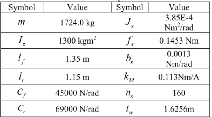
_current is a conversion from units of torque (N-m) to current (A).

Table 1 Vehicle parameters

Symbol Value Symbol Value

m

1724.0 kg

J

_s _Nm3.85E-4 2_/rad z

I

1300 kgm2 s

f

0.1453 Nm f

l

1.35 m

b

_s _Nm/rad0.0013 r

l

1.15 m

k

_M 0.113Nm/A f C 45000 N/rad

n

_s 160 r C 69000 N/rad

t

_w 1.6256m

3.2 Vehicle Model Validation Using Test Data

Validation of the vehicle model is accomplished by comparison of simulation predictions to P1 test data obtained using P1’s GPS/INS sensor suite. The longitudinal velocity data is used as the reference input for a cruise controller that sends voltage commands to the traction system model. The mean of the left and right steering angles from the test data is used as the reference input for the steering system model. Fig. 3 shows a comparison of test data and simulation results.

0 5 10 15 20 25 30 35 40 -12 -6 0 6 12 18 Test Data Vehicle Model Ste er ing A ngl e[ deg] Time [sec]

(3)

0 5 10 15 20 25 30 35 40 24 30 36 42 Test Data Vehicle Model Vehi cl e Speed [kph ] 0 5 10 15 20 25 30 35 40 -40 -20 0 20 40 Test Data Vehicle Model Ya w Ra te [de g/ s] 0 5 10 15 20 25 30 35 40 -8 -4 0 4 8 12 Test Data Vehicle Model Latera l Ac cel [m/s 2] Time [sec]

Fig. 3. Comparison of test data and vehicle simulation results The simulation predictions agree closely with the test data, suggesting that the model is feasible as a test platform for development of the steering and speed controllers in the linear handling regime of the test vehicle (Ha et. al., 2003)

4. DEVELOPMENT OF THE STEERING CONTROLLER FOR PATH-TRACKING

4.1 Control Objective

Fig. 4 shows the driver-vehicle system. In Fig.4, lateral position error (yr) is defined as the lateral distance between the vehicle C.G (C) and the centerline of the desired path (R). Yaw angle error (

ε ε

−

_d) is defined using the yaw angle of the vehicle (

ε

) and the desired yaw angle as dictated by the desired path (

ε

_d) (Kang et. al., 2006, 2007).

p L Gl ob a l X c oor d in a te

ε

r y d ε

Fig. 4. Driver –vehicle system

The rate of change of the lateral position error (yr) and yaw angle error (

ε ε

−

_d) are defined as in (6) and (7) (Peng, 1992), ( ) ( ) y y x d r y x d y v t v t y v v

ε ε

⋅ + ⋅ ⋅ − = + ⋅ −

(6) x , x d d v t v ε ε ρ ρ ⋅ = (7)

where

ρ

denotes the curvature radius of the desired path.

We seek to eliminate lateral and yaw angle error through a combination of feedback and feed-forward control. The feedback control input of the steering controller for path-tracking is computed using lateral position error and yaw angle error. The feed-forward control input is computed using the road information within the preview distance. To develop the steering controller using finite preview control theory, preview distance is transformed into preview time (Tp) as in (8). p p x L T v = (8) 4.2 State Equation

A 2-DOF bicycle model is used to design the steering controller. Equation (9) shows the dynamic equations for a 2-DOF bicycle model,

( ) y x yf yr z f yf r yr m v m v F F I l F l F ε ε ⋅ + ⋅ ⋅ = + ⋅ = ⋅ − ⋅

(9)

where m denotes the mass of the body,

I

_z the yaw moment of inertia, F_yf and F_yr the front and rear lateral tire force, and l_f and l_r the distance from the center of gravity(CG) to the front and rear axles, respectively. From the linear tire model, the lateral tire forces can be expressed as shown in (10), ( ) ( ) { ( ) } y f yfl yfr f f x r f d f f f d d x x v l F F C v y l l C v v ε δ ε ε δ ε ε ε + ⋅ = = ⋅ − + ⋅ − = ⋅ − + − − ⋅ (10) ( ) ( ) { ( ) } y r yrl yrr r x r r d r r d d x x v l F F C v y l l C v v ε ε ε _{ε ε} _ε − ⋅ = = ⋅ − − ⋅ − = ⋅ − + − + ⋅

where C_f and C_r denote the equivalent front and rear

cornering stiffnesses. Substituting (10) into (9), the state equations can be obtained as in (11) _{(Peng et. al., 1990),}

[ ] f d d T r r d d x A x B F w x y y

δ

ε ε

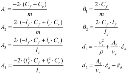
= ⋅ + ⋅ + ⋅ = − − (11) where 1 2 1 3 4 3 0 1 0 0 0 0 0 0 1 0 x x x x A A A v v A A A A v v ⎡ ⎤ ⎢ ⎥ ⎢ − ⎥ ⎢ ⎥ = ⎢ ⎥ ⎢ ⎥ ⎢ ⎥ − ⎢ ⎥ ⎣ ⎦ ₁ 2 0 0 B B B ⎡ ⎤ ⎢ ⎥ ⎢ ⎥ = ⎢ ⎥ ⎢ ⎥ ⎣ ⎦ 0 0_{1 0} 0 0 0 1 d F ⎡ ⎤ ⎢ ⎥ ⎢ ⎥ = ⎢ ⎥ ⎢ ⎥ ⎣ ⎦ 1 2 d d w d ⎡ ⎤ = ⎢ ⎥ ⎣ ⎦

(4)

1 2 3 2 2 4 2 ( ) 2 ( ) 2 ( ) 2 ( ) f r f f r r f f r r z f f r r z C C A m l C l C A m l C l C A I l C l C A I − ⋅ + = ⋅ − ⋅ + ⋅ = ⋅ − ⋅ + ⋅ = − ⋅ ⋅ + ⋅ = 1 2 2 2 1 4 2 2 2 f f f z x d x d d x C B m C l B I v A d v A d v ε ρ ε ε ⋅ = ⋅ ⋅ = = − + ⋅ = ⋅ −

In (11), the disturbance term (

w

_d) is defined from road

information (

ε

_d,

ε

_d).

4.3 Steering Controller Using Finite Preview Optimal Control Theory

The steering control input(

δ

f( )t ) is computed to minimize

the performance index given in (12) (Chen, 1988).

0 1 ( ) 1 lim { 2 } ( ) f f t T T f f t _T f f d d x Qx R E dt t _{A x B} _{F w} _x δ δ λ δ →∞ ⎡ ₊ ₊ ⎤ ⎢ ⎥ ⎢ _⋅ _{⋅ + ⋅} ₊ _⋅ ₋ ⎥ ⎢ ⎥ ⎣ ⎦

∫

(12)

The solution that minimizes the performance index is given by the well-known Euler Lagrange equation:

1 ( ) ( , , ) 2 ( )] T T f f T f d d x Qx R L x t A x B F w x δ δ λ λ δ ⎡ _⋅ ₊ ₊ ⎤ ⎢ ⎥ = ⎢ ⎥ ⋅ ⋅ + ⋅ + ⋅ − ⎢ ⎥ ⎣ ⎦ (13) i) L d L ₀ _{Qx A}T x dt x λ λ ∂ ₋ ⎡∂ ⎤₌ _⇒ _{= −} ₋ ⎢ ⎥ ∂ ⎣∂ ⎦ (14) ii) ₀ 1 T f f f L d L _{R B} dt δ λ δ δ − ⎡ ⎤ ∂ ₋ ∂ ₌ _⇒ _{= −} ⎢ ⎥ ∂ _⎢_⎣∂ _⎥_⎦ (15) iii) ₀ 1 T d d L d L x Ax BR B F w dt λ λ λ − ∂ ₋ ⎡∂ ⎤_{= ⇒ =} ₋ ₊ ⎢ ⎥ ∂ ⎣∂ ⎦ (16)

In order to obtain solutions for x t( ),

λ

( )t and

δ

f( )t ,

λ

( )t

is assumed to take the form shown in (17)

(

Burl, 1998). ( )t P t x t( ) ( ) H t( )

λ = + (17) where H t( )is a feed-forward control. The differential form of (17) is shown below: 1 [ ] ( ) [ ( )] T d d T Px P Ax BR B F w H t Qx A Px H t λ₌ _{+ ⋅} ₋ − λ₊ ₊ = − − ⋅ + (18)

Substituting (17) into (18) and grouping terms, the following two equality conditions are obtained (Chen, 1988)

1 T T ₀ P PA PBR B P A P Q₊ ₋ − ₊ _{+ =} ₍₁₉₎ T c d d

H

= −

A H P F w

⋅ − ⋅

⋅

(20) where 1 T c

A

= − ⋅

A B R

−

⋅

B P

⋅

Equation (19) is the standard LQ Riccati equation. As

t

→ ∞

, the solution ( )P t of (19) tends to approach its steady state value and is independent of the final condition

( )f

P t . Then, equation (19) becomes the well-known Control

Algebraic Riccati Equation as shown below:

1 T T ₀

ss ss ss ss

P A P BR B P₋ − ₊A P _{+ =}Q ₍₂₁₎

If the road information beyond the preview time (Tp) is set equal to zero ( w t_d( ) 0= , ∀ ∈ + ∞t t T[ _p, ]), equation (20) becomes (Chen, 1988): ( ) ( , ) [ ( )] p T c t T A t p ss d d t H t T e τ P F w τ dτ + − − =

_∫

⋅ ⋅ ⋅ (22)

As a result, the steering control input is computed as in (23),

( ) ( ) ( ) desired t Kopt x t M t

δ

= − ⋅ + (23) where 1 T opt ss K _{= −}R− _⋅B P_⋅ _, 1

( )

T c A t ss d

F t

=

e

⋅

P F

⋅

1 1 0 ( ) ( ) ( ) p T T M t _{= −}R− _⋅B _⋅ F ξ _⋅w t_{+ ⋅}ξ dξ

∫

From (23), it is clear that the steering control input is computed using the road information between t and t+Tp. Fig. 5 shows the block diagram for the steering controller.

r r d d y y x ε ε ε ε ⎡ ⎤ ⎢ ⎥ ⎢ ⎥ =_⎢ _⎥ − ⎢ ₋ ⎥ ⎣ ⎦ ff δ fb δ desired δ Road Information

Between t and t+Tp Disturbance Computation

( ) opt K x t − ⋅ ∑ p p x T L N N v ξ Δ = = ⋅ Vehicle Speed 1 1 0 [ ( ) ( ) ] N T i R B− Fξ w t i ξ ξ = − ⋅ ⋅∑ ⋅ + ⋅Δ ⋅Δ ( ) i w w t i= + ⋅Δξ

Fig. 5. Block diagram of steering controller

The desired steering angle which is computed by the steering controller is applied to the vehicle model and test vehicle using Ackermann steering geometry as in (24),

1 ( / 2 ) desired fL desired tw L δ δ δ = − ⋅ ⋅ (24) 1 ( / 2 ) desired fR desired tw L δ δ δ = + ⋅ ⋅

where

δ

_fL and

δ

_fR denote the left and right front steering angle, respectively, and

L

the wheelbase.

5. DEVELOPMENT OF THE SPEED CONTROLLER The speed controller is designed to create safe lateral vehicle behavior by means of keeping the lateral acceleration below a critical value (a_y_{_ limit}) as follows,

Limit Limit Set desired

Set Limit Set

V if V V V V if V V ≤ ⎧ = ⎨ _> ⎩ (25) 2 2 _ limit _ limit x Limit y y Limit y V V a a V ρ a ρ ≤ ρ ≤ ⇒ = ⋅

(5)

where,

V

_set the vehicle set speed determined by the driver, and V_Limit the vehicle speed required to not exceed a_y_{_ limit}. In order to track the desired speed, the speed command (voltage sent to the drive motors) is computed using the proportional controller as shown below

x V Limit V Set V Vdesired

Fig. 6. Block diagram of Speed Controller

( )

driving motor cruise x desired

V =K ⋅ V −V (26)

where K_cruise denotes the cruise control proportional gain. 6. SIMULATION RESULTS

Simulations have been run with the steering controller active at constant speed and when the speed controller is integrated with the steering controller as shown below.

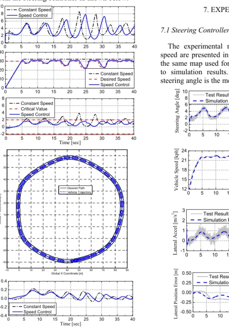
0 5 10 15 20 25 30 35 40 0 2 4 6 8 10 Constant Speed Speed Control S teeri ng Ang le[ deg] 0 5 10 15 20 25 30 35 40 0 10 20 30 40 Constant Speed Desired Speed Speed Control Vehicle Speed [kph] 0 5 10 15 20 25 30 35 40 -2 0 2 4 6 8 Constant Speed Critical Value Speed Control La ter al A cc el [m/s 2] Time [sec] -10 0 10 20 30 40 50 60 70 80 90 -30 -20 -10 0 10 20 30 40 50 60 Global X Coordinate [m] G lob al Y Co or di na te [m ] Desired Path Vehicle Trajectory 0 5 10 15 20 25 30 35 40 -0.4 -0.2 0.0 0.2 0.4 Constant Speed Speed Control L ateral Position Err or [m ] Time [sec] 0 5 10 15 20 25 30 35 40 -4 -2 0 2 4 Constant Speed Speed Control Yaw Ang le Error [deg ] Time [sec]

Fig. 7. Simulation results for steering controller and integrated controller

The simulations use a map located at a parking lot at Stanford University. Fig. 7 compares the simulation results under the two test scenarios. In both scenarios, the vehicle tracks the map very closely, with the magnitude of lateral and yaw angle errors not exceeding 0.2 m and 1 deg, respectively. The simulation results also show that the lateral acceleration of vehicle doesn’t exceed a_y_{_ limit} during path tracking with the speed controller active. Also, the lateral acceleration is lower magnitude when compared to path tracking at the constant (set) speed. As a result, it is found that the safety of lateral vehicle behavior is improved with the speed controller active in conjunction with the steering controller.

7. EXPERIMENTAL RESULTS

7.1 Steering Controller at Constant Speed

The experimental results for path tracking at constant speed are presented in Fig.8. The tests were performed with the same map used for simulation studies, and are compared to simulation results. In Figs.8 and 9, the experimental steering angle is the mean of the left and right steering angles.

0 5 10 15 20 25 30 35 40 45 50 -2 0 2 4 6 8 10 Test Result Simulation Result St ee ri ng A ng le [d eg ]

120 5 10 15 20 25 30 35 40 45 50 15 18 21 24 Test Result Simulation Result Veh icl e S pee d [k ph ]

0 5 10 15 20 25 30 35 40 45 50 -1 0 1 2 3 Test Result Simulation Result Lat eral A ccel [ m /s 2 ]

0 5 10 15 20 25 30 35 40 45 50 -0.50 -0.25 0.00 0.25 0.50 Test Result Simulation Result Lateral Posi tion Error [m] Time [sec]

(6)

0 5 10 15 20 25 30 35 40 45 50 -2 -1 0 1 2 Test Result Simulation Result Ya w Ang le Error [ m ] Time [sec]

Fig. 8. Comparison of the simulation results and test results, constant speed test

The test results agree closely with the simulation results. The steering controller produces satisfactory tracking performance, with the magnitudes of lateral and yaw angle error below 0.25 m and 1.5 degrees, respectively. These errors are on the same order of magnitude as the errors predicted in simulation.

7.2 Steering Controller Integrated With Speed Controller

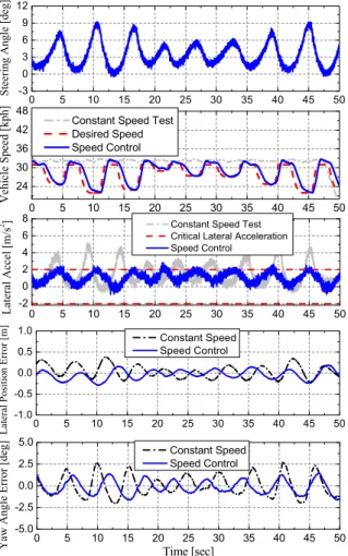
The test results for the integrated controllers are presented in Fig. 9 and compared with test results at a constant speed equivalent to the set speed for the speed controller:

0 5 10 15 20 25 30 35 40 45 50 -3 0 3 6 9 12 Stee rin g An gle [d eg ] 0 5 10 15 20 25 30 35 40 45 50 24 30 36 42 48

Constant Speed Test Desired Speed Speed Control V ehi cle Sp eed [kp h] 0 5 10 15 20 25 30 35 40 45 50 -2 0 2 4 6

8 _{Constant Speed Test}

Critical Lateral Acceleration Speed Control Late ral Acce l [m /s 2 ] 0 5 10 15 20 25 30 35 40 45 50 -1.0 -0.5 0.0 0.5 1.0 Constant Speed Speed Control Lat eral P ositio n Err or [m ] 0 5 10 15 20 25 30 35 40 45 50 -5.0 -2.5 0.0 2.5 5.0 Constant Speed Speed Control Y aw An

gle Error [deg]

Time [sec]

Fig. 9. Comparison of test results, constant speed test versus test with integrated controller

The “bulk” acceleration of the vehicle (neglecting high frequency variation due to vibration, wheel hop, etc.) is maintained below the lateral acceleration limit of 2 m/s2_{. As} predicted in simulation, use of the speed controller in conjunction with the steering controller significantly reduces

lateral acceleration when compared to path-tracking at the constant (set) speed.

8. CONCLUSIONS

A steering controller integrated with a speed controller for autonomous vehicle path tracking has been presented in this paper. The controllers were developed using a numerical simulation study and implemented on a by-wire test vehicle. From the simulation results and the test results, it is found that the steering controller using finite preview optimal control produces satisfactory path tracking performance. Furthermore, the safety of lateral vehicle behaviour is improved by combining the steering controller with a speed controller that maintains a lateral acceleration limit.

ACKNOWLEDGMENTS

This work has been supported by BK21 School for Creative Engineering Design of Next Generation Mechanical and Aerospace Systems, Korea.

REFERENCES

Burl, Jeffrey B. (1998). Linear Optimal Control, pp.179~226. Addison-Wesley Longman, Boston, MA.

Chen, Long-Chain (1988). An active suspension system with preview control for passenger automobiles. PhD Thesis,

Massachusetts Institute of Technology.

Gadda, Christopher D., Shad M. Laws, and J. Christian Gerdes (2007), Generating Diagnostic Residuals for Steer-by

Wire Vehicles. IEEE Transactions on Control Systems

Technology, Vol. 15, No. 3, pp. 529~540. Ha, Jungsoo (2003). Validation of 3D Vehicle Model and

Driver Steering Model with Vehicle Test. Spring Conf. Proc. KSAE, Vol. 2, pp. 676-681.

Hess, R.A., A. Modjtahedzadeh (1990). A Control theoretic model of driver steering behaviour. IEEE control Systems Magazine, Vol. 10, No. 5, pp. 3~8. Peng, Huei (1992). Vehicle Lateral Control for Highway Automation. PhD Thesis, University of California at Berkeley.

Peng, H., Tomizuka, M. (1990), Lateral Control of Front-Wheel-Steering. Rubber-Tire Vehicles, Publication of PATH project, ITS, UC Berkeley, UCB-ITS-PRR-90-5 Ryu, Jihan and J. Christian Gerdes (2004). Integrating Inertial

Sensors with GPS for Vehicle Dynamics Control.

Journal of Dynamic Systems, Measurement and Control, Vol. 126, pp. 243-254.

Kang, JuYong., Yi, Kyongsu. and Noh, Kihan. (2006), Development of a Finite Preview Optimal Control-based Human Driver Steering Model, KSAE Spring Conference in 2006, KSAE, Vol. III, pp. 1632~1637 Kang, JuYong., Yi, Kyongsu. and Noh, Kihan. (2007),

Development and Validation of a Finite Preview Optimal Control-based Human Driver Steering Model,

KSME Spring Conference in 2007, KSME, pp. 130~135 Kim, Wongun. and Yi, Kyongsu. (2007), Development of an

InTelligent Autonomous Control Algorithm and Test Vehicle Performance Verification, KSME Spring Conference in 2007, KSME, pp. 136~141