Analysis of the Dynamics and Microphysics of a Wet Downburst Case Using Dual-Polarization Radar Data

(1)

UNIVERSITY OF OKLAHOMA GRADUATE COLLEGE

ANALYSIS OF THE DYNAMICS AND MICROPHYSICS OF A WET DOWNBURST CASE USING DUAL-POLARIZATION RADAR DATA

A DISSERTATION

SUBMITTED TO THE GRADUATE FACULTY in partial fulfillment of the requirements for the

Degree of

DOCTOR OF PHILOSOPHY

By

VIVEK NARAYAN MAHALE Norman, Oklahoma

(2)

ANALYSIS OF THE DYNAMICS AND MICROPHYSICS OF A WET DOWNBURST CASE USING DUAL-POLARIZATION RADAR DATA

A DISSERTATION APPROVED FOR THE SCHOOL OF METEOROLOGY

BY

Dr. Guifu Zhang, Chair Dr. Ming Xue, Co-Chair Dr. Howard Bluestein Dr. Youngsun Jung Dr. Yan Zhang

(3)

(4)

iv

This dissertation is dedicated to my parents, Narayan and Hema Mahale, and brother, Dilip.

(5)

v

Acknowledgements

It was 25 years ago (25 April 1994) that I became interested in meteorology when a tornado went through my neighborhood in DeSoto, Texas. Ever since then, I’ve been fascinated by the weather. I feel incredibly fortunate that I was able to study severe storms as this dissertation is a culmination of nearly a lifetime of interest. Without the support of family, friends, teachers, professors, colleagues, administrative assistants, and others this achievement would not be possible!

First and foremost, I would like to thank my advisors, Drs. Guifu Zhang and Ming Xue, for their support during my doctoral research. Their commitment through the countless hours they spent on providing guidance, attending meetings, reviewing manuscripts, etc. cannot be overstated. I also appreciate their patience to work around my shiftwork at the National Weather Service (NWS). I also wish to thank my committee members Dr. Howard Bluestein, Dr. Youngsun Jung, Dr. Yan Zhang, and former member, Dr. Jerry Brotzge, for taking the time to serve on my committee. I am especially thankful for Drs. Howard Bluestein and Jerry Bortzge for serving as advisors during my master’s degree. They set the foundation for my success in the doctoral program!

I am also grateful for Jeff Snyder and Andrew Pazmany for collecting the RaXPol data used in this dissertation. Jeff Snyder also provided technical assistance in the installation and use of radar analysis software. I am also appreciative of Robin Tanamachi for providing insight, photography, and video of the downburst event. Jidong Gao and Heather Reeves provided feedback to significantly improve the chapter on the variational retrieval method.

Also, thank you to the administrative assistants and staff of the School of Meteorology (SoM), Advanced Radar Research Center (ARRC), and Center for Analysis and Prediction of

(6)

vi

Storms (CAPS) that have provided support over the last several years. Debbie Barnhill, Krysta Bruehl, Nancy Campbell, Debra Farmer, Eileen Hasselwander, Ashley Hill, Celia Jones, Jo Ann Mehl, Marcia Pallutto, Becky Steely, Christie Upchurch, and Lauren White all provided some assistance over the last several years.

I am appreciative of all my friends and colleagues that I met while at SoM. Several fellow (former) classmates are close friends, and I want thank all of them for their friendship through my undergraduate and/or graduate school career. Not only did we work hard to succeed in classes and research together, but we also had some awesome and memorable times outside of school. Daniel Betten, Tim Bonin, Brandon Lawson, Jim Kurdzo, Jennifer Newman, Bryan Putnam, Brett Roberts, Chris Schwarz, and Derek Stratman have all been great friends over the last several years! Other supportive colleagues are my former officemates: Jana Houser, Mike French, Dylan Reif, Kyle Thiem, and Zach Wienhoff.

I also appreciate the strong support I received from the NWS Norman, Oklahoma, management and staff. David Andra (MIC), Rick Smith (WCM), and Todd Lindley (SOO) have been supportive in my goal to finish my doctoral degree while working fulltime as a shift worker at the NWS. I am appreciative of my coworkers’ flexibility to allow me to attend advisor meetings and conduct research during some quiet weather days. Marc Austin, Ryan Barnes, Randy Bowers, Kevin Brown, Scott Curl, Matthew Day, Jon Kurtz, Erin Maxwell, Forrest Mitchell, John Pike, Wayne Ruff, Michael Scotten, Cheryl Sharpe, Doug Speheger, Jennifer Thompson, Bruce Thoren, Phil Ware, and Alex Zwink have all been incredibly supportive colleagues! I also appreciate the strong support from Jami Boettcher, Mike Foster, Suzanne Jenkins, and Chris Sohl from my NWS family (some of whom have retired).

(7)

vii

I would also like to thank professors and teachers in my past that provided the foundation necessary for me to be successful in my educational endeavors. Many of these individuals encouraged me to study meteorology because of my passion for it. It would be impossible for me to name every teacher, but Mike Carney and Bryan Yockers played an important role as my AP Environmental Science and AP Physics teachers at Jenks High School. They have both been extremely supportive from high school to the present. Mr. Carney even found me an opportunity to job shadow at the NWS in Tulsa, Oklahoma, my junior year of high school, which I am grateful for!

Finally, the love and support of my family has been unwavering and cannot be overstated. My parents, Narayan and Hema Mahale, and my brother, Dilip, have been supportive in many ways and it would be difficult to list everything they have done for me. The bottom line—without them, I would not be where I am today!

Financial support during the early part of this research came from NSF grant AGS-1046171, "Advanced Study of Precipitation Microphysics with Multi-frequency Polarimetric Radar Observations and Data Assimilation".

Substantial portions of this dissertation are from three of my lead-author publications that are either published, conditionally accepted, or in-preparation:

Mahale, V. N., G. Zhang, and M. Xue, 2016: Characterization of the 14 June 2011 Norman, Oklahoma, downburst through dual-polarization radar observations and hydrometeor classification. J. Appl. Meteor. Clim., 55, 2635–2655.

Mahale, V. N., G. Zhang, M. Xue, J. Gao, and H. D. Reeves, 2019: Variational retrieval of rain microphysics and related parameters from polarimetric radar data with a parameterized operator. J. Atmos. Oceanic Technol., conditionally accepted.

(8)

viii

Mahale, V. N., G. Zhang, M. Xue, H. B. Bluestein, and J. C. Snyder, 2019: Rapid-scan dual- polarization radar observations of the 14 June 2011 Norman, Oklahoma, downburst and associated gust front and rotor, in-preparation.1

The publication(s) that correspond to each chapter are acknowledged as a footnote at the beginning of each chapter. The publication in the Journal of Applied Meteorology and Climatology is © Copyright 2016 American Meteorological Society (AMS). Additional details (including the full copyright notice) are provided in the AMS Copyright Policy statement, available on the AMS website (http://www.ametsoc.org/CopyrightInformation). The AMS grants permission to use any portion of the author’s work in works of the author's own, provided that the AMS citation and notice of the AMS copyright are included.

1

(9)

ix

List of Figures

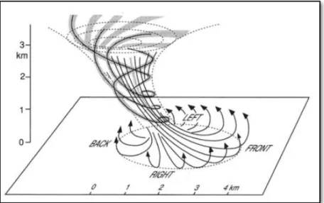
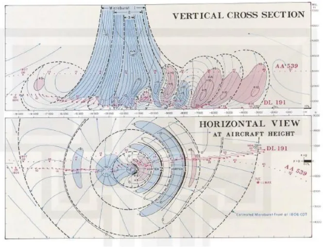
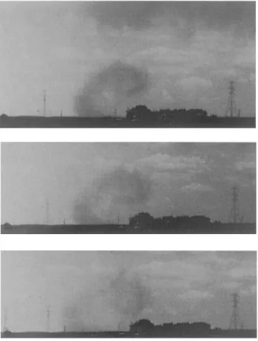
Fig. 2.1. A painting of a downburst based on Fujita’s sketches of the downburst associated with the 1985 of Delta Flight 191 at the Dallas-Fort Worth (Texas) airport. From Fujita (1986). ... 4 Fig. 2.2. Schematic diagram illustrating the impact of a downburst on an aircraft’s performance during takeoff. The aircraft first encounters a headwind during takeoff, which results in enhanced lift. This is followed by a decreasing headwind component, a downdraft, and finally a strong tailwind. Overcompensation during the period of enhanced lift may result in stalling and an impact with the ground. Composite drawing based on numerous studies of aircraft accidents by Fujita and Caracena (1977), Fujita and Byers (1977), and Fujita (1978, 1985, 1986). From (Wakimoto 2001). ... 5 Fig. 2.3. Three-dimensional visualization of a downburst. From Wakimoto (2001), which was adapted from Fujita (1985). ... 7 Fig. 2.4. A vertical cross section and horizontal view of the Delta Flight 191 microburst at 1806 CDT on August 2, 1985. This microburst, approximately 16,000’ (3.5 km or 1.9 n.m.) in diameter, is characterized by three major Vortices 1, 2, and 3, which are surrounded by an older vortex encircling the overall microburst. From Fujita (1986). ... 8 Fig. 2.5. A sequence of photos showing the curling features of dust clouds (i.e., rotors or horizontal vortices) behind the leading edge of a microburst outflow on 15 July 1982 during the JAWS field operation. Photos by Brian Waranauskas. From Fujita (1985). ... 9 Fig. 2.6. Schematic of a vertical cross section through a mature thunderstorm outflow. From Droegemeier and Wilhelmson (1987); based on previous work from Charba (1974), Goff (1976), Wakimoto (1982), and Koch (1984). ... 10

(13)

xiii

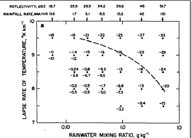
Fig. 2.7. Results of a one-dimensional time dependent nonhydrostatic cloud model of a downdraft. Plotted numbers are vertical air velocity (m s-1) at a level 3.7 km below the top of the downdraft (~850 hPa) as a function of the lapse rate in the environment and total liquid water mixing ratio at the top of the downdraft. Numbers on top scale indicate the radar reflectivity and rain rate at the top of the downdraft. Curved dotted line separates downbursts (<20 m s-1) from less intense downdrafts. It was found that as the environmental lapse rate decreases (increases), higher (lower) water content is needed for a downburst. From Srivastava (1985). ... 15 Fig. 2.8. Horizontal radar reflectivity factor (ZH) and radial velocity (VR) from KOUN on 15 June 2011 at 0022 UTC. The characteristic low-level radial divergence signature associated with the downburst is seen. Plotted using GR2Analyst. ... 17 Fig. 2.9. Vertical cross section showing dual-polarization Doppler radar measurements obtained in a thunderstorm in northern Alabama during the MIST project. Note the presence of a ZDR hole within the main precipitation core within a microburst-producing downdraft, which indicates the presence of melting hail. Reflectivity data are presented in contours of dBZ. ZDR are shown in dB units. Arrow indicates location of the center of a surface microburst. From Wakimoto and Bringi (1988). ... 18 Fig. 3.1. Photo of RaXPol collecting data from the downburst in Norman, Oklahoma, on 14 June 2011. Note that the wet downburst is seen in the background. Photo courtesy Robin Tanamachi. ... 23 Fig. 3.2. Map of RaXPol, KOUN, and the Norman, Oklahoma, Mesonet locations during data collection. KOUN was located approximately 256 m to the southeast of RaXPol. The Norman Mesonet station was located approximately 221 m to the southwest of RaXPol. Plotted using Google Earth. ... 24

(14)

xiv

Fig. 4.1. Official storm reports and event narrative for the Norman, Oklahoma, downburst from the National Centers for Environmental Information (NCEI) Storm Events Database. The table abbreviations are: St. is state; T.Z. is time zone; Mag is magnitude; Dth is deaths; Inj is injuries; PrD is property damage estimate; and CrD is crop damage estimate. From NOAA/NCDC (2011). ... 26 Fig. 4.2. Map of wind damage reports (courtesy National Weather Service Norman, Oklahoma), (b) photo of the downburst from north Norman, and (c) photo of damage at Max Westheimer Airport. Photos courtesy Robin Tanamachi. ... 27 Fig. 4.3. Upper-air sounding and hodograph from Norman, Oklahoma (KOUN) at 0000 UTC 15 June 2011. Temperature is denoted by the red line and dew point by the green line. The purple line is the virtual temperature correction, and the turquoise line represents the parcel path for surface-based parcel. Plotted using The Universal Rawinsonde Observation (RAOB) program. ... 29 Fig. 4.4. KTLX radar reflectivity (dBZ) and Oklahoma Mesonet surface observations valid at (a) 2315, (b) 2345, and (c) 0005 UTC. Surface temperature (°C), dew point (°C), and wind barbs (full barb ≡ 5 m s-1_{; half barb ≡ 2.5 m s}-1

) are plotted. The white circle highlights the storm that would produce the downburst. The dashed blue line is the approximate location of the cold front. The location of the Norman and Minco Mesonet stations are indicated. Plotted using WeatherScope from the Oklahoma Climate Survey. ... 31 Fig. 4.5. 1-min Oklahoma Mesonet data at Norman, Oklahoma, of (a) surface pressure (hPa) and rain rate (mm hr-1), (b) 2 m temperature (°C) and 2 m relative humidity (%), and (c) 10 m maximum wind gust (m s-1) and wind direction (degrees) valid from 2330 to 0130 UTC. The

(15)

xv

times of the gust front passage, downburst start, and downburst end are noted by the dashed lines. ... 33 Fig. 4.6. Time evolution of surface observations as the downburst passed over the Oklahoma Mesonet station at Norman, Oklahoma. Time relative maximum and minimum surface pressure are noted by “H” and “L”, respectively. Gust front passage is noted by cold front symbol. Schematic is based upon 1-min data from Figure 4.5. ... 36 Fig. 5.1. Reconstructed range height indicator (RHI) analyses from KOUN. Horizontal radar reflectivity factor (ZH), co-polar correlation coefficient (ρhv), and differential reflectivity (ZDR) are shown at (a) 2333-2337 UTC, (b) 2338-2342 UTC, (c) 2243-2347 UTC, and (d) 2348-2352 UTC volume scans. Axes are labeled relative to KOUN. RHI azimuth angle and noteworthy storm features are denoted. ... 43 Fig. 5.2. Reconstructed range height indicator (RHI) analyses from KOUN. Radial velocity (VR) and hydrometeor classification algorithm (HCA) are shown at (a) 2333-2337 UTC, (b) 2338-2342 UTC, (c) 2243-2347 UTC, and (d) 2348-2352 UTC volume scans. The classifications on the right panel are: 1) ground clutter and anomalous propagation (GC/AP); 2) biological scatterers (BS); 3) dry aggregated snow (DS); 4) wet snow (WS); 5) crystals (CR); 6) graupel (GR); 7) big drops (BD); 8) light and moderate rain (RA); 9) heavy rain (HR); and 10) a mixture of rain and hail (RH). Axes are labeled relative to KOUN. RHI azimuth angle and noteworthy storm features are denoted. ... 44 Fig. 5.3. Same panels as Figure 5.1, but at (a) 2353-2357 UTC, (b) 2358-0002 UTC, (c) 0003-0007 UTC, and (d) 0008-0012 UTC volume scans. ... 46 Fig. 5.4. Same panels as Figure 5.2, but at (a) 2353-2357 UTC, (b) 2358-0002 UTC, (c) 0003-0007 UTC, and (d) 0008-0012 UTC volume scans. ... 47

(16)

xvi

Fig. 5.5. Same panels as Figure 5.1, but at (a) 0013-0017 UTC, (b) 0018-0022 UTC, and (c) 0023-0027 UTC volume scans... 50 Fig. 5.6. Same panels as Figure 5.2, but at (a) 0013-0017 UTC, (b) 0018-0022 UTC, and (c) 0023-0027 UTC volume scans... 51 Fig. 5.7. Dual-Doppler analysis at (a) 0018 UTC and (b) 0023 UTC with KOUN 1.45° radar reflectivity and hydrometeor classification algorithm (HCA). Dual-Doppler analysis includes horizontal velocity vectors and vertical velocity contours. Contours are plotted in 5 m s-1 intervals in white on the radar reflectivity panels and in black on the HCA panels. The location of Newcastle, Oklahoma, is indicated on panel (a). ... 54 Fig. 5.8. Schematics of the microphysical evolution of hydrometeors during the Norman, Oklahoma, downburst as observed by polarimetric radar data (PRD) and the applied hydrometeor classification algorithm (HCA). The schematics depict raindrops, snow, graupel, hail, and melting hail. Increasing water coating on the melting hailstones is depicted by the increasing line width of the hailstones. The 0 °C level is depicted by the dotted yellow line. Local ZDR maxima (e.g., ZDR columns) are depicted by the dashed red line. Local ZDR minima are depicted by the dashed green line. The updraft and downburst locations are depicted by the green and blue arrows, respectively. Shaded blue region represents the cold pool. It is assumed that diabatic cooling from hail melting and rain evaporation plays an important role in accelerating the downdraft to result in a downburst. ... 58 Fig. 6.1. Horizontal radar reflectivity (ZH; dBZ), radial velocity (VR; m s-1), and co-polar correlation coefficient (ρhv) at 3.0° elevation angle are shown at (a) 0018:50 UTC and (b) 0020:29 UTC. The dotted line (white on VR; black on ZH and ρhv) is the distance between the maximum inbound velocity on the southeastern part of the storm and the maximum outbound

(17)

xvii

velocity on the northern part of the storm. 1 km range rings and axes are labeled relative to RaXPol’s location. ... 63 Fig. 6.2. Same panels as Figure 6.1, but 3.0° elevation angle at (a) 0022:07 UTC and (b) 0023:45 UTC... 65 Fig. 6.3. 0023:45 UTC horizontal radar reflectivity (ZH; dBZ), radial velocity (VR; m s-1), spectrum width (σv; m s-1), differential reflectivity (ZDR; dB), co-polar correlation coefficient (ρhv) and differential phase (ϕDP; degrees) at 3.0° elevation angle. Vertical vortices are circled in black. 1 km range rings and axes are labeled relative to RaXPol’s location. ... 67 Fig. 6.4. Same panels as Figure 2, but 3.0° elevation angle at (a) 0025:23 UTC and (b) 0027:01 UTC... 69 Fig. 6.5. The downburst’s spatiotemporal evolution between 0020:29 and 0027:01 UTC. The downburst’s horizontal scale is shown with respect to time and maximum inbound radial velocity (Vr). The downburst grew in horizontal scale from at least 2.1 km to 6.4 km in less than 7 min, changing based on size from a microburst to a macroburst while intensifying. ... 71 Fig. 6.6. Reconstructed range height indicator (RHI) from RaXPol at ~310° azimuth. Horizontal radar reflectivity (ZH; dBZ), radial velocity (m s-1), and co-polar correlation coefficient (ρhv) volume scans are shown at (a) 0018:50-0020:16 UTC and (b) 0020:29-0021:54 UTC. Axes are labeled relative to RaXPol’s location. Noteworthy storm features are denoted. ... 73 Fig. 6.7. Same panels as Figure 6.5, but volume scans at (a) 0022:07-0023:32 UTC and (b) 0023:45-0025:10 UTC. ... 75 Fig. 6.8. Same panels as Figure 6.5, but volume scans at (a) 0025:23-0026:48 UTC, (b) 0027:01-0028:26 UTC, and (c) 0028:40-0030:05 UTC. ... 78

(18)

xviii

Fig. 6.9. 1-min Oklahoma Mesonet data at Norman, Oklahoma, of (a) 10 m maximum wind gust (m s-1) and wind direction (degrees) and (b) surface pressure (hPa) and 2 m temperature (°C) from 0016 to 0030 UTC. The times of the 3.0° elevation angle scans are noted (red dotted line). ... 81 Fig. 7.1. Attenuation (AH: left column) and differential attenuation (ADP: right column) versus specific differential phase for (a, b) S-band and (c, d) X-band. Modified from Zhang (2016). ... 87 Fig. 7.2. Backscattering phase differences (δ) as a function of raindrop size at S-band, C-band, and X-band frequencies. Modified from Zhang (2016). ... 87 Fig. 7.3. ρhv as a function of mass/volume-weighted diameter of wet hail and fractional water content (𝑓𝑤) at (a) S-band (b) X-band and (c) S-band – X-band. These were calculated using the T-matrix method assuming an exponential PSD and with the canting angle as a function of𝑓𝑤. 90 Fig. 7.4. Flow chart describing the post-processing for PRD for KOUN and RaXPol to conduct dual-frequency comparisons between the two radars. ... 92 Fig. 7.5. Example of post-processing of ZH (dBZ) from a 5.3° elevation scan of KOUN WSR-88D data at 0020:08 UTC. (a) Pre-processed ZH, (b) ZH after the application of a median filter, (c) ZH after the application of a median filter and attenuation correction, (d) ZH after the application of a median filter, attenuation correction, and advection correction, and (e) ZH after the application of a median filter, attenuation correction, and advection correction interpolated to the RaXPol grid are shown. The grid spacing is 250 m x 1.1°. ... 94 Fig. 7.6. Example of post-processing of ρhv from a 5.0° elevation scan of RaXPol data at 0020:35 UTC. (a) Pre-processed ρhv and (b) ρhv downscaled from 75 m to 250 m range resolution. The grid spacing is 250 m x 1.1°. ... 94

(19)

xix

Fig. 7.7. Difference fields of KOUN- RaXPol radar data for (a) ZH, (b) ZDR, and (c) ρhv. Difference fields are calculated from the 5.3° elevation scan of KOUN WSR-88D data at 0020:08 UTC and 5.0° elevation scan of RaXPol data at 0020:35 UTC. The grid spacing is 250 m x 1.1°. ... 95 Fig. 7.8. HCA applied to 5.3° elevation scan of KOUN WSR-88D data at 0020:08 UTC. ... 96 Fig. 7.9. HCA results from Figure 7.8 plotted as a function of S-band ZH and ρhv difference between KOUN and RaXPol. ... 97 Fig. 8.1. The fitted parameterized polarimetric forward observation operators compared to direct calculations from T-matrix method for (a) Zh, (b) ZH, (c) Zdr, (d) ZDR, (e) KDP, and (f) ρhv. These are normalized for W of 1 g m-3. The equation on each panel is the derived observation operator. ... 106 Fig. 8.2. Block diagram of the iteration procedure for the nonlinear variational retrieval for a single azimuth of radar data. ... 112 Fig. 8.3. Analysis for (a) W and (b) Dm by applying the variational retrieval using a 5.3° elevation scan of KOUN WSR-88D data from 15 June 2011 at 0020 UTC. The boundaries of the sector with hail contamination are marked by the black lines. ... 113 Fig. 8.4. (a) ZH observations, (b) ZDR observations, (c) ZH analysis, (d) ZDR analysis, (e) ZH observations and analysis difference, and (f) ZDR observations and analysis difference using a 5.3° elevation scan of KOUN WSR-88D data from 15 June 2011 at 0020 UTC. The analyses are from applying the variational retrieval. ... 114 Fig. 8.5. KDP (a) calculated using the slope of a least squares fit and (b) from the variational retrieval using a 5.3° elevation scan of KOUN WSR-88D data from 15 June 2011 at 0020 UTC. The left panel was calculated using GR2Analyst software. The boundaries of the sector with hail

(20)

xx

contamination are marked by white lines on the left panel and black lines on the right panel. The area highlighted in yellow on the left panel is an area with some negative (unrealistic) KDP values. ... 115 Fig. 8.6. HCA applied to 5.3° elevation scan of KOUN WSR-88D data from 15 June 2011 at 0020 UTC. The boundaries of the sector with hail contamination are marked by the black lines. ... 116 Fig. 8.7. OI analysis and nonlinear analysis compared to the truth for (a) W, (b) ZH, (c) Dm, (d) ZDR, and (e) ΦDP using 2DVD data collected on 2005 May 13. The constant background field for W and Dm are also shown. ... 122 Fig. 8.8. Same panels as Figure 8.7, but with nonlinear analysis without ΦDP and nonlinear analysis with ΦDP compared to the truth. ... 124 Fig. 8.9. Same panels as Figure 8.7, but with nonlinear analysis without error and nonlinear analysis with random error compared to the truth. The simulated observation (truth + random error) for ZH, ZDR, and ΦDP are also shown. ... 126 Fig. 8.10. Analysis for (a) W, (b) ZH, (c) Dm, (d) ZDR, and (e) ΦDP by applying the variational retrieval on a single azimuth of 5.3° elevation scan of KOUN WSR-88D data from 15 June 2011 at 0020 UTC. The observed values for ZH, ZDR, and ΦDP are plotted for comparison. The empirical relationship and constant background field for W and Dm are shown as well. ... 129

(21)

xxi

Abstract

A significant, wet downburst affected Norman, Oklahoma, on 14 June 2011. Surface winds in excess of 35 m s-1 (>80 mph) and hailstones in excess of 4 cm diameter occurred during the downburst. The polarimetric S-band (~11.09-cm wavelength) KOUN Weather Surveillance Radar-1988 Doppler (WSR-88D) and the rapid-scan X-band (~3-cm wavelength) polarimetric, Doppler radar (RaXPol) collected nearly simultaneous polarimetric radar data (PRD) of the downburst.

The focus of this dissertation is the characterization and analysis of the dynamics and microphysics of the 14 June 2011 downburst and parent thunderstorm using various analysis methods. Analysis of the PRD from both KOUN and RaXPol radars are conducted using low-level plan position indicator (PPI) elevation scans and reconstructed range–height indicator (RHI) data. A hydrometeor classification algorithm (HCA) is applied to the KOUN PRD to understand the microphysical evolution of hydrometeors in the downburst. Dual-Doppler analysis is conducted with KOUN and the KTLX WSR-88D. Dual-frequency analysis and a comparison of the PRD are conducted between KOUN and RaXPol. Finally, a variational retrieval algorithm of rain microphysics is developed and applied to KOUN based on S-band parametrized polarimetric observation operators.

Through the above analyses, an understanding of the structure and evolution of the downburst and its potential driving mechanism(s) is developed. It is found that graupel aloft transitioned to nearly all rain and hail mixture above the 0 °C level. Eventually, this large area of rain and hail mixture (i.e., mixed-phase precipitation) descended to the ground with some melting of the hail, causing the downburst. The downburst grew from a microburst at ~2.1 km horizontal scale to a macroburst at ~6.4 km in less than 7 min. As the downburst expanded, its

(22)

xxii

near-surface horizontal winds intensified from 23 m s-1 to 42 m s-1. Descending surges of mixed-phase precipitation cores aloft, indicated by a reduction in co-polar correlation coefficient (ρhv), provided a continued stream of precipitation loading and melting hail that may have aided in the continued expansion and intensity of the downburst. The unique, rapid-scan observations also captured the development of features such as a horizontal rotor, vertical vortices, multiple gust front heads, and an elevated nose on the leading edge of the gust front. The structure of the downburst is compared to the current conceptual model of a downburst and to 1-min Oklahoma Mesonet observations that were nearly collocated with the radar as well.

(23)

1

Chapter 1 : Introduction

The study of downbursts began with the mysterious crashes of aircraft that had no initial explanation (Wilson and Wakimoto 2001). One of these flights was Eastern Airlines Flight 66 that crashed while attempting to land at New York's John F. Kennedy (JFK) International Airport. The crash killed 112 and injured 12 people. Professor T. Theodore Fujita of the University of Chicago hypothesized that the flight had flown through a diverging wind system. He believed this weather phenomenon also caused the starburst damage patterns during the super outbreak of tornadoes on 3-4 April 1974. He coined the term downburst “to capture the notion of a strong downdraft of air that burst outward on contact with the ground” (Wilson and Wakimoto 2001). The significant impacts to aviation led to a period of heavy research—including field projects—on the downbursts in the 1970s and 1980s. This period of research set the foundation for our knowledge on downbursts today.

A significant, wet downburst affected Norman, Oklahoma, on 14 June 2011. A downburst is defined as a “strong downdraft which induces an outburst of damaging winds on or near the ground” (Fujita 1981, 1985). A wet downburst is a downburst where precipitation is measured at the surface (Fujita 1985). Surface winds in excess of 35 m s-1 (>80 mph) and hailstones in excess of 4 cm diameter occurred during the Norman downburst (NOAA/NCDC 2011). The focus of this dissertation is the characterization and analysis of the dynamics and microphysics of the aforementioned downburst using various observations and analysis methods. The polarimetric S-band (~11.09 cm) KOUN Weather Surveillance Radar-1988 Doppler (WSR-88D) and the rapid-scan X-band (~3-cm wavelength) polarimetric, Doppler radar (RaXPol) collected nearly simultaneous polarimetric radar data (PRD) of the downburst. In addition to the reflectivity at horizontal polarization (ZH; hereafter reflectivity), radial velocity (VR), and

(24)

2

spectrum width (σv), these dual-polarized (dual-pol) radars provide the polarimetric variables of differential reflectivity (ZDR), co-polar correlation coefficient (ρhv), and differential phase (ϕDP). To my knowledge, RaXPol provided the most detailed and highest resolution polarimetric radar coverage during a wet downburst than any other event documented. Nearly collocated 1-min surface observations of the downburst were recorded by an Oklahoma Mesonet station, which further makes this study unique.

Several analysis methods are utilized in this dissertation, some of which have broader application beyond this study. Analysis of the radar observations from both the KOUN and RaXPol PRD are conducted using low-level plan position indicator (PPI) elevation scans and reconstructed range–height indicators (RHIs). A hydrometeor classification algorithm (HCA) is applied to the KOUN PRD to gain further understanding of the microphysical evolution of the hydrometeors in the downburst. Dual-Doppler analyses are conducted with KOUN and the KTLX WSR-88D. Dual-frequency analyses and comparison of the PRD are conducted with KOUN and RaXPol. Finally, a variational retrieval of rain microphysics from PRD has been developed through the use of S-band parametrized polarimetric observation operators. The variational retrieval has application beyond the scope of this dissertation by providing a method for the optimal retrieval of rain precipitation microphysics and a theoretical approach to find areas of mixed-phase precipitation by using scattering theory. Through these various analysis methods, an understanding on the potential driving mechanism(s) and the structure and evolution of the downburst is developed.

The organization of the dissertation is described as follows. Chapter 2 provides the background, context, and motivation of the study by reviewing our understanding of downbursts, including their structure, driving mechanisms, and radar observations. Aviation hazards

(25)

3

associated with downbursts are also discussed. Chapter 4 describes an overview of the Norman, Oklahoma, downburst event, including a broad summary of the event, the mesoscale and thermodynamic environment, and 1-min surface observations from the Oklahoma Mesonet. In Chapter 5, the microphysical evolution of the downburst is analyzed mostly through the use of RHIs from KOUN PRD and the application of an HCA. The horizontal and vertical spatiotemporal evolution and structure of the downburst and its associated gust front are analyzed using RaXPol PRD in Chapter 6. Dual-frequency analyses and comparison of the PRD from the two radars are shown in Chapter 7. Chapter 8 develops a variational method for microphysical retrieval. Finally, Chapter 9 summarizes the results and provides some thoughts on future work and broader applicability of this study.

(26)

4

Chapter 2 : Review of Downbursts

2

The primary focus of this dissertation is the analysis and characterization of the dynamics and microphysics of a wet downburst case through the use of PRD. Therefore, it is appropriate to conduct a brief literature review on downbursts including an overview, their structure and associated features, their driving mechanisms, and radar observations.

2.1 Overview of Downbursts

The late Professor T. Theodore Fujita’s seminal analyses on aircraft accidents and aerial damage surveys led to the discovery of the convective downburst. Fujita is known as “the person who was responsible for first proposing and eventually proving the existence of the downburst” (Wilson and Wakimoto 2001). Figure 2.1 is a visual depiction of a downburst that was created by using Fujita’s hand-drawn sketches (Fujita 1986).

Fig. 2.1. A painting of a downburst based on Fujita’s sketches of the downburst associated with the 1985 of Delta Flight 191 at the Dallas-Fort Worth (Texas) airport. From Fujita (1986).

2_{Adapted from: Mahale, V. N., G. Zhang, and M. Xue, 2016: Characterization of the 14 June 2011 Norman,}

Oklahoma, downburst through dual-polarization radar observations and hydrometeor classification. J. Appl. Meteor. Clim., 55, 2635–2655.

Mahale, V. N., G. Zhang, M. Xue, H. B. Bluestein, and J. C. Snyder, 2019: Rapid-scan dual-polarization radar observations of the 14 June 2011 Norman, Oklahoma, downburst and associated gust front and rotor, in-preparation. Title and year is subject to change.

(27)

5

Fujita (1981, 1985) defined a downburst as a “strong downdraft which induces an outburst of damaging winds on or near the ground.” Downbursts are a significant hazard to aircraft, especially during landing and take offs due to rapid changes in lift (Fujita 1985, 1986; Fujita and Caracena 1977; National Transportation Safety Board 1983). Figure 2.2 is a schematic that describes the impact of a downburst on an aircraft during takeoff.

Fig. 2.2. Schematic diagram illustrating the impact of a downburst on an aircraft’s performance during takeoff. The aircraft first encounters a headwind during takeoff, which results in enhanced lift. This is followed by a decreasing headwind component, a downdraft, and finally a strong tailwind. Overcompensation during the period of enhanced lift may result in stalling and an impact with the ground. Composite drawing based on numerous studies of aircraft accidents by Fujita and Caracena (1977), Fujita and Byers (1977), and Fujita (1978, 1985, 1986). From (Wakimoto 2001).

The structure and evolution of downbursts were studied through field projects and aerial surveys in the 1970s and 1980s. These field projects include the Northern Illinois Meteorological

(28)

6

Research on Downbursts (NIMROD) in 1978, the Joint Airport Weather Studies (JAWS) project in 1982, and the Microburst and Severe Thunderstorm (MIST) project in 1986.

Downbursts have been classified by the horizontal scale of their damaging winds and precipitation amount (e.g., Fujita 1985; Wakimoto 2001). A macroburst is a large downburst with outflow winds > 4 km in diameter and a microburst is a smaller downburst with winds ≤ 4 km in diameter; however, based on aerial surveys, Fujita and Wakimoto (1981) noted that a downburst in the meso-β scale (> 4 km) may be made up of one or more microbursts with even smaller “burst swaths” embedded inside a microburst. In other words, a downburst event on the macroburst scale could be due to one or more microbursts.

Fujita (1985) defined a wet downburst as a downburst where precipitation was measured at the surface. Other definitions found throughout the literature (e.g., Wakimoto 2001) are that dry/low-reflectivity downbursts have < 0.25 mm rainfall at the surface or a radar echo < 35 dBZ in intensity, and wet downbursts have > 0.25 mm rainfall at the surface or a radar echo > 35 dBZ intensity; wet downbursts may also have hail in addition to rain. The ambient environments and microphysical processes for dry and wet downbursts have been found to be different (e.g.,Wakimoto 2001); however, there can be some overlap between the dry and wet downburst ambient environments and microphysics (e.g., steep low-level lapse rates during a wet downburst). Downbursts that occur with overlapping characteristics sometimes are known as hybrid downbursts in the operational community (Warning Decision Training Division 2018).

2.2 Structure of Downbursts and Associated Features

Fujita (1985) summarizes much of the findings from NIMROD and JAWS, including a conceptual model of a downburst (Fig. 2.3). In this conceptual model, as the downflow (i.e.,

(29)

7

descending air in a downburst) reaches the surface, the attendant cold pool spreads out as a density current (e.g., Simpson 1969).

Fig. 2.3. Three-dimensional visualization of a downburst. From Wakimoto (2001), which was adapted from Fujita (1985).

The density current is forced outward by a pressure gradient force acting along it from the denser, colder side to the less dense, warmer side. The leading edge of this density current is associated with a narrow zone of wind shift and wind speed change that is called the gust front. Along the gust front, the baroclinic generation of horizontal vorticity due to the horizontal temperature gradient results in the generation of the horizontal rotor circulations (Rotunno et al. 1988). These rotors may develop aloft and descend to the surface or develop at the surface (Fujita 1986). When this horizontal vortex encircles the downflow center (i.e., a vortex ring), the outflow winds beneath the vortex ring are accelerated continuously as the ring expands and stretches (Fujita 1985). Some downbursts may have multiple vortex rings that surround the downflow region (Fig. 2.4; Fujita 1986).

(30)

8

Fig. 2.4. A vertical cross section and horizontal view of the Delta Flight 191 microburst at 1806 CDT on August 2, 1985. This microburst, approximately 16,000’ (3.5 km or 1.9 n.m.) in diameter, is characterized by three major Vortices 1, 2, and 3, which are surrounded by an older vortex encircling the overall microburst. From Fujita (1986).

(31)

9

Fig. 2.5. A sequence of photos showing the curling features of dust clouds (i.e., rotors or horizontal vortices) behind the leading edge of a microburst outflow on 15 July 1982 during the JAWS field operation. Photos by Brian Waranauskas. From Fujita (1985).

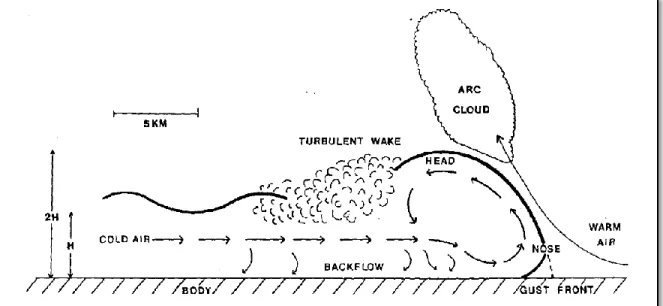
Rotors or horizontal vortices have been shown to be present at the leading edge of cold outflows in both observations (e.g., Fujita 1985; Hjelmfelt 1988; Kessinger et al. 1988; Fig. 2.5) and model simulations (e.g., Droegemeier and Wilhelmson 1987). Figure 2.6 is a schematic cross section through the gust front of a thunderstorm from Droegemeier and Wilhelmson (1987). Some of these observations and model simulations indicate that rotors may contribute to the high surface winds associated with outflow in downbursts due to stretching of vorticity when the downburst increases in size. Rotors pose a significant risk to aviation. For example, rotors from a downburst may have contributed to the 1985 crash of Delta Flight 191 at the Dallas-Fort Worth

(32)

10

(Texas) airport (Fig. 2.4; Fujita 1986). This crash led the Federal Aviation Administration (FAA) to conduct a study on how dangerous, low-level wind shear could be detected by radar and resulted in funding for the C-band Terminal Doppler Weather Radar (TDWR) program (Whiton et al. 1998).

Fig. 2.6. Schematic of a vertical cross section through a mature thunderstorm outflow. From Droegemeier and Wilhelmson (1987); based on previous work from Charba (1974), Goff (1976), Wakimoto (1982), and Koch (1984).

Vertical vortices may develop along the leading edge of the gust front as well and may have the visual appearance of a giant dust devil or dusty tornado (e.g., Fujita 1985; Wakimoto and Wilson 1989). In numerical study by Lee and Wilhelmson (1997), they found that a vertical vortex sheet develops along the leading edge of an outflow boundary when there is a component of motion in the environment (ahead of the outflow boundary) parallel to the gust front. Essentially, the interaction of air masses creates a narrow transition zone of horizontal shear aligned along the leading edge of the convergence boundary/gust front. It is assumed that horizontal shearing instability is triggered (at least primarily) by lobe and cleft instability along

(33)

11

this vortex sheet by perturbations present at the gust front. Other possible triggers may include horizontal convective roll intersections with the outflow boundary, variations in the surface roughness, or variations in the outflow thermal field. Environmental horizontal vorticity tilted upward and stretched may also play a role. These vertical vortices can grow in size have an appearance and strength of a tornado and are sometimes known as “gustnadoes” (Doswell 1985); however, there is debate whether they should be classified as tornadoes because they are a “practically ubiquitous aspect of strong convective outflows” (Markowski and Dotzek 2010) and are often not strong enough to inflict damage.

2.3 Mechanisms Driving Downbursts

Downbursts, by definition, are associated with downward (negative) vertical motion. Therefore, the vertical equation of motion can be used to determine the mechanism (i.e., dynamics) that results in the downward motion (i.e., acceleration) in downbursts. Neglecting friction, the vertical component of the equation of motion is (Houze 2014):

𝐷𝑤 𝐷𝑡 = − 1 𝜌_𝑜 𝜕𝑝∗ 𝜕𝑧 + 𝐵(𝜃𝑣∗, 𝑝∗, 𝑞𝐻) (2.1) where 𝐷𝑤

𝐷𝑡 is the total derivative of w (the vertical component of wind), z is vertical height, 𝑝 is

pressure, 𝜌 is density, 𝐵 is buoyancy, 𝜃𝑣 is the virtual potential temperature, and 𝑞𝐻 is the mixing

ratio of hydrometeors in the air (total mass of liquid water and/or ice per unit mass of air). In this form, the reference state is denoted by an “o” and the deviation from a hydrostatically balanced reference state (whose properties vary only with height) is denoted by an “*”.

The first term on the right hand side of the equation, the acceleration due to a pressure-gradient, has been shown to not contribute to the downward motion in downbursts (Kessinger et al. 1988). This is intuitive because this term would produce an upward directed pressure-gradient

(34)

12

force acting against the downdraft because of a pressure maximum at the surface (Houze 2014). In other words, it acts to decelerate the vertical velocity as it approaches the surface. Therefore, the driving mechanism for downbursts reduces to the negative contributions due to buoyancy.

Buoyancy, B, is approximated by (Houze 2014):

𝐵 ≈ 𝑔 [𝜃𝑣∗

𝜃_𝑣_𝑜+ (𝜅 − 1) 𝑝∗

𝑝_𝑜− 𝑞𝐻] (2.2) where 𝜅 = 𝑅𝑑⁄_𝑐_𝑝. 𝑅_𝑑 is the gas constant for dry air and 𝑐_𝑝 is the specific heat of dry air at

constant pressure.

Virtual potential temperature, 𝜃𝑣, is defined as the potential temperature that dry air

would have if its pressure and density were equal to those of a given sample of moist air. It can be approximated by (Houze 2014):

𝜃_𝑣 ≈ 𝜃(1 + 0.61𝑞_𝑣) (2.3) where 𝜃 is the potential temperature and qv is the is the mixing ratio of water vapor in the air.

From the equation for buoyancy (2.2), it can be seen there are three factors that affect buoyancy (Wakimoto 2001): 1) thermal buoyancy, 𝜃𝑣∗

𝜃_𝑣𝑜; 2) perturbation pressure buoyancy,

(𝜅 − 1)𝑝_𝑝∗

𝑜, and 3) condensate (precipitation) loading, 𝑞𝐻.

For the first term, the negative contribution to the thermal buoyancy term can be increased by phase changes and the associated absorption of latent heat (i.e., melting and/or evaporating) from hydrometeors (i.e., 𝜃_𝑣∗ becomes more negative). Note that there will be a competing force of adiabatic warming with any downward motion. The temperature deficit for 𝜃𝑣∗ due to evaporation can be calculated by the following relationship (Wakimoto 2001):

𝜃𝑣∗ = −𝐿

𝑞_𝑟

(35)

13

where L is the latent heat of vaporization and qr is the mixing ratio of rain water that has

evaporated. A similar formulation may be used to calculate the temperature deficit for 𝜃_𝑣∗ due to melting using the latent heat of fusion.

The second term indicates that an air parcel will accelerate upward if it is at a lower pressure than its surroundings (Wakimoto 2001). It has been primarily shown to counteract strong negative thermal buoyancy for overshooting tops (Schlesinger 1980). Otherwise, not much emphasis has been placed in studying its effects (Wakimoto 2001) and the assumption is it does not play a significant role in downbursts.

The third term indicates that the downward drag of precipitation will result in negative buoyancy through the force of gravity acting on the hydrometeors (i.e., precipitation loading). Therefore, it can be surmised that the primary driving mechanisms for the downward motion in downbursts (as deduced through the buoyancy term of the vertical equation of motion) are 1) thermal buoyancy through evaporation and/or melting of hydrometeors and 2) precipitation loading.

If the vertical motion in a downburst can be deduced from the vertical equation of motion (or through some other method such as dual-Doppler analysis), other dynamical quantities can be approximated. The maximum stagnation pressure perturbation, 𝑝𝑚𝑎𝑥∗ , at the center of the

downburst can be approximated by the following relationship based on Bernoulli’s equation (Stull 2017): 𝑝_𝑚𝑎𝑥∗ ₌ 1 𝜌_𝑜[ 𝑤_𝑑2 2 − 𝑔𝜃𝑣∗𝑧 𝜃_𝑣_𝑜 ] (2.5) where wd is the likely peak downburst speed at height z well above the ground.

There are two contributions to the increased pressure at the surface in a downburst. The first term is due to dynamics (i.e., pressure increase due to motion) and the second term due to

(36)

14

thermodynamics (i.e., pressure increase due to the added weight of cold air). Note that this equation assumes a steady-state process.

Using 𝑝_𝑚𝑎𝑥∗ , the change of outflow wind magnitude can be approximated using the horizontal pressure gradient force (Stull 2017):

𝜕𝑀 𝜕𝑡 = 1 𝜌_𝑜 𝑝_𝑚𝑎𝑥∗ 𝑟 (2.6) where M is the outflow wind magnitude and r is the radius of the downburst (assuming it roughly equals the radius of the mesohigh). In practice, this is usually an approximate (order of magnitude) value since the pressure gradient will vary in both space and time.

Assuming r is constant, the maximum wind speed at the surface (i.e., outflow winds) will increase as 𝑝_𝑚𝑎𝑥∗ increases. If r increases, 𝑝_𝑚𝑎𝑥∗ would have to increase further to compensate for the increase in r. Therefore, the maximum wind speed at the surface is controlled by 𝑝𝑚𝑎𝑥∗ and

the r. 𝑝_𝑚𝑎𝑥∗ is controlled by peak downburst speed and the temperature deficit in the mesohigh. The previous assessment of the vertical equation of motion (2.1) and buoyancy (2.2) fit our current understanding on the initiation of downbursts from observation-based studies (e.g., Atlas et al. 2004; Wakimoto and Bringi 1988; Wakimoto et al. 1994) and from idealized numerical simulations (e.g., Proctor 1988, 1989; Srivastava 1985, 1987).

From these studies, it is understood that precipitation microphysical processes in a suitable ambient thermodynamic environment are important in producing downbursts. For dry downbursts, the sublimation of snowflake particles through a deep, dry adiabatic layer has shown to be effective in producing downbursts (Proctor 1989; Wakimoto et al. 1994). For wet downbursts, the ambient thermodynamic environment tends to be more humid and stable. In these situations, precipitation loading becomes more important for driving the initial downdraft

(37)

15

at mid-levels. As the environmental lapse rate decreases (increases), higher (lower) water content is needed for a downburst (Fig. 2.7; Srivastava 1985).

Fig. 2.7. Results of a one-dimensional time dependent nonhydrostatic cloud model of a downdraft. Plotted numbers are vertical air velocity (m s-1) at a level 3.7 km below the top of the downdraft (~850 hPa) as a function of the lapse rate in the environment and total liquid water mixing ratio at the top of the downdraft. Numbers on top scale indicate the radar reflectivity and rain rate at the top of the downdraft. Curved dotted line separates downbursts (<20 m s-1) from less intense downdrafts. It was found that as the environmental lapse rate decreases (increases), higher (lower) water content is needed for a downburst. From Srivastava (1985).

Observations and simulations also suggest that melting hailstones are important for wet downbursts (e.g., Atlas et al. 2004; Fu and Guo 2007; Proctor 1989; Srivastava 1987; Wakimoto and Bringi 1988). Fu and Guo (2007) simulated a downburst using a three-dimensional cloud

(38)

16

model that included hail-bin microphysics. They found that the downburst primarily was produced by hail-loading and was enhanced by cooling processes that were due to melting hailstones and the evaporation of raindrops. Proctor (1989) hypothesized that hail-loading is especially important in more stable environments because the cooling effect is delayed to lower elevations.

It has also been found that dry downbursts tend to have a small negative temperature perturbation (i.e., cooling) over a deep column. In contrast, wet downbursts tend to have a relatively larger, negative temperature perturbation over a shallower column near the surface (Proctor 1989). Proctor (1989) also found warming aloft with wet downbursts, indicating that precipitation loading is necessary to overcome positive temperature buoyancy.

It can be surmised from these studies that precipitation loading (including hail) is much more important for wet downbursts than dry downbursts. Though not explicitly stated yet, one can assume that if a wet downburst occurs in an environment that is favorable for dry downbursts (i.e. steep, low-level lapse rates), both phase changes and precipitation loading may have significant contributions to negative buoyancy.

2.4 Radar Observations of Downbursts

The characteristic radar signature associated with downbursts is a low-level radial divergence signature. Wilson et al. (1984) defined the diverging signature for a microburst having a velocity differential ≥ 10 m s-1 at an initial distance ≤ 4 km.

(39)

17

Fig. 2.8. Horizontal radar reflectivity factor (ZH) and radial velocity (VR) from KOUN on 15 June 2011 at 0022 UTC. The characteristic low-level radial divergence signature associated with the downburst is seen. Plotted using GR2Analyst.

While the low-level divergence signature is useful in the detection of an ongoing downburst, it does not provide any lead time. Prior to dual-pol radars, descending reflectivity cores (DRCs) were found to occur prior to downbursts (e.g., Roberts and Wilson 1989); however, it is difficult to deduce dominant hydrometeor types and microphysical properties with single-pol radars. There have been some studies that have utilized dual-pol radar observations for downbursts (e.g., Atlas et al. 2004; Kuster et al. 2016; Richter et al. 2014; Scharfenberg 2003; Suzuki et al. 2010; Tuttle et al. 1989; Wakimoto and Bringi 1988), which generally have found that melting hail and associated mixed-phase hydrometeors are an important aspect for downbursts due to cooling from melting and precipitation loading. This matches the findings from the simulations that were discussed previously in this chapter.

Wakimoto and Bringi (1988) found near-zero ZDR surrounded by positive ZDR in the main precipitation core within a microburst-producing downdraft, which they determined was associated with a strong downdraft composed of melting hail (Fig. 2.9). Scharfenberg (2003) and Suzuki et al. (2010) both noted reduced ρhv in the descending core. The ρhv reduction was

(40)

18

attributed to mixed-phase hydrometeors (i.e., mixture of rain and hail) in the downburst. From these studies, it is clear the advantage of dual-pol radars when studying downbursts is a better understanding of hydrometeor evolution and associated microphysical properties.

Fig. 2.9. Vertical cross section showing dual-polarization Doppler radar measurements obtained in a thunderstorm in northern Alabama during the MIST project. Note the presence of a ZDR hole within the main precipitation core within a microburst-producing downdraft, which indicates the presence of melting hail. Reflectivity data are presented in contours of dBZ. ZDR are shown in dB units. Arrow indicates location of the center of a surface microburst. From Wakimoto and Bringi (1988).

(41)

19

2.5 Summary

Overall, a downburst occurs when an intense downdraft reaches the surface and the attendant cold pool spreads out as a density current. The primary driving mechanisms for the downward motion in downbursts are 1) thermal buoyancy through evaporation and/or melting of hydrometeors and 2) precipitation loading. Unsurprisingly, precipitation loading (including melting hail) is much more important for wet downbursts than dry downbursts. PRD have been utilized in some downbursts studies, which have shown the importance of melting hail in downbursts.

The maximum wind speed at the surface is controlled by horizontal pressure gradient force at the surface (i.e., the maximum pressure perturbation and radius of the downburst). As shown by Bernoulli’s equation, the maximum pressure perturbation at the surface is determined by peak downburst speed and the temperature deficit in the mesohigh. The peak downburst speed is controlled by the previously mentioned driving mechanisms for downward motion.

The aforementioned summary on downbursts serves as motivation for this study. It is evident that the hydrometeor evolution and associated microphysical processes within the parent thunderstorm is important in the dynamics of downbursts. By using PRD, a better understanding of the microphysical evolution of precipitation is possible.

(42)

20

Chapter 3 : Observation Tools

The primary observation tools used in this study include S-band radars, a mobile X-band radar, and a 1-min surface observation station. Details on the radars and the surface station are provided in this chapter.

3.1 KOUN WSR-88D

The KOUN S-band (~11.09 cm) WSR-88D radar, located in Norman, Oklahoma, collected polarimetric radar observations of the downburst and its parent thunderstorm. The National Weather Service (NWS) installed the prototype dual-pol upgrade for the WSR-88D radars on the KOUN radar (Saxion and Ice 2012). It is maintained by the National Severe Storms Laboratory (NSSL).

KOUN was scanning with Volume Coverage Pattern (VCP) 11, which was a VCP frequently used for severe thunderstorms in the past (Office of the Federal Coordinator for Meteorological Services and Supporting Research 2016). In this scanning strategy, each volume scan takes approximately five minutes and includes 360° plan position indicator (PPI) scans (i.e., conical scans) collected at 14 different elevations. The PPI scans are taken at approximately 0.5°, 1.5°, 2.4°, 3.4°, 4.3°, 5.3°, 6.2°, 7.5°, 8.7°, 10.0°, 12.0°, 14.0°, 16.7°, and 19.5° elevation angles.

The radial sampling resolution was 250 m and azimuth increment was 0.5° for the lowest two elevation scans (0.5° and 1.5°). The two lowest elevation angles are split cut elevations, where there is a low PRF contiguous surveillance (CS) and high PRF contiguous Doppler (CD) scan. Reflectivity and PRD are processed from the CS scan. At higher elevations, the azimuth increment is 1.0°. Radar data were manually dealiased using the National Center for Atmospheric Research (NCAR) Earth Observing Laboratory’s (EOL) solo3 software package.

(43)

21

The KOUN radar was within 5 km of the downburst, providing excellent resolution and low-level coverage for this event. However, because the highest elevation PPI was at 19.5°, a limitation is the storm top was not sampled due to the radar cone of silence. As the storm approached the radar, less of the storm was sampled aloft. KOUN WSR-88D radar data were obtained from the National Climatic Data Center (NCDC 2011a).

3.2 KTLX WSR-88D

The KTLX S-band WSR-88D radar, located in Norman, Oklahoma, also collected radar observations of the downburst and its parent thunderstorm. In 2011, KTLX had not yet been upgraded to dual-pol; otherwise, its radar characteristics are similar to KOUN. KTLX was located ~20 km to the northeast of KOUN and provided limited dual-Doppler coverage. Dual-Doppler coverage was limited because the between-beam angle was small for much of the thunderstorm’s life cycle. KTLX WSR-88D radar data were obtained from the NCDC (NCDC 2011a).

3.3 RaXPol

RaXPol (Fig. 1; Pazmany et al. 2013) collected high spatiotemporal resolution of the downburst and its associated gust front and rotor within close range. Data were collected by Jeff Snyder and Andrew Pazmany. RaXPol has a 2.4-m-diameter dual-pol parabolic dish antenna on a high-speed pedestal. The 20-kW transmitter can generate pulse compression and frequency-hopping waveforms. Frequency frequency-hopping allows for more independent samples when compared to no frequency hopping, which allows RaXPol to scan much more rapidly than conventional radars. Pazmany et al. (2013) contains more technical details on RaXPol and its radar system.

(44)

22

For this event, one 360° PPI elevation scan took ~6-7 sec with elevation scans every 2° from 1.0° to 27.0°. An entire volume scan took ~1 min and 40 sec. Note for this event and others collected in 2011 (Houser et al. 2015; Pazmany et al. 2013) the RaXPol data on the lowest elevation scan were actually data collected during the downward spiral from the previous higher elevation scan (this was the first year RaXPol was used). Therefore, the 1.0° elevation scan is not useful for analysis or reconstructed RHIs (i.e., the lowest scan with no data quality issues is 3.0°).

The radial sampling resolution was 75 m and azimuth increment was ~1.1°. The Nyquist velocity was 30.8 m s-1. As with the WSR-88D data, radar data were manually dealiased using the NCAR EOL’s solo3 software package. Data where the SNR were less than 5 dB were removed.

As with the WSR-88D, the downburst and its intense winds were moving toward and directly impacted the radar. The RaXPol data collection began later in the thunderstorm’s life cycle when compared to the WSR-88D data. Therefore, less of the storm was sampled aloft when compared to the WSR-88D data.

(45)

23

Fig. 3.1. Photo of RaXPol collecting data from the downburst in Norman, Oklahoma, on 14 June 2011. Note that the wet downburst is seen in the background. Photo courtesy Robin Tanamachi.

3.4 Mesonet

Surface observations were provided by the Oklahoma Mesonet, which is maintained by the Oklahoma Climatological Survey (Oklahoma Climate Survey 2011). The Oklahoma Mesonet (Brock et al. 1995; McPherson et al. 2007) is a network of over 100 automated weather stations covering Oklahoma. There is a Mesonet station in Norman, Oklahoma, nearly collocated with the KOUN radar. The Mesonet station recorded 1-min data from the downburst. The data collected include temperature and relative humidity at 2 m, wind speed and direction at 10 m, station atmospheric pressure, and tipping-bucket precipitation. One tip is equivalent to 0.254 mm

(46)

24

of rainfall. The 10-m maximum wind speed (i.e., wind gust) is the highest 3 s sample within the 1-min interval. The unique 1-min temporal resolution provides highly detailed information about the surface conditions beneath the downburst.

3.5 Observation Locations

During the data collection, KOUN was located approximately 256 m to the southeast of RaXPol. The Norman Mesonet station was located approximately 221 m to the southwest of RaXPol. For practical purposes, these are considered nearly collocated. Figure 3.2 is a map with the locations of these three observation sources. Note that KTLX is not shown on this map.

Fig. 3.2. Map of RaXPol, KOUN, and the Norman, Oklahoma, Mesonet locations during data collection. KOUN was located approximately 256 m to the southeast of RaXPol. The Norman Mesonet station was located approximately 221 m to the southwest of RaXPol. Plotted using Google Earth.

(47)

25

Chapter 4 : Downburst Overview, Environment, and Surface Observations

3

An event overview of the 14 June 2011 Norman, Oklahoma, downburst is provided in this chapter. This includes an overview of damage reports, the mesoscale and thermodynamic environment, and 1-min Oklahoma Mesonet surface observations.

4.1 Event Overview

The downburst affected Norman, Oklahoma, in the early evening between 7:29 to 7:50 pm CDT (0029 to 0050 UTC) on 14 June 2011 (15 June 2011 UTC). Surface winds in excess of 35 m s-1 (>80 mph) and hailstones in excess of 4 cm diameter were reported from the storm in Norman, Oklahoma (Fig. 4.1; NOAA/NCDC 2011). The maximum wind gust measured was 36.7 m s-1 in southeast Norman, and the largest hailstone reported was 4.4 cm. The maximum wind gust may have been underestimated because the anemometer recorded the 36.7 m s-1 before malfunctioning due to windblown hail. As a result of the downburst, widespread wind damage occurred across Norman (Fig. 4.2a), including at Max Westheimer Airport (Fig 4.2b,c). Numerous power lines were snapped and over 33,000 residents of Norman lost power; some residents lost power for over 24 hours. Nearly horizontal, windblown hailstones damaged automobiles, house siding, and store signs. Figure 4.1 is a summary of the official NWS storm reports and episode narrative associated with the downburst. The area of damage from the downburst was over 4 km in length; therefore, the downburst can be classified a macroburst by size.

3_{Adapted from: Mahale, V. N., G. Zhang, and M. Xue, 2016: Characterization of the 14 June 2011 Norman,}

Oklahoma, downburst through dual-polarization radar observations and hydrometeor classification. J. Appl. Meteor. Clim., 55, 2635–2655.

(48)

26

Fig. 4.1. Official storm reports and event narrative for the Norman, Oklahoma, downburst from the National Centers for Environmental Information (NCEI) Storm Events Database. The table abbreviations are: St. is state; T.Z. is time zone; Mag is magnitude; Dth is deaths; Inj is injuries; PrD is property damage estimate; and CrD is crop damage estimate. From NOAA/NCDC (2011).

(49)

27

Fig. 4.2. Map of wind damage reports (courtesy National Weather Service Norman, Oklahoma), (b) photo of the downburst from north Norman, and (c) photo of damage at Max Westheimer Airport. Photos courtesy Robin Tanamachi.

4.2 Mesoscale and Thermodynamic Environment

The thermodynamics of the atmosphere were highly conducive for storms to produce severe downbursts in Central Oklahoma on 14 June. The Norman (KOUN) sounding at 0000 UTC on 15 June 2011 was the closest spatiotemporal sounding to the downburst (Fig. 4.3). The downburst affected Norman just after 0020 UTC; therefore, the sounding should be a reasonable representation of the pre-storm environment.

(50)

28

As shown by the calculated parameters, the atmosphere was favorable for organized severe thunderstorms with both moderate instability and vertical wind shear. A nearly dry adiabatic (well-mixed) layer existed below the cloud layer, which is favorable for downbursts (Srivastava 1987) and results in large downdraft convective available potential energy (DCAPE). DCAPE is defined as the maximum increase in kinetic energy (per unit mass) that could result from evaporative cooling from some height to the surface (Emanuel 1994). Note that this sounding is not a classic wet downburst sounding (i.e., Atkins and Wakimoto 1991) due to the relatively dry boundary layer and steep low-level lapse rates.

A couple parameters that specifically have been computed to assess downburst potential are the Δθe between the near-ground maximum and the mid-level minimum (Atkins and Wakimoto 1991) and the Wind INDEX or WINDEX (McCann 1994). The WINDEX formula is:

𝑊𝐼 = 5[𝐻_𝑚𝑅_𝑄(Γ2_{− 30 + 𝑄}

𝐿− 2𝑄𝑚)] 0.5

(4.1) where Hm is the height of the melting level in km above ground, RQ = QL/12 but not greater than 1, Γ is the lapse rate in °C per km from the surface to the melting level, QL is the mixing ratio in the lowest 1 km above the surface, and Qm is the mixing ratio at the melting level. The formula is an empirical relationship.

The Δθe of 18.4 K is lower than the 20 K threshold for wet downbursts found in Atkins and Wakimoto (1991); however, this could be attributed to not being a classic wet downburst sounding. Finally, the WINDEX was calculated to be 30.4 m s-1 (59 knots), which underestimated the > 35 m s-1 measured surface winds.

(51)

29

Fig. 4.3. Upper-air sounding and hodograph from Norman, Oklahoma (KOUN) at 0000 UTC 15 June 2011. Temperature is denoted by the red line and dew point by the green line. The purple line is the virtual temperature correction, and the turquoise line represents the parcel path for surface-based parcel. Plotted using The Universal Rawinsonde Observation (RAOB) program.

On the mesoscale, a cold front was located across central Oklahoma (Fig. 4.4). The temperature change across the cold front was weak (~3 to 4°C). The wind shift along the cold front was nearly 180°; thus, surface convergence was present along the boundary. The convergence along the cold front was also detected by the KTLX WSR-88D radar in the velocity data (not shown). This was coincident with a weak line of ZH, which indicates there was a buildup of particulates and insects along the convergence line. KTLX was not dual-pol capable