Accepted on 7/21/2011 in: ASCE Journal of Waterway, Port, Coastal, and Ocean Engineering
STATIC ANALYSIS OF THE LUMPED MASS CABLE
MODEL USING A SHOOTING ALGORITHM
Marco D. Masciola1, Meyer Nahon1, and Frederick R. Driscoll 2 ABSTRACT
This paper focuses on a method to solve the static configuration for a lumped mass cable system. The method demonstrated here is intended to be used prior to performing a dynamics simulation of the cable system. Conventional static analysis approaches resort to dynamics relaxation methods or root–finding algorithms (such as the Newton–Raphson method) to find the equilibrium profile. The alternative method demonstrated here is general enough for most cable configurations (slack or taut) and ranges of cable elasticity. The forces considered acting on the cable are due to elasticity, weight, buoyancy and hydrodynamics. For the three–dimensional problem, the initial cable profile is obtained from a set of two equations, regardless of the cable discretiza-tion resoludiscretiza-tion. Our analysis discusses regions and circumstances when failures in the method are encountered.
INTRODUCTION
Modeling and simulation of cable systems is a current and ongoing research in-terest among members of the oceanographic community. The practices employed to represent such systems vary, and the model used to perform the simulation depends on specific needs of the end user. Perhaps the simplest cable representa-tion is demonstrated in Malaeb (1982), where the effects of cable flexibility, but not mass, are considered by treating the cable as a linear spring. Others have used continuous systems to model the effects of tether weight to obtain the static cable forces (De Zoysa 1978; Friswell 1995). Generally, as the scale of the system
1Department of Mechanical Engineering, McGill University, Montreal, Quebec, H3A 2K6,
Canada
2National Renewable Energy Laboratory, Marine and Hydrokinetic Technologies, Golden,
and length of the cable increases, the cable dynamics (such as propagating inter-nal waves) become increasingly important (Mekha et al. 1996). In response, a discretized cable model, such as one using a finite element representation, should be used when these effects are anticipated to be important.
The discretized cable system presented in this paper is modeled using a lumped mass approach. This technique was developed heuristically as an ex-tension of the finite element process and is based on a reorganization of the mass matrix (Walton and Polacheck 1960; Merchant and Kelf 1973). This simplifica-tion allows the dynamics problem to be computed more efficiently compared to strict finite element derivations, but without a significant compromise to accu-racy (Ketchman and Lou 1975; Kamman and Huston 1999). The model described here was developed in Driscoll (1999), though similar lumped mass representa-tions have appeared elsewhere (Huang 1994; Kamman and Huston 1999; Nahon 1999; Chai et al. 2002; Williams and Trivaila 2007). Before beginning a simu-lation, the equilibrium configuration must first be determined. This ensures the ensuing motion is due to outside sources and not from a force imbalance in the initial conditions. A primary challenge associated with discretized cable modeling is generation of the initial equilibrium profile, and this trouble is encountered be-cause cables lack the ability to support compressive loads (Webster 1980; Shugar 1991; Wu 1995; Gobat 2002).
To begin this exploration of the static cable problem, a description of the lumped mass dynamics model is presented. Conventional solution techniques are then described and deficiencies in the most commonly used methods are high-lighted. A new solution approach to this problem is then discussed, which relies on a shooting algorithm to converge onto the static cable configuration. A good background resource documenting the shooting method and its application to cables is given in De Zoysa (1978); however, De Zoysa’s implementation is con-cerned with continuous cable models, which does not give the solution to the lumped mass system. Our implementation extends De Zoysa’s approach to the lumped mass cable model. This discussion concludes by analyzing regions where the shooting method does not converge, and reasons why these failures occur. Failures are more likely to be encountered in systems represented with straight rigid elements, as opposed to those systems that consider bending stiffness (Web-ster 1980). The straight–element lumped mass representation is analyzed here since 1) it is more sensitive to initial conditions compared to other models, and 2) the lumped mass representation is a commonly used modeling theory.
LUMPED MASS CABLE MODEL
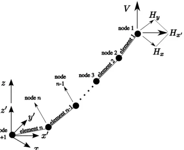
A detailed account of the lumped mass cable model is contained in Nahon (1999), but for the purpose of clarity and completeness, a brief description is provided here. The cable is discretized into n elements and n + 1 nodes and is suspended between two endpoints, Fig. 1. An inertial reference frame{x , y , z} is defined with the origin at the bottom node and with thez–axis vertical positive upward. Mass is concentrated at the nodes, and the nodes are connected by visco–
elastic elements. Each element has an unstretched length equal to Lu = L0/n and a stretched length of li, where L0 is the total unstretched length of the cable. At the uppermost node, i= 1, external forces Hx, Hy and V are applied,
corresponding to the horizontalx, horizontal y and vertical z force components. Vector ri defines the position of each node in relation to node n+ 1. For this
implementation, the position of the first node is centered at r1 = {lx , ly , h}T,
and the final node at rn+1 = {0, 0, 0}T. The cable is assumed to be uniform, thusA and E, the cross sectional area and modulus of elasticity, are constant.
The equation of motion for each node can be constructed as follows (Nahon 1999): M¨ri = (Ti−1+Pi−1)−(Ti+Pi) + 1 2(Di−1+Di) + 1 2g( ˜mi−1+ ˜mi) (1) whereTi is the elastic tension in theith cable element,Pi is the internal damping
force,Di is the drag force on theith element, ˜mi is the net mass (after accounting
for buoyancy) of the node in the fluid it is immersed in, and g ={0, 0, −g}T is the gravitational constant vector. SinceLu is assumed to be the same for each
element, we set ˜mi = ˜m. Mis a diagonal matrix containing the mass of the node.
When solving the statics equations, the internal damping term is set to zero since the nodes are not moving relative to each other. The drag force, however, remains since the surrounding fluid (air or water) may itself be moving. We assume that each element behaves as a linear spring, and the tension generated is:
Tiq = AE
Lu
(li−Lu) (2)
where li is the stretched cable length and equal to li = kri+1−rik. The result
for Tiq in Eq. 2 is the force magnitude tangential to the element, and must be transformed into components in the reference frame in which Eq. 1 is written in (usually the inertial frame). Equation 1, in component form, becomes:
m{¨ri}x = Tiq−1sinθi−1cosφi−1 −(Tiqsinθicosφi) + 1 2({Di−1}x+{Di}x) (3a) m{¨ri}y =− Tiq−1sinφi−1 + (Tiqsinφi) + 1 2 {Di−1}y+{Di}y (3b) m{¨ri}z = T q i−1cosθi−1cosφi−1 −(Tiqcosθicosφi) + 1 2({Di−1}z+{Di}z) (3c) where the Euler angles are determined from:
θi = atan2 ({ri−ri+1}x , {ri−ri+1}z) (4a) and: φi = atan2 − {ri−ri+1}y , rji −ri x/sinθi if cosθi <sinθi (4b) φj = atan2− rj−rj+1 ,
FIG. 1. A lumped mass cable model arranged in the xyz frame. In the absence of aero / hydrodynamics forces, the cable lies in the vertical x′z′
reference frame.
A variety of models are available to obtain the drag vectorDi, but in this
imple-mentation, the method discussed in Nahon (1999) is used.
CONVENTIONAL STATIC ANALYSIS TECHNIQUES
Webster (1980) and Wu (1995) provide a comprehensive review of static anal-ysis of flexible structures such as cables, inflatable shells and elastic membranes. Webster solves the problem using a variety of techniques and demonstrates the success of each method varies greatly depending on the nature of the problem. Wu narrows the analysis to cables and improves the methods studied in Webster con-siderably. An approach known as dynamic relaxation is perhaps the least difficult to implement since it uses the existing dynamics model to process the solution. Dynamic relaxation is a procedure that finds the static solution by performing a simulation with the system not in static equilibrium. The equations of motion are integrated (i.e. the system is simulated) until transient motions dissipate. While convergence is virtually guaranteed with the dynamic relaxation approach, it is not very efficient, particularly if only small (order 10−6) accelerations for¨r
i are
tolerated.
Another widely used approach implements a Newton–Raphson solver (or com-parable) root finding algorithm to find equilibrium positions for the nodes. In this document, we refer to this procedure as theincremental method. This approach operates by seeking values of ri that result in zero acceleration at each node, i.e.
the left hand side of Eq. 1. Under certain conditions, however, the solver may not converge to a solution. The source for non–convergence is attributable to either a poor initial guess or an ill–conditioned Jacobian matrix. Generally, the lower the stiffness of the system, the more likely convergence will occur. In the case of a
stiff system, the initial guess must be more precise, and reasonably estimating a good initial guess becomes more difficult. One way of circumventing this obstacle is as follows:
1. We want to solve the statics problem for a cable with an elasticity of Ef.
This is achieved by first relaxing the material modulus to E0, where E0 is low enough that the Jacobian is no longer ill–conditioned.
2. Set up the initial guess x0, which is defined as a vector containing the initial estimate for each node position.
3. Solve the statics problem with E0 using the root–finding algorithm. We now obtain a solution y0 describing the nodes positions at E0.
4. Increase E0 by ∆E, i.e., E1 =E0+ ∆E.
5. For the next iteration, set the initial guess to the final solution from the previous iteration, x1 =y0.
6. Repeat the steps 3 – 5 until Ei =Ef.
Although the incremental method was shown by Webster to have the highest probability of failing, we investigate this solution method in greater detail since this technique is commonly used in the cable modeling community. An alterna-tive remedy to the incremental method is proposed in Peyrot (1980), where an artificial stiffness term is included to improve convergence characteristics.
Zueck (1995) demonstrates the use of a highly robust solver that relies on the approach presented in Powell and Simons (1981). This robust tool, which is described as the “event–to–event solution strategy”, is demonstrated by solving the challenging problem posed in Webster (1980). While Webster could achieve a solution through his viscous relaxation technique in 28 iterations, only two iterations are needed with Zueck’s method. This identical robustness test will also be performed on the shooting method developed in this paper.
Incremental Method Limitations
The statics equation for a cable arrangement is obtained by setting the left hand side of Eqs. 3a–3c to zero. This analysis presumes the two cable end point positions, r1 and rn+1, are known, and nodes 2 through n are unknown. The unknown node displacements are obtained by simultaneously solving Eqss 3a–3c for the intermediate nodes, which implies 3×(n−1) non–linear algebraic equations are simultaneously solved. This solution method utilizes a root finding algorithm, specifically the Newton–Raphson method, to find the zeros of Eqs. 3a–3c. It is well known the solution for a catenary is unique, and only one real solution exists (Vesli´c 1995).
The proximity of the initial guess to the solution greatly impacts the success of convergence. Generally, if the element stiffness is low, the Newton–Raphson method forgives a poor initial guess, thus allowing convergence. As stiffness increases, more accurate initial guesses must be used. One way of measuring how
loose the initial guess can be is through the condition numberc (Strang 1981):
c=kJk
J−1
(5)
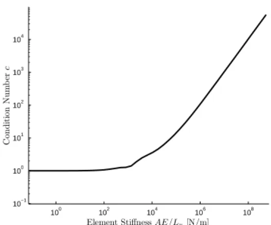
whereJ is the Jacobian at convergence. The smallest valueccan attain isc= 1. A high value for c implies that J is ill–conditioned, and as a consequence, the Newton–Raphson algorithm may not converge onto a solution when a poor initial estimate is used. In Fig. 2, the relationship between condition number and cable element stiffness is given. A stiffness of AE/Lu ≈100 N/m marks the threshold
at which the condition number begins an upward trend. As the stiffness increases, the initial guess must be closer to the actual solution to ensure convergence. Note that Lu = L0/n, and as the discretization becomes finer, the condition number will increase. In summary, the incremental method, in conjunction to using a Newton–Raphson root finding algorithm, can converge onto a solution provided that 1) the condition number is low and / or 2) the initial guess is near the solution for Eqs. 3a–3c.
100 102 104 106 108 10−1 100 101 102 103 104
Element StiffnessAE/Lu[N/m]
C on d it ion Nu m b er c
FIG. 2. Condition number as a function of the element stiffness. As the
ele-ment stiffness k=AE/Lu =nAE/L0 becomes larger, the condition number
increases.
PROPOSED SHOOTING METHOD
The shooting method is a mathematical procedure applied to boundary value problems with unknown initial states. For the case of a cable stretched between two points, the solution is obtained by iterating unknown cable properties un-til the desired boundary conditions (the cable end points) are achieved. Several researchers have demonstrated the application of the shooting method to under-water continuous cables (De Zoysa 1978; Friswell 1995). More recently, Gobat (2002) has utilized the shooting method to obtain a statics solution for his finite difference cable model, though the model Gobat demonstrated is fundamentally different from the lumped mass cable.
To simplify analysis, drag forces are temporarily neglected. The configuration for the system without drag will serve as a guess of the cable profile with drag in affect. In the absence of drag forces, the cable lies in a vertical plane defined as the xz plane. This reduces Eqs. 3a–3c to two equations, namely {¨ri}x′ and
{¨ri}z′, Fig. 1. The z′–axis is aligned with the gravitational vector and in the
same direction as the inertial frame z–axis. The x′–axis is perpendicular to z′ and points from the origin to the point {lx , ly , 0}, i.e. the projection of r1 onto the inertial xy plane. Angle α distinguishes the x and x′ axes. The cable node positions in xyz are obtained from {ri}xyz =Rα{ri}x′y′z′, where Rα is the
rotation matrix fromx′y′z′ coordinates into xyz.
The position of the starting node is r1 = {lx , lh , 0}T, and the desired
po-sition of the terminating node is rf = {0, 0, 0}T. The horizontal (Hx′) and
vertical (V) forces applied at the uppermost cable node are estimated. A force– balance equation is then constructed at the first node, and the unknowns at that node are obtained algebraically. In our case, the unknowns are the inclination angle θi and the stretched element length li. Once θi and li are known, the
po-sition of the subsequent node, ri+1, can be determined. This process is repeated for successive nodes until the final nodern+1 is reached. The goal is to minimize the error krf −rn+1k such that the final node position matches the desired end
node location. This process then refines the applied forces Hx′ and V using a
root finding algorithm until the error is acceptably small. These steps are now discussed in more detail.
Initial Estimates for Hx′ and V
The initial estimates for Hx′ and V are found by simultaneously solving the
following elastic catenary equations for a continuous cable (Irvine 1992):
h= Hx′L0 W s 1 + V Hx′ 2 − s 1 + V −W Hx′ 2 +W L0 AE V W − 1 2 (6a) lx′ = Hx′L0 W sinh−1 V Hx′ sinh−1 V −W Hx′ + W AE (6b) whereW is the weight of the entire cable. The initial guess forV is equal to the cable weightW, and Hx′ is set to unity.
Node Projection
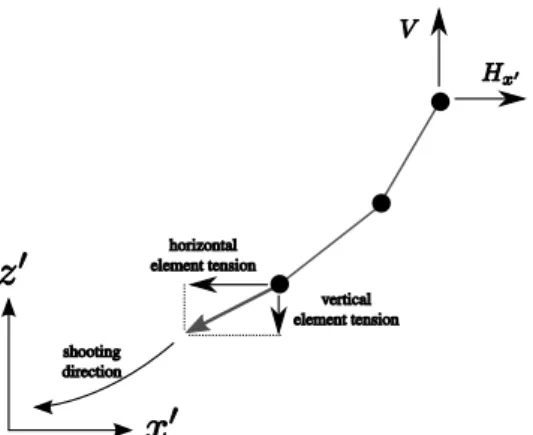
For the cable to remain in equilibrium, the tension in a given element must balance the applied external forces, Fig. 3. This process starts at node 1 since the applied forces,Hx′ andV, are known. The following observations are made: 1) in
the absence of hydrodynamic forces, the horizontal force is constant throughout the cable and equal toHx′ if the system is to remain in equilibrium; 2) the vertical
gm˜. Thus, the vertical force component at element i is: Tiqcosθi =V −g 1 2m˜ + i−1 X k=1 ˜ m ! (7) To be consistent with Eq. 1, a 1/2 ˜m term is included in Eq. 7 because half of the adjacent element’s mass is lumped into the first node. Since mass is concentrated at the node (and not along the element), each element constitutes a two force member. Sufficient information is now available to solve for the angle of inclination,θi, of the element:
θi = atan2 ( Hx′ , V − 1 2gm˜ + i−1 X k=1 gm˜ !) (8) Combining Eq. 2 and Eq. 7, the stretched element length is:
li = Lu V −1 2gm˜ + Pi−1 k=1gm˜ AEcosθi +Lu (9)
Beginning with node i = 1 as the starting point, subsequent position vectors along the cable array can be obtained from:
ri+1 =ri−liuˆi (10)
where ˆui = {sinθi , 0, cosθi}T. Once the recursion ends, a set of vectors (ri)
describing the position of each node are obtained; however, we have not yet arrived at the final solution since the last node in Eq. 10,rn+1, does not match the desired position, rf. The error krf −rn+1k is minimized by including equations
Eqs. 7–10 in a Newton–Raphson routine, where the applied forcesHx′ andV are
iterated variables. The process ends when:
krf −rn+1k ≤ǫ (11)
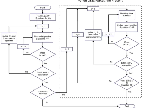
In Fig. 8, the left hand portion of the flow chart details the process outlined in this section.
Solution with Aero / Hydrodynamic Drag
The drag forces, being dependent on how the cable is oriented in the fluid flow field, are first estimated using a reference pose of the cable system. We do this by first finding the cable shape without the drag forces then apply a transformation on Eq. 10 to obtain the reference positions in thexyz frame. The node positions, element angles and lengths calculated without the drag forces are denoted asr0
i, θ0
i,l0i, respectively. Then, the drag vector D0i is evaluated based onr0i. The angle θji in the presence of hydrodynamic forces can then be calculated from:
with: Fx =Hx+ 1 2 Dj−1 i x+ i−1 X k=1 Dj−1 k x (13a) Fz =V + 1 2 Dj−1 i z−gm˜ + i−1 X k=1 Dj−1 k z−gm˜ (13b) The superscript indexj refers to the outer loop drag force iterations. If cosθij ≥ sinθij, the angle φji is:
φji = atan2 −Fy , Fx sinθij (14) Otherwise, if cosθij <sinθji
φji = atan2 −Fy , Fz cosθij (15) where Fy =Hy + 1 2 Dj−1 i y+ i−1 X k=1 Dj−1 k y (16)
The stretched length of the element is:
lij = LuFz
AEcosθji cosφji +Lu (17)
Subsequent node positions can then be obtained from Eq. 10, this time with:
ˆ
ui =
sinθijcosφji , −sinφji , cosθji cosφji T
The initial estimates for Hx and Hy are based on a projection of Hx′ on the xy
plane. As in the preceding section, a Newton–Raphson procedure is then used to find values ofHx,Hy andV that minimizekrf −rn+1k. Each time new values for Hx,Hy andV are estimated, the drag forcesDji are recalculated for the updated
cable profile, and this procedure repeats until the following criterion, along with Eq. 11, are met:
k∆Dk= Dj−1−Dj ≤δ (18) whereDj = Dj1· · ·D j n+1
. Eq. 18 calculates the difference in drag forces between iterationsj−1 andj. If this difference is less thanδ, then the outer drag iteration is terminated.
Example With Drag
The vertical velocity profile of an ocean current can be described as (Wilson 2003):
FIG. 3. Illustration of the forces acting on each node along the cable array during the shooting progression.
where hg is the gradient height and Um is the current velocity at the gradient
height. The density of seawater is fixed at ρ = 1030 kg/m3 with U
m = 2 m/s
(3.88 knots) athg = 500 meters. Fluid flow is directed at an angle of α = 60◦ to
thex–axis. The cable properties areL0 = 820 meters,AE = 2.53×10⁷ Newtons,
ρc (cable density) = 1870 kg/m3, and n = 9 cable nodes. Boundary conditions
are set to r1 = {300, 500 , 500}T meters and rn+1 = {0, 0, 0}T meters with the allowable error equal to ǫ=δ = 1×10⁻⁹
.
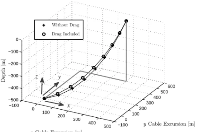
In Fig. 4, two cable profiles are presented. The first system, denoted by ‘+’ is modeled without drag forces. This geometry is solved using the procedures given by Eqs. 7–10 and constitutes as the reference pose. A solution is achieved in seven ǫ iterations. The second line, noted by the ‘◦’ symbol, is the final solution to the static problem with drag forces. This solution is achieved in 33 inner loop ǫ iterations. As expected, including drag effects results in an increase in the computational effort. A dynamics simulation was performed to confirm these results indeed constitute a statics solution.
Interestingly, as the number of nodes is increased, the shooting method will converge onto a solution with less iterations. Increasing the resolution of the ca-ble has the effect of making the initial estimates for Hx′ and V from Eqs. 6a–6b
more accurate for the lumped mass cable. In comparison, the alternative conven-tional approaches were not as efficient. For the identical demonstrated case, the incremental method converged only after approximately 17,000 iterations, with
AE0 = 90000 Newtons and A∆E = 10000 Newtons. The dynamic relaxation ap-proach could not achieve a desirable solution after 70,000 time steps. Both cases used positions along the continuous cable defined by Eqs. 6a–6b as initial guesses. Webster (1980) demonstrates the use of an adaptively varied damping coefficient to promote convergence, which is not included in our implementation. A similar scheme introduced by Wu (1995) achieves convergence in 14 to 230 time steps; however, the number of time steps required depends greatly on the accuracy of the initial guess, and efficiency decreases as cable resolution increases.
−100 0 100 200 300 400 500 −100 0 100 200 300 400 500 600 −500 −400 −300 −200 −100 0 yCable Excursion [m] xCable Excursion [m] D ep th [m ] Without Drag Drag Included y x z
FIG. 4. Profile for a cable in a vacuum (+) and for a system subjected to an Um = 2 m/s ocean current (o). Thirty–three ǫ iterations are needed to achieve convergence for the case with hydrodynamic forces.
Alternative Initial Conditions
The examples studied so far consider problems where the first and final node positions are defined, but shooting method can be amended to solve problems where other boundary conditions are prescribed. For instance, consider the fol-lowing conceptual problem: a cable is pinned at its bottom end at a known point. Its upper end is supported on a horizontal surface at heighth, but the upper node is free to slide on that surface. Known horizontal forces Hx and Hy are applied
at the upper node. With minor changes, this problem can also be solved using the shooting method. In this example, we select lx, ly and V as the variables
iterated in the numerical solver. The parameters minimized still remains to be Eq. 11 and, if drag is present, Eq. 18.
SHOOTING METHOD DEFICIENCIES
In some instances, the shooting method fails to converge onto a solution. For simplicity, these cases are identified by evaluating the condition number for a cable in two dimensions, (i.e., with drag forces not present), but these limitations also extend to conditions with drag as well. The condition number is evaluated at the final solution for Hx′ and V for varying location of the upper node position, r1. Identical cable properties defined from the previous example are retained for this exercise, except that lx′ and h are now varied. This procedure is followed to
produce Fig. 5.
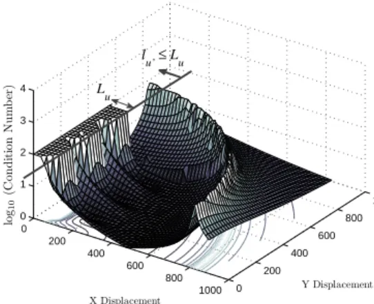
For the sake of clarity, the log10 of the condition number is plotted and a ceiling of 100 is applied in Fig. 5. The first zone of non–convergence forms a ridge around the origin. On either sides of the ridge, we encounter regions where convergence is likely. The second failure region is aligned parallel with thez–axis and is periodic in nature. The sources for these deficiencies will now be discussed in more detail.
First Region of Non–Convergence
The first region of ill–conditioning is identified by the circular ridge in Fig. 5. This non–convergence zone is concentric and at a distance ofL0 from the origin and marks the threshold where a cable transitions between taut and slack. In particular, when the cable has the same density as the surrounding fluid, points along L0 =
p l2
x+h2 do not converge. As the cable mass increases or decreases
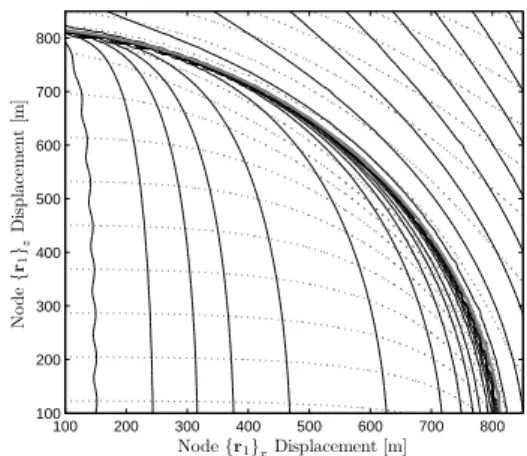
beyond this point, convergence is achieved with less trouble. This effect has direct implications when a solution is sought in a micro–gravity environment or in the case of synthetic cables in water, which can be neutrally buoyant. The source of this ill–conditioning region is attributed to the solver’s inability to resolve unique values forHx′ andV near the concentric ridge. As the net cable weight approach
zero, the system shows a high degree of sensitivity to small variations inHx′ and
V. Figure 6 below shows lines of constant and horizontal (Hx′) and vertical (V)
tension as a function of upper node displacement. The contour shows that, along the ridge where L0 =
p l2
x+h2, nearly identical values for Hx′ and V are used.
Further away from this region, the contour lines diverge from one another. The shooting algorithm operates most efficiently when vertical and horizontal contour lines are perpendicular to one another, and this coincides with regions identified by small condition numbers.
0 200 400 600 800 1000 0 200 400 600 800 1000 0 1 2 3 4 Y Displacement X Displacement log 1 0 (C on d it ion Nu m b er ) L u l u’≤ Lu
FIG. 5. Mapping of the condition numberJ as a function of the upper node displacement.
Second Region of Non–Convergence
The second region of non–convergence occurs when the cable has a sharp curvature - i.e., when it has a sharp ‘J’ or ‘U’ profile – and the element length is too long to smoothly follow the curvature. Figure 5 shows this region, which is spaced a maximum distance of Lu from the x–axis. Convergence becomes
problematic when:
lx′ ≤Lu (19)
Deficiencies are encountered when the unstretched element length is greater than the x distance between the first and final nodes. Problems occur because the
Node{r1}xDisplacement [m] No d e { r 1 }z D is p lac em en t [m ] 100 200 300 400 500 600 700 800 100 200 300 400 500 600 700 800
FIG. 6. Contours of constant tension: vertical force V (· · ·) and horizontal force Hx′ (–).
cable cannot round the curve at the base of the ‘J’ using the number of nodes identified, and signals that the cable resolution must be increased. This is fixed by increasing the number of elements n, thereby reducing Lu. Although increasing n mends the situation, enough nodes should be used to accurately represent the cable curvature.
Robustness Test
A robustness test is performed on the shooting method to evaluate its utility when a poor set of initial guesses are used. This test case is derived from Webster (1980), which is also used in Zueck (1995). Figure 7 illustrates the evolution of the solution using the shooting method, which is achieved in 23 iterations. In contrast, Webster requires 28 iterations, while Zueck’s techniques needs two iterations. If the initial starting profile is generated with Eqs. 6a–6b in mind, a total of nine iterations are needed with the shooting method. This test shows that the shooting method is an effective statics solution strategy when reasonable initial estimates are not known.
CONCLUSION
Approaches for solving the lumped mass cable statics configuration have been analyzed in this paper. Among the techniques touched on, the method of dy-namic relaxation is perhaps the most robust solution in terms of guaranteeing convergence. This method, however, can be very slow in cases where the cable is stiff (requiring small time steps) or if the required accuracy is high (i.e., accel-erations close to zero). The incremental method offers an alternative approach by using a Newton–Raphson algorithm to directly solve for the node positions along a cable. A disadvantage of this method concerns systems modeled with many nodes. As the number of nodes increases, the number of simultaneously solved equations increases proportionately. The rate of convergence decreases as the element stiffness increases.
−80 −60 −40 −20 0 20 40 60 80 −20 −15 −10 −5 0 5 10 15 20 X displacement [m] Y d is p lac em en t [m ] 2 4 6 8 10 12 14 16 18–23 Initial Guess Final Iteration
FIG. 7. Snapshot of the solution evolution with the shooting method using the cable properties defined by the exercise in Webster (1980).
A shooting algorithm was then described, and its effectiveness was demon-strated by modeling a cable in three dimensions subjected to fluid drag loading, which achieves a solution in 33 iterations. In general, the shooting algorithm serves as a more practical approach compared to dynamic relaxation or the incre-mental method since 1) it requires fewer iterations and 2) increasing the number of nodes has a beneficial effect. Regardless of the size ofn, the shooting algorithm must only minimize two equations for the three–dimensional problem, Eq. 11 and Eq. 18. This paper also discussed conditions when the shooting method may fail by analyzing a cable in two dimensions, though these same restrictions hold for the three dimensional case. In three–dimensions, non–convergence arises when
L0 =
p l2
x+ly2+h2 ≤Lu and serves as a warning that the cable resolution must
be increased to model the cable accurately. A second zone of non–convergence arises when L0 =
p l2
x+ly2+h2 and is analogous to the ridge formed in Fig. 6.
This non–convergence region becomes problematic when an equilibrium profile is sought for a neutrally buoyant cable. If convergence cannot be obtained with the current method, the options are: 1) relax the cable density by a small amount; 2) resort to the dynamic relaxation (or equivalent) method; or 3) approach the prob-lem using the “event–to–event” strategy outlined in Zueck (1995). The technique developed in this paper demonstrates an ability to attain convergence more effi-ciently than the adaptive dynamic relaxation methods (such as the one proposed in Wu), but is not quite as good the Zueck’s method. The shooting method, however, does show promise as a robust solver, even when bad initial guesses are supplied.
REFERENCES
Chai, T., Varyani, K., and Barltrop, N. (2002). “Three–dimensional lumped– mass formulation of a catenary riser with bending, torsion and irregular seabed iteraction effects.” Ocean Engineering, 29.
FIG. 8. Shooting method flow chart
De Zoysa, A. (1978). “Steady–state analysis of undersea cables.” Ocean Engi-neering, 5.
Driscoll, F. (1999). “Dynamics of a vertically tethered marine platform,” Phd thesis, University of Victoria, British Columbia, Canada.
Friswell, M. (1995). “Steady–state analysis of underwater cables.” J. Waterway, Port, Coastal, and Ocean Engineering, 121.
Gobat, J. (2002). “The dynamics of geometrically moored compliant systems,” Phd thesis, Massachusetts Institute of Technology / Woods Hole Oceanographic Institute, Cambridge, MA,.
Huang, S. (1994). “Dynamics analysis of three–dimensional marine cables.” J. Waterway, Port, Coastal, and Ocean Engineering, 21(6).
Irvine, M. (1992). Cable Structures. Dover Publications, Mineola, NY, USA. Kamman, J. and Huston, R. (1999). “Modeling of variable length towed and
tethered cable systems.” J. Guidance, Control, and Dynamics, 22(4).
Ketchman, J. and Lou, Y. (1975). “Application of the finite element method to towed cable dynamics.” Proceedings of MTS/IEEE OCEANS, Los Angeles, CA. 98–107. Vol. 1.
Malaeb, D. (1982). “Dynamic analysis of a tension leg platform,” Phd thesis, Texas A&M University, College Station, TX.
on nonlinear response of tlp.” J. Structural Engineering, 122(2).
Merchant, H. and Kelf, M. (1973). “Non–linear analysis of submerged buoy sys-tems.” Proceedings of MTS/IEEE OCEANS. 390–395. Vol. 1.
Nahon, M. (1999). “Dynamics and control of a novel radio telescope antenna.”
American Institute of Aeronautics and Astronautics.
Peyrot, A. (1980). “Marine cable structures.” J. Structural Division, ASCE, 106(12).
Powell, G. and Simons, J. (1981). “Improve iteration strategy for nonlinear struc-tures..” J. Numerical Methods in Engineering, 17, 1455–1467.
Shugar, T. (1991). “Automated dynamic relaxation solution method for compliant structures.” American Society of Mechanical Engineers, Annual Meeting of the American Society of Mechanical Engineers. 1–12. Vol. 4.
Strang, G. (1981). Linear Algebra and its Applications. Academic Press, Inc., New York, NY, USA.
Vesli´c, K. (1995). “Finite catenary and the method of lagrange.” Society for Industrial and Applied Mathematics, 37(2).
Walton, T. and Polacheck, W. (1960). “Calculation of transient motion of sub-merged cables.” Mathematics of Computation, 14(69).
Webster, R. (1980). “On the static analysis of structures with strong geometric nonlinearity.” Computers & Structures, 11.
Williams, P. and Trivaila, P. (2007). “Dynamics of circularly towed cable systems, part 1: Optimal configurations and their stability..”Journal of Guidance, Con-trol, and Dynamics, 30(2), 753–765.
Wilson, J. (2003).Dynamics of Offshore Structures. John Wiley & Sons, Hoboken, NJ.
Wu, S. (1995). “Adaptive dynamic relaxation technique for static analysis of catenary mooring..” Marine Structures, 8(5), 585–599.
Zueck, R. (1995). “Stable numerical solver for cable structures.” International Symposium on Cable Dynamics., Liege, Belgium. 19–21.