Spatial Patterns of Technology Di
ff
usion: An
Empirical Analysis Using TFP
Maria Abreu
∗Henri de Groot
†Raymond Florax
‡April 30, 2004
Abstract
We investigate the spatial distribution of TFP growth rates using ex-ploratory spatial data analysis and other spatial econometric techniques. Our sample consists of 73 countries and covers the period 1960-2000. We identify significant positive spatial autocorrelation in TFP growth rates, indicating that high and low values tend to be clustered in space. We alsofind strong positive spatial autocorrelation in TFP levels, which has increased over the period 1960-2000. This result may be indicative of a tendency towards clustering over time, a conclusion reinforced by our find-ing of two clusters of high TFP growth rates (in Europe and South East Asia), and two clusters of low TFP growth rates (in the Andean region and Sub-Saharan Africa). We estimate the Nelson and Phelps (1966) model of technology diffusion while allowing for spatial dependence in the error term. Our estimation results suggest that both the growth rate and the level of human capital have an important effect on productivity growth rates.
JEL:I2, O4, C21. Keywords: human capital, technology diffusion, spatial econometrics.
1
Introduction
Is there a spatial dimension to the flow of technology across country borders? Our aim is to investigate this question using exploratory spatial data analysis and other spatial econometric techniques. Following Coe and Helpman (1995), Keller (2001), Benhabib and Spiegel (1994, 2002) and others we study the effect of knowledge spillovers on Total Factor Productivity (TFP).
There are two broad schools of thought in the literature on the diffusion of technology across countries. The first one emphasizes the importance of absorptive capacity, that is, the ability of nations to adopt foreign technology for use in the domestic market. This view is based on the idea that there is a common pool of knowledge to which all countries have access, so that technology diffusion is constrained only by the receiving country’s ability to understand and make use of the new technology. A prominent example of this view is the Nelson
∗Department of Spatial Economics, Vrije Universiteit Amsterdam, De Boelelaan 1105, 1081
HV Amsterdam, The Netherlands ([email protected]).
†Vrije Universiteit Amsterdam and Tinbergen Institute. ‡Vrije Universiteit Amsterdam.
and Phelps (1966) model. The rate of adoption of new technology depends on the capacity of individuals and firms to implement new ideas, and on the gap between the technology they are currently using and the state of the art. The determinant of absorptive capacity in this case is the level of education.
Several empirical studies have found evidence in support of the absorptive capacity view. Benhabib and Spiegel (1994) use a growth accounting method to study the effect of human capital on productivity growth, andfind that human capital has a positive and statistically significant effect when interacted with the technology gap (as in Nelson and Phelps, 1966). Eaton and Kortum (1996)
find that inward technology flows (measured by patent citations) is increasing in the level of human capital. Xu (2000)finds that richer countries benefit from hosting US multinational subsidiaries while poor countries do not benefit as much, and that the discrepancy can be explained in terms of the level of human capital in the host country.
Absorptive capacity may also depend on the level of domestic R&D, so that domestic innovation must already have reached a critical level before foreign technology can be successfully adopted. Cohen and Levinthal (1989) show that
firms need to substantially invest in R&D in order to understand and evaluate new technological trends and innovations. Griffith, Redding and Van Reenen (2000)find that TFP growth is negatively correlated with the productivity gap (to the technology leader), particularly when the productivity gap is interacted with the level of domestic R&D.
Institutions may also influence absorptive capacity, an idea highlighted by the literature on innovation systems (Acs and Varga, 2002). Government poli-cies to promote research, networks of scientists and and good universities all encourage R&D and the adoption of foreign technology. Parente and Prescott (2000) argue that while technology is global, countries differ in theirresistance
to adopt new technologies, due to the excessive influence of domestic lobbies and state bureaucracies.
The second view on technology diffusion across countries emphasizes the importance of bilateral ties. Countries have different stocks of knowledge, and diffusion occurs through bilateral channels such as trade and Foreign Direct Investment (FDI). In general two mechanisms have been identified: (1) direct learning about foreign technology, and (2) employing specialised and advanced intermediate products developed abroad.
Direct learning requires a channel of communication between the two parties, especially since some knowledge may be tacit in that it cannot be codified and can only be passed from one person to another (Polanyi, 1958). There is some evidence that non-codified knowledge has a localised pattern: Feldman and Lichtenberg (1997) construct a measure of the tacitness of knowledge for a study of R&D activities in the EU. They find that the degree of tacitness of knowledge has an effect on the location of R&D activities.
Codified forms of knowledge (patents, blueprints, articles in scientific jour-nals) may also have a localised pattern. Eaton and Kortum (1996) study patent-ing activity in the OECD, andfind that patent citations decline with geograph-ical distance (although this finding may be due to the importance of within-country citations). Jaffe and Trajtenberg (2000) also find that intra-national spillovers (measured by patent citations) are larger than those between coun-tries. Part of this effect may be due to the sharing of a common language: Keller (2001)finds that bilateral language skills explain about 16% of bilateral
technology diffusion.
Direct learning in the form of tacit knowledge or via blueprints and arti-cles can be described as active technology diffusion (Keller, 2002). The other mechanism, known as passive diffusion, is the purchase and use in production of intermediate goods with embodied foreign knowledge. It is still a form of knowl-edge transfer, because it allows the buyer to implicitly use foreign technology in production. It may also encourage further domestic innovation through reverse engineering, or because it facilities domestic R&D (e.g. imports of computer equipment).
The empirical literature on technological diffusion has focused on trade and FDI. Coe and Helpman (1995) study the impact of trade on technology diffusion, and find that international R&D spillovers are related to the composition of imports (whether imports originated in high or low technology countries) and that the overall level of imports is also important. Eaton and Kortum (1996) and Keller (1998) provide evidence to suggest that import composition may not matter much once distance has been accounted for. Xu and Wang (1999) show that the import composition effect is robust when one considers trade in capital goods only instead of trade in all manufacturing goods. Keller (2001)finds that 69% of bilateral technology diffusion can be explained by trade patterns (and trade can be shown to be a function of bilateral distance).
In short, the empirical literature has found considerable evidence to suggest that technology diffusion may follow a spatial pattern, and that country char-acteristics such as the stock of human capital and the level of domestic R&D affect the rate at which a country adopts foreign technology. We commbine the two approaches by modifying the Nelson and Phelps (1966) model to allow for spatial dependence in TFP growth rates. Spatial econometrics techniques allow us to identify the type of spatial dependence present in the model and to estimate it consistently. Moreover, spatial data analysis techniques allow us to identify clusters and other anomalies such as spatial outliers, and to present the results visually in the form of Moran scatterplots and Moran significance maps. Spatial econometrics has mainly been used in applications at the level of re-gions, with several authors applying the techniques to income levels and growth rates, mostly in the context of models of income convergence. Rey and Montouri (1999) study income convergence among the states of the US over the period 1929-1994, andfind strong patterns of global and local spatial autocorrelation, with some evidence that temporal changes in spatial autocorrelation are associ-ated with changes in regional income dispersion. Mossi et al. (2003) use spatial data analysis techniques and Markov transition matrices to study growth and inequality in the regions of Brazil. They find evidence of the existence of two spatial clusters: a low income one in the Northeast and a high-income one in the Southeast. Lopez-Bazo et al. (1999), Le Gallo et. al (2003) and Fingleton (1999) apply spatial econometric tools to the analysis of the convergence in the European regions, andfind evidence of spatial dependence and clustering.
Studies at the country level are scarce. Moreno and Trehan (1997) use two different measures of distance: geographical distance and trade. Theyfind that a country’s growth rate is closely related to that nearby countries, and that trade alone cannot explain the spatial dependence. Ramírez and Loboguerrero (2002) apply spatial data analysis techniques to a sample of 98 countries over three decades (1965-75, 1975-85, 1985-95) and estimate a spatial dependence model that includes a number of political, economic and social variables.
There has, to our knowledge, been no spatial econometric analysis of TFP, either at the regional or country level.
The remainder of the paper is organised as follows. Section 2 describes our data set, and the method used to construct our measure of TFP. In section 3 we apply spatial data analysis techniques to investigate overall spatial patterns in the data, and the presence of clusters and outliers. Section 4 discusses the Nelson and Phelps (1966) model, and alternative specifications that allow for spatial dependence. Section 5 presents our empirical results, and section 6 concludes.
2
Data
We constructed our measure of TFP using a constant returns to scale Cobb-Douglas production function, with the capital share of income set to 1/3 and the labour share set to 2/3. Gollin (2002) shows that these are reasonable estimates, given that the share of labour lies between 0.65 and 0.85 for a large cross-section of developed and developing countries. We then calculated TFP as a residual:
lnT F Pit= lnYit− 1
3lnKit− 2
3lnLit (1)
whereYitis real output in countryiand timet;Kitis the capital stock andLit
is the total number of workers.
Our capital stock series was constructed using the perpetual inventory method: Kit=
t X j=0
(1−δ)t−jIij+ (1−δ)tKi0 (2)
where Iit is aggregate investment in physical capital in country i and time t
and δ is the rate of depreciation. An estimate of the initial capital stock was obtained from the expression for the capital/output ratio in the steady state:
Ki0
Yi0
= (I/Y)i
γ+δ+ni
(3) where Yi0 output in 1960; (I/Y)i is the investment share of output; γ is the
growth rate of output per capita in the steady state andni is the rate of
pop-ulation growth. Following Mankiw, Romer and Weil (1992) we assume a fixed value ofγ+δ, although in our case we assumeγ= 0.02andδ= 0.07, a higher depreciation rate (in line with recent estimates from microeconomic studies). We used 1960-1965 averages of the investment share and the population growth rate. The investment data is taken from PWT 6.1, using the real share of investment in GDP multiplied by GDP in constant PPPs.
For robustness we also tried varying the initial capital stock, the rate of depreciation (between 0.03-0.08), and the source of investment data (we also used the gross fixed capital formation series from the WDI 2002), all of which had little effect on the estimates. Our estimates of the capital stock are also highly correlated with more sophisticated series based on disaggregated data such as the PWT 5.6 capital stock series, Scarpetta et. al (2000) and Easterly and Levine (1999).
Our labour series is taken from PWT 6.1, and consists of the total number of workers. Our human capital data comes from the Barro and Lee (2001) dataset; we use the average years of schooling in the population aged 25 and over.
Our data covers a sample of 73 countries over the period 1960-2000 (see Table 1 in the appendix for a list of countries included in the analysis). Our sample is somewhat restricted for two reasons: (1) only countries whose borders did not change over the period can be included, this is because the weight matrix used in the spatial analysis is exogenously determined, and must remain constant over the whole period, (2) aggregate investment data is only available for a small sample of countries.
In Figure 1 we have plotted the growth rate of TFP over the period 1960-2000 against the logarithm of TFP in 1960. The result is a pattern frequently found in the literature. There is a slight negative correlation, indicating some tendency towards convergence in TFP levels. Figure 2 shows a scatter plot of the growth rate of TFP against the logarithm of schooling in 1960. In this case the correlation is more pronounced and positive, consistent with the hypothesis that higher schooling encourages technology transfer (as measured by TFP).
The spatial distribution of TFP growth rates can also be seen in Figure 3. Countries with high TFP growth rates over this period are Korea, Thailand, Japan, Ireland, Pakistan, Greece, Gabon, Portugal, Spain and Italy. Note the contrast with the distribution in Figure 4, showing the logarithm of TFP in 1960. There is some evidence that countries that lagged behind in terms of TFP in 1960 experienced rapid TFP growth over the period 1960-2000.
A similar pattern is apparent when comparing Figure 5 and Figure 6, show-ing the spatial distribution of schoolshow-ing growth rates and schoolshow-ing in 1960, respectively. There is some evidence of clustering of schooling levels in Figure 6, particularly in Latin American and in Europe. A rapid improvement in the average years of schooling of the population is particularly visible in Africa, South Asia and South-East Asia.
3
Exploratory Analysis
Spatial autocorrelation can be defined as the coincidence of value similarity with locational similarity (Anselin, 2001). There is positive spatial autocorrelation when high or low values of a variable tend to cluster together in space, and negative spatial autocorrelation if high values are surrounded by low values and vice-versa. A standard measure for spatial autocorrelation is the Moran’s I statistic. For a variablexand time tit is given by:
It= n S0 n P i=1 n P j=1 wij(xi,t−µt) (xj,t−µt) n P i=1 (xi,t−µt)2 (4)
where xi,t is the observation for country i and timet; µt is the mean value of
variable x at time t; n is the number of countries and wij is one element of
the spatial weights matrix W and S0 is a scaling factor equal to the sum of
all the elements ofW. The spatial weights matrix contains information on the spatial interdependence of the countries in the sample, and in our case has been constructed as follows:
wij = d−ij1 if dij<2000miles (5)
wheredijis the distance between the centroids of countriesiandjin miles. The
critical cut-offdistance of 2000 miles implies that we expect all spatial interac-tions above this distance to be negligible. Intuitively, our matrix in constructed so that interactions between countries decline with distance. Our cut-off dis-tance of 2000 miles was chosen in order to restrict technology spillovers to coun-tries that are situated fairly close together in space e.g. in the same continent (as a reference, the distance from coast to coast of the US is approximately 2500 miles).
Table 2 lists Moran’s I statistic and associated z- and p-values for three variables: (1) TFP growth (1960-2000), (2) ln(TFP) in 1960 and (3) ln(TFP) in 2000. Larger than expected values of Moran’s I indicate positive spatial autocorrelation, while smaller than expected values indicate negative spatial autocorrelation. Inference is (in our case) based on the normal approximation. In all three cases the z-value for Moran’s I is positive and significant, indicat-ing the presence of positive spatial autocorrelation. Intuitively, similar values (either high or low) are more spatially clustered than could have been caused by chance. The statistic is higher for TFP in 2000 than in 1960, indicating that TFP levels are becoming more clustered over time (consistent with theories of convergence clubs). Note also that TFP levels are more spatially autocorrelated than TFP growth rates.
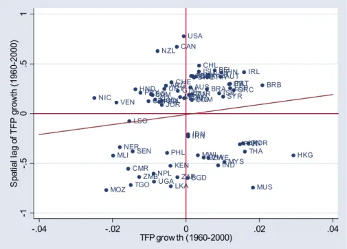
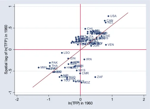
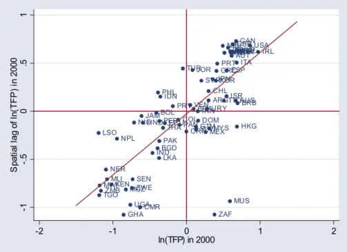
These results can also be seen visually by means of a Moran scatterplot (Anselin, 1996), which plots the spatial lagW zagainstz, wherezis the vector of observations for variablexin deviations from the meanµ. Moran’s I is formally equivalent to the slope coefficient of the linear regression ofW zonz, using a row-standardised weights matrix (a matrix is row-row-standardised when the elements wij in each row sum to 1). Figures 7, 8 and 9 are Moran scatterplots for the
variables TFP growth, ln(TFP) in 1960 and ln(TFP) in 2000 respectively. The four quadrants in the plot provide a classification of the observations into four types of spatial association: high values located next to high values (upper right-hand corner), low values located next to low values (lower left-right-hand corner), high values located next to low values (lower right-hand corner), and low values located next to high values (upper left-hand corner).
Consider the scatterplot in Figure 7 for TFP growth rates over the period 1960-2000. The Moran’s I statistic in Table 1 already indicated a low degree of spatial autocorrelation, and this can be seen in the plot (the observations are fairly scattered). The slope of the fitted line corresponds to the value of the Moran’s I statistic. There are two interesting results: a significant number of African countries are situated in the lower left-hand corner of the plot (low values close to low values), while a number of European countries are located in the upper right-hand corner of the plot (high values close to high values).
The use of standardised variables allows us to compare Moran scatterplots over time, so Figures 8 and 9 are directly comparable. It is immediately apparent that (in contrast with Figure 7) most observations are located in the upper-right and lower-left quadrants, corresponding to high-high and low-low values, respectively. It is also apparent that the spatial distribution of TFP levels is becoming more polarised over time. While in Figure 8 there are four or five visible groups of countries with similar values, in Figure 9 there appear to be only two clubs at the two extremes of the spatial distribution, with most other countries scattered in between.
significant spatial clustering of similar values around a particular observation. For a row standardised weights matrix, the global Moran’s I equals the mean of the local Moran’s statistics. Since there is a link between the local indicators and the global statistic, local outliers are also associated with the countries that exert the most influence on the global statistic. Figure 10 is a map showing the countries with significant values of the Local Indicator of Spatial Association (LISA) for TFP growth rates. The colour code also indicates the quadrant in the Moran scatterplot to which these countries belong. There are two clusters of low-low values: one comprises the Andean countries and Central America, the other one several countries of Sub-Saharan Africa. There are also two high-high clusters: one in Europe (including Turkey), and one in South-East Asia. Note in particular that the European and Sub-Sahara African clusters were also visible on the Moran scatterplot of Figure 7.
4
Model Speci
fi
cation
4.1
The Nelson-Phelps Model
In a seminal paper, Nelson and Phelps (1966) argue that the common practice of viewing education as simply another input in the production function should be ammended to take into account the observation that “educated people make good innovators”, by which they mean that education affects the speed at which new technologies are adopted. The authors make a distinction between the theoretical level of knowledge, or the cutting edge of technology, and the level of technology that prevails in practice. The theoretical level of knowledge is assumed to grow at a constant and exogenous rate:
Tt=T0eλt, λ >0 (7)
where Tt is the best attainable level of technology at time t. In this sense
their model is equivalent to the standard neoclassical model of growth, where the process creation of knowledge is exogenous, and technology is treated as a public good.
The rate at which theoretical knowledge is turned into improved technology in practice depends on the educational attainment of the adopters, and on the gap between the theoretical level of technology and the level of technology in practice: ˙ At At =Φ(h) · Tt−At At ¸ , Φ(0) = 0, Φ0(h)>0 (8) whereAtis the level of technology in practice andhis the level of educational
attainment. In the long run, the growth rate of technology in practice A(t) is equal to the growth rate of theoretical knowledgeTt, with a constant technology
gap.
Although the Nelson-Phelps model was developed with a view to explain technology adoption by individuals andfirms, there is a suggestion by the au-thors that the model might be applied to the study of economic growth. Ben-habib and Spiegel (1994) adapt the Nelson-Phelps model to study the effect of human capital levels in a growth accounting framework. To the Nelson-Phelps model in (8) the authors add an innovation term, arguing that in addition to the
successful adoption of foreign technology education also determines a nation’s capacity to develop new ideas. The growth rate of technology is given by:
˙ At At =g(h) +c(h) · Tt−At At ¸ (9) In order to estimate the model, they approximate the theoretical level of knowledgeTtby the level of technology in the technology leader (the maximum
level of TFP at time t), and assume that the level of educational attainment is constant over time (they use the average over the period). The level of educational attainment enters the equation in logarithmic form, so thatg(h) =
c(h) = ln(h). Their results broadly support the Nelson-Phelps model. The logarithm of human capital is found to have a statistically significant positive impact on productivity growth, both on its own and when interacted with the technology gap (Nelson-Phelps term). The authors also show that while the level of human capital is an important determinant of productivity growth, the growth rate of human capital is not. This result provides some evidence against the Lucas (1988) model of endogenous growth, where growth is driven by the accumulation of human capital.
We extend the Benhabib and Spiegel (1994) model of equation (9) in two ways. First, we allow the innovation term to depend on both the level and the growth rate of human capital, thus nesting the Nelson and Phelps (1966) and Lucas (1988) approaches. This allows us to test both approaches simultaneously. The distinction between the two models is important because they have very different implications for the effectiveness of investment in human capital. In the Lucas (1988) model, an increase in the level of human capital has a level effect on output, and long-run growth is only possible if human capital can grow without bound (for example, through improvements in the quality of schooling). In the Nelson and Phelps (1966) model an increase in the level of human capital increases the rate of innovation, and therefore has a growth effect on output. Our nested specification is the following:
˙ At At =α+β1ln(ht) +β2 ˙ ht ht +β3ln (ht) · max(At)−At At ¸ +u (10) whereu∼N(0, σ2I).
Note that we approximate the level of theoretical knowledge by the maximum level of technology at timet, and that human capital enters in logarithmic form. Second, we consider two types of econometric model to deal with the presence of spatial dependence: the spatial lag (or spatial autoregressive) model, and the spatial error model.
4.2
The Spatial Lag Model
In this model, the growth rate of technology in a country depends on several explanatory variables in that country (such as the human capital stock and the Nelson-Phelps term) and on the growth rate of technology in other countries located close to it in space. The extent of the spatial spillovers is given by the exogenously determined weights matrix W. The model in equation (10) becomes: ˙ At At =α+β1ln(ht) +β2h˙t ht +β3ln (ht) · max(At)−At At ¸ +ρWA˙t At +u (11)
whereu∼N(0, σ2I)andρis the spatial autoregressive parameter indicating the
extent of the interaction between observations according to the spatial pattern of the weights matrixW.
One important point to note is that this specification implies that the growth rate of technology in one country is affected by the explanatory variables in all other countries related to it by the spatial weights matrix. This can be seen by expressing the model in reduced form:
(I−ρW)A˙t At =α+β1ln(ht) +β2h˙t ht +β3ln (ht) · max(At)−At At ¸ +u (12) Rearranging: ˙ At At = (I−ρW)−1 " α+β1ln(ht) +β2 ˙ ht ht +β3ln (ht) · max(At)−At At ¸ +u # (13) Estimation of equation (11) by OLS results in biased and inconsistent es-timates, because the spatially lagged dependent variable is correlated with ε. Instead, the model can be estimated using instrumental variables or maximum likelihood (Anselin, 1988).
4.3
The Spatial Error Model
The spatial error model is a special case of the spatial lag model, with the spatial dependence restricted to the error term. Intuitively, we can think of the spatial dependence working through omitted variables with a spatial dimension (climate, social norms, exogenous shocks), so that the errors from different countries are spatially correlated. Equation (10) becomes:
˙ At At =α+β1ln(ht) +β2h˙t ht +β3ln (ht) · max(At)−At At ¸ +ε (14) ε=λW ε+u u∼N(0, σ2I)
whereλis a parameter indicating the extent of the spatial correlation between the regression residuals. Note that sinceε = (I−λW)−1u, the model can be rewritten as follows (compare with equation (13)):
˙ At At =α+β1ln(ht) +β2 ˙ ht ht +β3ln (ht) · max(At)−At At ¸ + (I−λW)−1u (15) Estimation of this model using OLS results in unbiased estimates of the parameter values, but biased estimates of the paramater variances. This model should therefore be estimated using maximum likelihood or general method of moments.
5
Empirical Findings
5.1
Standard Models
We start by estimating the standard model used by Benhabib and Spiegel (1994) given in equation (9). It has been suggested in the literature (Benhabib and Spiegel, 2002 and Engelbrecht, 2003) that the initial level of human capital (in our case ln(schooling) in 1960) may not be an adequate measure of the human capital available to countries in the spirit of the Nelson-Phelps model. The reason is that for a number of countries the stock of human capital in-creased dramatically over the period 1960-2000, and therefore the initial level does not reflect the amount of human capital available for innovation and adop-tion of foreign technology. We therefore estimate the model in equaadop-tion (9) using two different measures of the human capital stock: ln(schooling) in 1960, and ln(schooling) average over the period 1960-2000. Our data on human capi-tal is the average years of schooling in the population aged 25 and over, taken from the Barro and Lee (2001) dataset.
Column (1) in Table 3 shows the results of estimating the standard model, using ln(schooling) in 1960 as the measure of the human capital stock. The
coef-ficient of the Nelson-Phelps term (indicating technological catch-up) is positive as expected, and highly significant, indicating that countries that are further away from the technology leader experience higher productivity growth, given their levels of human capital stock. The effect of initial schooling on produc-tivity growth is also positive, although the estimated coefficient is fairly small (and not statistically significant at the 5% level). Roughly, the effect of a unit increase in ln(schooling) in 1960 (equivalent to about 2.72 years of schooling) results in an extra 0.08% growth in TFP.
Column (2) shows the results using average ln(schooling) over the period 1960-2000. The coefficient of the Nelson-Phelps term is again positive and highly significant, but also larger than in column (1). This could be an indication that the average years of schooling over the whole period are a better measure of the ability of countries to adopt foreign technology. The coefficient of ln(schooling) is again positive, but now also highly significant. The size of the effect of ln(schooling) on productivity growth is also larger, so that a unit increase in ln(schooling) (equivalent to 2.72 years of schooling) results in an extra 0.47% growth in TFP over the period. Our results confirm those of Benhabib and Spiegel (2002), who also find that using the period average of ln(schooling) results in larger coefficients for ln(schooling) and the Nelson-Phelps term. The
fit of the model in column (2) is also an improvement over that in column (1), as indicated by the higher values of the adjusted R-squared and F-statistic.
Column (3) shows the results of estimating model (10) with the restriction β1= 0, so that the innovation term is a function of human capital accumulation (as in the Lucas approach). The coefficient of the Nelson-Phelps term remains positive and highly significant, and has a larger value than in columns (1) and (2). The coefficient of schooling growth is also positive and significant at the 5% level. Roughly, an increase of 1% in the growth rate of schooling results in a 0.25% increase in the growth rate of TFP.
Column (4) shows the results of estimating the nested model of equation (10). Our aim with this specification was to test the relative merits of the Nelson and Phelps (1966) and Lucas (1988) approaches. Wefind that both the
growth rate of human capital and its level have a positive and significant impact on the growth rate of productivity. Interestingly, both coefficients are larger and more significant in the nested model than in the models where they appear on their own (columns (1) and (3)). A possible explanation is that the models in columns (1) and (3) suffer from omitted variable bias, since the growth rate and the level of schooling are highly (and negatively) correlated. Both variables have a positive impact on the growth rate of TFP, so omitting one or the other causes the coefficient of the remaining one to fall. It would seem that neither the Nelson and Phelps (1966) model or the Lucas (1988) model can fully explain the growth rate of TFP over the period 1960-2000.
The Jarque-Bera (1987) statistic does not reject normality for any of the models in Table 3, ensuring the validity of the spatial tests discussed below, and of the maximum likelihood estimation method used in Table 3. The White (1980) test for generic heteroscedasticity does not reject the null hypothesis of homoscedasticity for any of the models, but the Breusch-Pagan (1979) test is sig-nificant at the 5% level in columns (1) and (4), indicating that the residual vari-ance is correlated with one of the explanatory variables (most likely ln(schooling) in 1960). Since the tests for spatial dependence may beflawed in the presence of heteroscedasticity and vice-versa (Anselin and Griffith, 1988), we estimate a heteroscedatic error version of the model in column (4), using the following variables in the (additive) specification of the error variance: ln(schooling) in 1960, schooling growth, the Nelson-Phelps term, area in sqkm and population. These last two variables have been included because they are often found to be the cause of heteroscedasticity in cross-sectional models in the presence of spa-tial depedence (Anselin, 1988). The results are provided in column (1) of Table 4 (estimation is by feasible generalized least squares (FGLS)). The coefficients and standard errors remain mostly unchanged, indicating that the presence of heteroscedasticity had a minimal effect on the OLS results. Of the variables included in the additive error variance function, area in sqkm, population and ln(schooling) in 1960 were significant.
5.2
Spatial Diagnostics and Spatial Error Model
We consider five tests for spatial dependence. The test statistics are reported at the end of each column in Table 3. The first is Moran’s I test, adapted to regression residuals (Cliff and Ord, 1981). It is highly significant for all the models in Table 3, indicating the presence of spatial dependence. To discrim-inate between the two forms of spatial dependence outlined above (the spatial lag and spatial error model), we compare the lagrange multiplier (LM) test for spatial error and the LM test for spatial lag. Both are significant for all the models in Table 3, suggesting that the observed spatial dependence could take either form. The LM statistic for spatial error is larger in columns (1) and (3), while in columns (2) and (4) the LM statistics for spatial error and spatial lag are almost identical.
The robust LM tests for spatial error and spatial lag indicate the extent of spatial dependence of one form in the presence of spatial dependence of the other form. The statistics are very small and in most cases insignificant, reinforcing our previousfinding that the spatial dependence could take either form.
Given these results, we decide to focus on the spatial error model of equation (14) for the following reasons: (1) our nested specification seems the most
ap-propriate, because it avoids the possibility of omitted variable bias, and allows us to test between the Nelson and Phelps (1966) and Lucas (1988) models; (2) the LM statistic for spatial lag is slightly higher than the LM statistic for spatial error for the model in column (4), but the difference between the two values is very small; (3) the LM tests point to the spatial error model in all the other specifications; (4) the spatial error model is more realistic from a theoretical point of view, since we would not expect TFP growth in one country to be affected by all the explanatory variables in another country.
Column (2) of Table 4 shows the estimation results of the spatial error model of equation (14), corrected for heteroscedasticity using the same specification as in column (1). The spatially adjusted Breusch-Pagan statistic (Anselin, 1988) is not significant, indicating that the all the heteroscedasticity present in the OLS regression has been accounted for. As with the OLS regression in column (4) of Table 3, the coefficients of both the level and the growth rate of human capital are positive and significant, although their values have dropped slightly. The results now indicate that a 1% increase in the growth rate of schooling leads to a 0.50% increase in the TFP growth rate. The coefficient of the Nelson-Phelps term is positive and highly significant as before, and its value remains relatively unchanged. It should be noted that the estimate of the spatial error coefficient λ is positive and highly significant, indicating the presence of positive spatial autocorrelation. Two additional test statistics are provided. The likelihood ratio test for spatial error dependence is significant at the 5% level, indicating that the spatial error model provides a better fit than the standard regression model with the same set of explanatory variables (i.e. with λset to zero). The lagrange multiplier test for spatial lag dependence is not significant, indicating that the spatial error model has been correctly specified.
6
Conclusions
We have shown that TFP growth rates are spatially autocorrelated, so that high or low values tend to be clustered in space. There is also a significant amount of positive spatial autocorrelation in TFP levels, which appears to have increased over the period 1960-2000. We have used exploratory spatial data analysis techniques to investigate the presence of clusters in TFP growth rates, and have found two clusters of high values in Europe and South East Asia and two clusters of low values in the Andean region and Sub-Saharan Africa. Estimation of a standard model of technology diffusion such as the Nelson-Phelps results in autocorrelated residuals, and the standard spatial dependence tests indicate that a spatial error model would be more appropriate. We find that both the growth rate and the level of human capital have significant and positive impacts on the growth rate of TFP, and conclude that the Lucas (1988) and Nelson and Phelps (1966) approaches both contribute to explaining the evolution of productivity levels over time. One possibility that could be explored further is that both approaches might apply, if we were to distinguish between different types of human capital. The Nelson and Phelps (1966) model is related to the notion of absorptive capacity, and it might be more appropriate to consider only tertiary education and specialised training. The Lucas (1988) model, on the other hand, might be more related to the raising of basic educational levels across the population.
References
Acs, Z. & A. Varga (2002), ‘Geography, endogenous growth and innovation’,
International Regional Science Review26(2), 153—66.
Anselin, L. (1988), Spatial Econometrics: Methods and Models, Kluwer, Dor-drecht.
Anselin, L. (1996), The moran scatterplot as an esda tool to assess local in-stability in spatial association, in M.Fisher, H.Scholten & D.Unwin, eds, ‘Spatial Analytical Perspectives on GIS’, Taylor & Francis, London. Anselin, L. (2001), Spatial econometrics, in B.Baltagi, ed., ‘Companion to
Econometrics’, Basil Blackwell, Oxford.
Anselin, L. & D. Griffith (1988), ‘Do spatial effects really matter in regression analysis?’,Papers in Regional Science 74, 143—52.
Barro, R. & J. Lee (2001), ‘International data on educational attainment: Up-dates and implications’,Oxford Economic Papers3, 541—63.
Benhabib, Jess & M. Spiegel (2002), ‘Human capital and technology diffusion’,
Unpublished manuscript.
Benhabib, Jess & Mark M. Spiegel (1994), ‘The role of human capital in eco-nomic development: Evidence from aggregate cross-country data’,Journal of Monetary Economics34, 143—173.
Breusch, T. & A. Pagan (1979), ‘A simple test for heteroskedasticity and random coefficient variation’,Econometrica47, 1287—94.
Cliff, A. & J. Ord (1981), Spatial Processes: Models and Applications, Pion, London.
Coe, D. & E. Helpman (1995), ‘International r&d spillovers’, European Eco-nomic Review39, 859—87.
Cohen, W. & D. Levinthal (1989), ‘Innovation and learning: the two faces of r&d’,Economic Journal99, 569—96.
Easterly, W. & R. Levine (2002), ‘It’s not factor accumulation: Stylized facts and growth models’,Working Paper Central Bank of Chile91(164). Eaton, J. & S. Kortum (1996), ‘Trade in ideas: Patenting and productivity in
the oecd’,Journal of International Economics40, 251—78.
Engelbrecht, H. (2003), ‘Human capital and economic growth: Cross-section evidence for oecd countries’,Economic Record79, 40—51.
Feldman, M. & F. Lichtenberg (1997), ‘The impact and organization of publicly-funded r&d in the european community’,NBER Working Paper 6040. Fingleton, B. (1999), ‘Estimates of time to economic convergence: An analysis
of regions of the european union’, International Regional Science Review
Gollin, D. (2002), ‘Getting income shares right’, Journal of Political Economy
110, 458—74.
Griffith, R., S. Redding & J. Van Reenen (2000), ‘Mapping two faces of r&d: Productivity growth in a panel of oecd industries’,Institute for Fiscal Stud-ies Working Paper #2000-2.
Jaffe, A. & M. Trajtenberg (2000), ‘International knowledge flows: evidence from patent citations.’,Economics of Innovation and New Technology. Jarque, C. & A. Bera (1987), ‘A test for normality of observations and regression
residuals’,International Statistical Review55, 163—72.
Keller, W. (1998), ‘Are international r&d spillovers trade related? analyzing spillovers among randomly matched trade partners’, European Economic Review42, 1469—81.
Keller, W. (2001), ‘The geography and channels of diffusion at the world’s tech-nology frontier’,NBER Working Paper Series92(8150).
Keller, W. (2002), ‘International technology diffusion’,CEPR Discussion Paper Series92(3133).
Le Gallo, J., C. Ertur & C. Baumont (2003), A spatial econometric analysis of convergence across european regions, 1980-1995, in B.Fingleton, ed., ‘European Regional Growth’, Springer, Berlin.
López-Bazo, E., E. Vayá, A. Mora & J. Suriñach (1999), ‘Regional economic dy-namics and convergence in the european union’,Annals of Regional Science
33, 343—70.
Lucas, R. (1988), ‘On the mechanics of economic development’,Journal of Mon-etary Economics22, 3—24.
Moreno, R. & B. Trehan (1997), ‘Location and the growth of nations’,Journal of Economic Growth2(4), 399—418.
Mosi, M., P. Aroca, I. Fernandez & C. Azzoni (2003), ‘Growth dynamics and space in brazil’,International Regional Science Review26, 393—418. Nelson, R. & E. Phelps (1966), ‘Investment in humans, technological diffusion,
and economic growth’,American Economic Review56(1/2), 65—75. Parente, S. & E. Prescott (2000), Barriers to Riches, MIT Press, Cambridge,
MA.
Polanyi, M. (1958), Personal Knowledge: Towards a Post-Critical Philosophy, University of Chicago Press, Chicago.
Ramírez, M. & A. Loboguerrero (2002), ‘Spatial dependence and economic growth: Evidence from a panel of countries’,Banco de la República, Colom-bia33.
Rey, S. & B. Montouri (1999), ‘Us regional income convergence: A spatial econometric perspective’,Regional Studies33(2), 143—56.
Scarpetta, Bassanini, Pilat & Schereyer (2000), ‘Economic growth in the oecd area: Recent trends at the aggregate and sectoral level’,OECD Economics Department Working Papers98(248).
White, H. (1980), ‘A heteroskedastic-consistent covariance matrix estimator and a direct test for heteroskedasticity’,Econometrica48, 817—38.
Xu, B. (2000), ‘Multinational enterprises, technology diffusion, and host country productivity growth’,Journal of Development Economics62, 477—493. Xu, B. & J. Wang (1999), ‘Capital goods trade and r&d spillovers in the oecd’,
Canadian Journal of Economics32, 1258—74.
A
Tables and Figures
Table 1: Total Factor Productivity estimates
Country ISO code TFP growth ln(TFP) in 1960
Argentina ARG 0.0057 6.3508 Australia AUS 0.0123 6.4568 Austria AUT 0.0206 6.0663 Bangladesh BGD 0.0115 5.4228 Barbados BRB 0.0320 5.6936 Belgium BEL 0.0190 6.2358 Bolivia BOL 0.0016 5.8049 Brazil BRA 0.0169 5.6992 Cameroon CMR -0.0046 5.8287 Canada CAN 0.0086 6.6065 Chile CHL 0.0147 5.9919 Colombia COL 0.0045 5.9903
Costa Rica CRI 0.0009 6.2399
Denmark DNK 0.0138 6.3695
Dominican Rep. DOM 0.0127 5.9270
Ecuador ECU 0.0106 5.5571 El Salvador SLV 0.0027 6.2988 Finland FIN 0.0208 6.0684 France FRA 0.0169 6.2039 Ghana GHA 0.0160 4.7850 Greece GRC 0.0241 5.7204 Guatemala GTM 0.0089 6.0502 Honduras HND -0.0027 5.7931 Hong Kong HKG 0.0404 5.3483 Iceland ISL 0.0146 6.2577 India IND 0.0199 5.0205 Indonesia IDN 0.0117 5.4532 Iran IRN 0.0117 5.9634 Ireland IRL 0.0270 6.1730 Israel ISR 0.0201 6.0169 Italy ITA 0.0229 6.0445
Table 1: (continued)
Country ISO code TFP growth ln(TFP) in 1960
Jamaica JAM 0.0020 5.5867 Japan JPN 0.0267 5.5644 Jordan JOR 0.0045 6.1180 Kenya KEN 0.0069 4.9786 Lesotho LSO -0.0043 5.2542 Malawi MWI 0.0144 4.5224 Malaysia MYS 0.0216 5.7238 Mali MLI -0.0087 5.5467 Mauritius MUS 0.0294 5.6932 Mexico MEX 0.0095 6.1577 Mozambique MOZ -0.0106 5.8766 Nepal NPL 0.0023 5.2414 Netherlands NLD 0.0130 6.4407 New Zealand NZL 0.0034 6.6360 Nicaragua NIC -0.0139 6.1203 Niger NER -0.0069 5.4611 Norway NOR 0.0174 6.2090 Panama PAK 0.0258 4.8754 Pakistan PAN 0.0119 5.7067 Paraguay PRY -0.0013 6.1440 Peru PER 0.0038 5.7569 Philippines PHL 0.0060 5.6526 Portugal PRT 0.0232 5.7695 Senegal SEN -0.0034 5.6820
South Africa ZAF 0.0088 6.3081
South Korea KOR 0.0281 5.5505
Spain ESP 0.0232 5.8987
Sri Lanka LKA 0.0070 5.6249
Sweeden SWE 0.0133 6.3418
Switzerland CHE 0.0072 6.5056
Syria SYR 0.0213 5.6287
Thailand THA 0.0272 4.8727
Togo TGO -0.0039 5.2493
Trinidad & Tobago TTO 0.0127 6.2789
Turkey TUR 0.0128 5.7144
Uganda UGA 0.0024 5.4164
United Kingdom GBR 0.0125 6.4045
United States USA 0.0105 6.7208
Uruguay URY 0.0052 6.3493
Venezuela VEN -0.0079 6.6422
Zambia ZMB -0.0016 5.1815
Table 2: Moran’s I Statistics
Moran’s I Z-Value Probability
TFP growth (1960-2000) 0.2831 4.2419 0.0000
ln(TFP) in 1960 0.5770 8.4384 0.0000
ln(TFP) in 2000 0.6372 9.2986 0.0000
Table 3: Standard Models
(1) (2) (3) (4) Constant 0.0078** -0.0027 0.0019 -0.0121* (0.0016) (0.0023) (0.0032) (0.0052) Nelson-Phelps term 0.0259** 0.0377** 0.0429 0.0312** (0.0098) (0.0076) (0.0089) (0.0090) ln(schooling) in 1960 0.0008 0.0078** (0.0018) (0.0024) ln(schooling) average 1960-2000 0.0047** (0.0015) Schooling growth (1960-2000) 0.2506 0.6418** (0.1166) (0.1621) Observations 73 73 73 73 F statistic 10.58 26.68 13.44 13.76 adj. R-squared 0.21 0.42 0.26 0.35 Jarque-Bera 0.14 1.21 0.90 0.97 Breusch-Pagan test 8.24* 5.16 0.43 7.61* White 10.85 7.91 4.58 12.94 Moran’s I (error) 4.82** 4.10** 4.86** 3.04**
Lagrange multiplier (error) 13.93** 11.70** 13.39** 6.16**
Robust LM (error) 0.00 1.01 0.04 0.67
Lagrange multiplier (lag) 16.87** 11.92** 17.68** 5.77**
Robust LM (lag) 2.94 1.23 4.32* 0.29
Standard errors are in parentheses. ∗significant at 5%; ∗∗ significant at 1%. (1), (2), (3)
Table 4: Heteroscedastic and Spatial Models (1) (2) Constant -0.0110* -0.0073 (0.0048) (0.0053) Nelson-Phelps term 0.0351** 0.0345** (0.0070) (0.0097) ln(schooling) in 1960 0.0069** 0.0057* (0.0021) (0.0025) Schooling growth (1960-2000) 0.6375** 0.4921** (0.1440) (0.1563)
Lambda (spatial error) 0.3787**
(0.1459)
Observations 73 73
Breusch-Pagan / Spatial B-P 8.97
Moran’s I (error)
Lagrange multiplier (error) 19.81**
Robust LM (error)
Lagrange multiplier (lag) 18.61** 0.13
Robust LM (lag)
Likelihood ratio (error) 5.39**
Standard errors are in parentheses. ∗ significant at 5%; ∗∗
significant at 1%. (1) heteroscedastic error model estimated using FGLS; (2) spatial error model estimated using ML.
Figure 1: Scatter of TFP growth (1960-2000) against ln(TFP) in 1960 ARG AUT AUS BRB BGD BEL BFA BDI BEN BOL BRA CAN COG CHE CIV CHL CMR CHN COL CRI CPV DNK DOM ECU EGY ESP ETH FIN FRA GAB GBR GHA GMB GIN GRC GTM GNB HKG HND IDN IRL ISR IND IRN ISL ITA JAM JOR JPN KEN COM KOR LKA LSO LUX MAR MDG MLI MUS MWI MEX MY S MOZ NER NGA NIC NLD NOR NPL NZL PAN PER PHL PAK PRT PRY ROU RWA SY C SWE SEN SLV SY R TCD TGO THA TUR TTO TZA UGA USA URY VEN ZAF ZMB ZWE -. 02 0 .0 2 .0 4 T F P g row th ( 196 0-20 00) 4 5 6 7 ln(TFP) in 1960
Figure 2: Scatter of TFP growth (1960-2000) against ln(schooling) in 1960
ARG AUT AUS BRB BGD BEL BOL BRA CAN CHE CHL CMR COL CRI DNK DOM ECU ESP FIN FRA GBR GHA GRC GTM HKG HND IDN IRL ISR IND IRN ISL ITA JAM JOR JPN KEN KOR LKA LSO MLI MUS MWI MEX MY S MOZ NER NIC NLD NOR NPL NZL PAN PERPHL PAK PRT PRY SWE SEN SLV SY R TGO THA TUR TTO UGA USA URY VEN ZAF ZMB ZWE -. 02 0 .0 2 .0 4 T F P g row th ( 19 60 -2 000) -3 -2 -1 0 1 2 ln(schooling) in 1960
Figure 3: Distribution of TFP growth rates (1960-2000) -0.014 - 0.002 0.002 - 0.009 0.009 - 0.013 0.013 - 0.021 0.021 - 0.04 Figure 4: Distribution of ln(TFP) in 1960 4.522 - 5.453 5.453 - 5.714 5.714 - 6.044 6.044 - 6.279 6.279 - 6.721
Figure 5: Distribution of schooling growth rates (1960-2000) 0.003 - 0.009 0.009 - 0.014 0.014 - 0.02 0.02 - 0.03 0.03 - 0.082
Figure 6: Distribution of ln(schooling) in 1960
-2.604 - 0.334 0.334 - 0.892 0.892 - 1.405 1.405 - 1.754 1.754 - 2.257
Figure 7: Moran scatterplot of TFP growth (1960-2000) (note: both axis are in deviations from the mean)
ARG AUS AUT BRB BEL BGD BOL BRA CAN LKA CHL CMR COL CRI DNK DOM ECU IRL SLV FIN FRA GHA GRC GTM HKG HND ISL IDN IND IRN ISR ITA JPN JAM JOR KEN KOR LSO MWI MLI MUS MEX MYS MOZ NER NLD NOR NPL NIC NZL PRY PER PAK PAN PRT PHL ZAF SEN ESP SWE SY R CHE TTO THA TGO TUR UGA GBR USA URY VEN ZMB ZWE -1 -. 5 0 .5 1 S pat ia l l ag of T F P g row th ( 196 0-20 00 ) -.04 -.02 0 .02 .04 TFP grow th (1960-2000)
Figure 8: Moran scatterplot of ln(TFP) in 1960 (note: both axis are in devia-tions from the mean)
ARGAUS AUT BRB BEL BGD BOL BRA CAN LKA CHL CMR COL CRI DNK DOM ECU IRL SLV FIN FRA GHA GRC GTM HKG HND ISL IDN IND IRN ISR ITA JPN JAM JOR KEN KOR LSO MWI MLI MUS MEX MY S MOZ NER NLD NOR NPL NIC NZL PRY PER PAK PAN PRT PHL ZAF SEN ESP SWE SY R CHE TTO THA TGO TUR UGA GBR USA URY VEN ZMB ZWE -1 -. 5 0 .5 1 S pat ia l l ag of ln (T F P ) i n 19 60 -2 -1 0 1 2 ln(TFP) in 1960
Figure 9: Moran scatterplot of ln(TFP) in 2000 (note: both axis are in devia-tions from the mean)
ARG AUS AUT BRB BEL BGD BOL BRA CAN LKA CHL CMR COL CRI DNK DOM ECU IRL SLV FIN FRA GHA GRC GTM HKG HND ISL IDN IND IRN ISR ITA JPN JAM JOR KEN KOR LSO MWIMLI MUS MEXMYS MOZ NER NLD NOR NPL NIC NZL PRY PER PAK PAN PRT PHL ZAF SEN ESP SWE SY R CHE TTO THA TGO TUR UGA GBR USA URY VEN ZMB ZWE -1 -. 5 0 .5 1 S pat ia l l ag of ln (T F P ) i n 20 00 -2 -1 0 1 2 ln(TFP) in 2000
Figure 10: LISA cluster map for TFP growth rates (1960-2000)
Low-Low Low-High High-Low High-High