Does Tariff Liberalization Increase Wage Inequality? Some Empirical Evidence

Full text

(1)NBER WORKING PAPER SERIES. DOES TARIFF LIBERALIZATION INCREASE WAGE INEQUALITY? SOME EMPIRICAL EVIDENCE Branko Milanovic Lyn Squire Working Paper 11046 http://www.nber.org/papers/w11046 NATIONAL BUREAU OF ECONOMIC RESEARCH 1050 Massachusetts Avenue Cambridge, MA 02138 January 2005. The work was in part financed out of World Bank Research Grant PO85725 (project on Globalization and Middle Classes). Milanovic would also like to acknowledge the support of McArthur Foundation. The paper is forthcoming in the book “Globalization and Poverty” edited by Ann Harrison (University of Chicago Press). The authors are grateful to Gouthami Padam for assistance with data collection, and to Ann Harrison, Doug Irwin, and participants of two National Bureau of Economic Research conferences for their comments and suggestions. The views are authors’ own and should not be attributed to the orgnaizations with which they are affiliated. The views expressed herein are those of the author(s) and do not necessarily reflect the views of the National Bureau of Economic Research. © 2005 by Branko Milanovic and Lyn Squire. All rights reserved. Short sections of text, not to exceed two paragraphs, may be quoted without explicit permission provided that full credit, including © notice, is given to the source..

(2) Does Tariff Liberalization Increase Wage Inequality? Some Empirical Evidence Branko Milanovic and Lyn Squire NBER Working Paper No. 11046 January 2005 JEL No. F1, F13, D31, J31 ABSTRACT The objective of the paper is to answer an often-asked question : if tariff rates are reduced, what will happen to wage inequality ? We consider two types of wage inequality : between occupations (skills premium), and between industries. We use two large data bases of wage inequality that have become recently available and a large dataset of average tariff rates all covering the period between 1980 and 2000. We find that tariff reduction is associated with higher inter-occupational and inter-industry inequality in poorer countries (those below the world median income) and the reverse in richer countries. The results for inter-occupational inequality though must be treated with caution. Branko Milanovic World Bank and Carnegie Endowment for International Peace 1779 Massachusetts Avenue, NW Washington, DC 20036 [email protected] Lyn Squire Global Development Network 2600 Virginia Avenue, NW Suite 1112 Washington, DC 20037 [email protected].

(3) 1. Introduction The relationship between globalization and the distribution of income remains a hotly debated issue in part because the link is complex and commingled with many other factors. In these circumstances, careful specification of the issue is essential. Theory offers the natural place to search for precision. And indeed theory does provide well specified analyses leading to apparently unambiguous predictions.. The standard. theoretical framework is the two-factor, two-county Heckscher-Ohlin model. In this model, trade liberalization will increase the relative price of the abundant factor which is usually taken to be unskilled labor in the case of developing countries. This in turn should reduce inequality.. Thus, a well-specified question leads to an unambiguous. prediction. The Heckscher-Ohlin specification, however, is a drastic simplification of a complex phenomenon and relatively minor steps towards greater realism or a shift in focus towards different aspects of globalization complicate matters. To take just one example, Feenstra and Hanson (1996) focus on a different form of globalization: the transfer of production from developed to developing countries.. In their model, the wage gap. between skilled and unskilled workers in developing countries increases, pointing towards increased inequality.. Thus, plausible models can lead to quite different. predictions. Whenever theory leads to different predictions, empirical evidence is required to help choose among alternatives. The available empirical literature, however, does not lead easily to robust conclusions regarding the relationship between globalization and inequality. The combination of a complex phenomenon and data inadequacies renders empirical work both hazardous and partial. Different authors focus on different aspects of the phenomenon ranging from within-country wage-inequality to global inequality. They employ different specifications sometimes relating levels of openness to levels of inequality and sometimes relating changes in openness to changes in inequality. And various alternative definitions of key variables are used including the measure of. 3.

(4) openness with some authors using quantities (trade volumes or flow of FDI) and others using policies (tariff levels). The end result is that a careful interpretation of the existing literature requires attention to all these possible points of differences in the various studies. The primary purpose of this paper is to present the results of a new empirical investigation of the relationship between globalization and inequality, one that we hope addresses some of the concerns raised above. In this respect, the paper makes two contributions. First, it presents a simple analytical model that focuses on the element of income distribution that is most likely to be affected by globalization, namely, wage income. And second, it draws on a review of the existing empirical literature to identify preferred ways of specifying the empirical counterpart to our theoretical model. An important advantage of this approach is that abundant data are available on the distribution of wage income in various forms. A secondary purpose is to incorporate one aspect of globalization that has not been captured in the academic literature but is prominent in the popular press. The media and many governments often interpret globalization as something that happens in the global economy and affects different countries in different ways. To see this, imagine a country that does not change its trade policy over a period of years. And imagine that over the same period most other countries liberalize their trade policies and the global volume of trade increases. The question then is whether the observed “globalization” can affects inequality in the country that has not changed its trade policies. The answer is “yes” if the global expansion of trade reduces the export volumes or prices of the nonglobalizing country. In this scenario, the non-globalizing country not only fails to participate in the benefits of an expanding world volume of trade but actually sees a deterioration in its position compared with the pre-globalization era. In other words, it may be insufficient to focus on a country’s own liberalization efforts. It may be more appropriate to focus on those efforts relative to the efforts of major trading competitors. In this view, the direction of causation is from a worldwide phenomenon to inequality.. 4.

(5) The lack of attention to the media view in the academic literature is surprising since it is in fact an example of a well-known economic concept, namely, pecuniary externalities. The paper begins in Section 2 with a review of existing empirical work in two critical dimensions: domain and specification. Domain refers to the type of globalization (products, capital, or labor) and the type of inequality (global inequality between all individuals in the world, inequality between the countries, within-country inequality between individuals, or wage-inequality between wage-earners) under examination. It also refers to the locus of the study and whether it is a single-country or a multi-county study. Specification is of two types with variables being measured either in levels or in first differences. This subsection also deals with the important issue of interaction between policy variables and initial conditions. In Section 3, we present a simple, yet comprehensive, model of the equilibrium relationship between wage inequality and trade policy. Four categories of wages are examined: for skilled and unskilled labor; and for labor in protected and unprotected sectors. The model allows us to explore the ways in which trade liberalization affects the skill premium, the protection premium, and the union premium In Section 4 we discuss the variables on wage inequality and trade and labor liberalization that we use in the empirical part. The empirical model in Section 5 is estimated in two different ways that draw on two large sets of data on wage inequality. One is a database of Occupational Wages around the World (OWW) covering the period from 1983 to 1999 and more than 150 countries. The data were collected from the ILO sources (the October Inquiry), and then put together and analyzed by Richard Freeman and Remco Oostendorp (2000).2. The other is a database of inter-industrial wage. differences created by James Galbraith and associates. This University of Texas Inequality Project (UTIP) database covers on average about 90 countries annually over the period 1975-99.3. 2. The Occupational Wages around the World (OWW) database in available at www.nber.com.. 3. The data are available at http://utip.gov.utexas.edu/.. 5.

(6) 2. Review of the Empirical Literature As noted in the Introduction, the literature contains a diverse collection of empirical efforts to identify the relationship between globalization and inequality. This diversity plagues the interpretation of results and comparisons across studies but at the same time it provides a valuable source of material to guide the empirical specification of the model presented in Section II. We thus review the existing literature with the specific objective of determining the lessons for the estimation of out theoretical model. Our review covers 15 papers completed within the last ten years. Of these, six point to a positive relationship between the chosen measure of globalization and the chosen measure of inequality. That is, globalization increases inequality. Three indicate that globalization increases inequality in low-income countries. Five studies find no impact on inequality.. Only one paper points to declining inequality among the. “globalizing countries” including the OECD. In addition, two other papers (Freeman, 1995, and Richardson, 1995) provide reviews of the then existing empirical literature and conclude that trade liberalization has a positive (increasing) albeit modest impact on inequality. What is surprising about this quick summary is that none of the studies indicate declining inequality in low-income countries, the one region where standard theory predicts such an outcome. The choice, then, seems to be between no impact and increased inequality. Two qualifications are in order, however. First, the results are often quite fragile: small changes in specification or definition of variables can undermine statistical significance. And second, each of the 15 studies focuses by necessity on only one aspect of the relationship between globalization and equity. In principle, then, these apparently contradictory results could in fact be perfectly consistent. To explore this further, we examine the studies in each of three dimensions: domain, or the focus of the investigation; specification, especially whether estimates are levels on levels, or changes on changes; and variable selection, including the choice of variable to represent trade liberalization. At the end of our discussion of each dimension, we select our preferred option(s) for our subsequent empirical analysis.. 6.

(7) Domain Globalization in the majority of papers is defined as increased openness in trade policy. Only two papers (Milanovic, 2005a, and Behrmann, Birdsall and Szekely, 2003) look at capital account liberalization. None define globalization in terms of increased labor mobility.. And with respect to inequality, both global inequality (inequality. between all citizens in the world) and within-country inequality receive attention in the context of multi-country studies. Interestingly, there is also a significant group of studies that focus on wage-inequality, typically in the context of single-country studies exclusively in Latin America. Clark, Dollar and Kraay (2001) is a good example of a paper dealing with global inequality. They find that inequality between the population-weighted mean incomes of the globalizing countries has decreased substantially between 1975 and 1995. This reflects increases in average incomes in key developing countries (especially China) relative to the OECD average, so that population-weighted between-country inequality has fallen. At the same time, they point to rising within-country inequality for this group of countries but not enough to offset the (population-weighted) between-country decline. This appears to be a fairly firm result but does not of course incorporate the countries that have not globalized. Here, Clark, Dollar and Kraay point to decline and divergence. Since these are some of the poorest countries in the world, this is clearly a matter of concern. Nevertheless, they show that inequality worldwide has declined between the second half of the seventies and the second half of the nineties despite these disparate experiences. If, however, one looks at the world as a whole, the conclusions regarding the global inequality (inequality between all individuals) are not so firm. Milanovic (2005) finds a sharp increase between 1988 and 1993, and then a moderate decline during the next five-year period. Sala-i-Martin (2002) and Bhalla (2002) argue that global inequality has gone down although their approach which combines household survey and national accounts (GDP data) is questionable, and the results may be driven by a number. 7.

(8) of strong assumptions that, in the absence of sufficient data, the authors make. 4 Global inequality is an area of intense controversy, but it is worth stating, whatever the “correct” results, neither of these studies explores the issues of causality—that is, the link between increased globalization and global inequality. Within-country inequality is the subject of several papers and is the area where results are also unclear. An early example of a paper concerned with within-country inequality is that by Edwards (1997). He regresses the change in the Gini index between the 1970s and the 1980s on a dummy indicating whether or not a country had engaged in trade liberalization as measured by the average black-market premium or the average collected tariff ratio. He finds that trade reform did not significantly affect inequality. Other authors arriving at similar results albeit using different specifications, time periods, and data include Londono (2002) and Dollar and Kraay (2001). Barro (2000), however, finds that openness, as measured by trade volumes, is associated with higher levels of inequality in a panel of countries. He concludes: “Basically, the data reveal a long-term positive association between the levels of openness and inequality”. Other authors, again using different methods and variable definitions, concur. Spilimbergo, Londono, and Szekely (1999) and Lundberg and Squire (2003) also detect a link between openness and increased inequality. Reconciling these results is difficult because they cover different countries and time periods (and could therefore be reflecting different relationships) and because they use different specifications and variable definitions. One possibility that emerges from other work is that country categorization may be very important.. Several authors. (Ravallion, 2002, Milanovic 2005a, Savvides 1998) find that their preferred measure of openness increases inequality in low-income countries. Barro (2000) also finds the relationship more pronounced in poorer countries.. In Spilimbergo, Londono and. Szekely (1999, p.88) openness affects countries differently depending on their endowments: in capital-rich countries, openness reduces inequality while in countries with abundant skilled-labor, openness increases inequality. The authors argue that the 4. See Milanovic (2003).. 8.

(9) former effect is driven by reduction of capital rents, the latter effect, however, is consistent with Heckscher-Ohlin. The mix of countries in aggregate studies may therefore be the crucial factor leading to different results. Either way, this is a very significant result for two reasons. First, it runs counter to the prediction of conventional trade theory and raises obvious policy concerns. And second, it suggests that empirical work would benefit from some attempt to interact policy changes and initial conditions to capture the possibility of different effects at different levels of development, a point to which we return below. Wage-inequality is addressed by several authors in the context of Latin America. For example, Harrison and Hanson (1999) examine the extent to which the increase in wage-inequality in Mexico was associated with the 1985 trade reform. They find that the reform did play a part but that other factors including foreign direct investment, export orientation, and technological change were also important. Regarding Mexico, Robertson (2000) argues that trade liberalization and “labor flexibilization” led to an erosion of rents in protected industries (which in the case of Mexico were less-skilled) while foreign investments increased demand for highly-skilled labor. The two effects resulted in widening wage distribution. Beyer, Rojas and Vergara (1999) find a similar effect of trade reform on wage-inequality in Chile because skill-intensive, resourcebased industries expanded following liberalization.. Arbache, Dickerson and Green. (2003) find that following the extensive trade liberalization in Brazil in the 1990’s, average wage in the traded sector fell compared to the non-traded sector (even after adjusting for education, experience etc.), and that the only category that was spared a decline were the highly educated because the returns to education went up. Arbache, Dickerson and Green (2003) argue that these results are consistent with the erosion of rents in the traded sector in the wake of opening up, and complementarity between new technology brought in by globalization and skilled labor. A very important paper is the one by Behrman, Birdsall and Szekely (2003) who look at the impact of various policies (trade, financial liberalization, privatization, and tax reform) jointly or independently on wage differentials in Latin America during the 9.

(10) last twenty years. Its use of policy indicators (developed by the Inter-American Development Bank) rather than of outcomes is very similar to the approach we shall adopt here. Behrman et al. conclude that more liberal trade regimes did not have an impact on wage differentials between different education categories. But financial liberalization and high-technology exports in the context of a liberal trade regime, however, contributed to the rising inequality. They conclude (p. 30), “it is not increases in trade but changes in technology that are associated with growing wage gaps.” These studies suggest three overall conclusions. First, it is extremely important to investigate each country’s production structure, the pre-reform sectoral structure of protection, and the reduction in protection by sector in order to understand the impact of trade reform. Second, trade reforms are seldom undertaken in isolation. Most often, they come together, in a “package” with labor reforms. Disentangling the two effects—in addition to accounting for the effects of technological progress that may be nonneutral—is extremely difficult. Third, the impact of trade reform on wage inequality is likely to be modest if firms adapt to liberalization in a variety ways such as reducing excess profits and raising productivity as well as reallocating labor. Indeed, a study for Brazil finds no impact on wage inequality.. Although returns to college education. increased (Green and Dickerson, 2001), the share of college-educated workers in the total labor force was insufficient to influence overall inequality. Each of the possible combinations of types of globalization and inequality is an appropriate subject for research. Each provides valuable information in its own right. For our subsequent work, we follow the majority of other researchers in this field and focus on liberalization of trade rather than other aspects of globalization such as investment flows and labor migration, data for the latter being especially difficult to obtain. Globalization in products is also worthy of study because it affects far more countries than globalization in capital flows or labor flows. And as far as inequality is concerned, we select within-country, wage inequality for the theoretical and empirical reasons given in Section II and because this has been a focus of lots of literature reviewed here.. 10.

(11) Specification Turning to the econometric specification of the relationship to be estimated, we take two points from our review: first, although most researchers have regressed levels on levels, we believe that the work undertaken to date points to the importance of focusing on changes in both the dependent and explanatory variables; and second, several studies as well as our theoretical model suggest the impact of policy change depends on the level of development and that therefore interactive relationships need to be incorporated. The specification in most studies is a relationship between levels of inequality and levels of globalization. These studies generally have more success in finding statistically significant results.. Thus, the studies that find a negative impact of globalization on. inequality rely on regressions run in levels. For example, Barro (2000) regresses the Gini index on the share of trade in GDN. Lundberg and Squire (2003) regress the Gini index on the Sachs-Warner measure of openness. On the other hand, the studies that regress changes in inequality on changes in globalization have a much more difficult time finding significant results.. For example, Edwards (1997) uses the change in. inequality between the 1970s and the 1980s as his dependent variable and a dummy indicating whether a country undertook trade reform as his explanatory variable. Dollar and Kraay (2001) use the growth in the income of the bottom 20 percent and changes in trade volume.. Both sets of authors conclude that trade reform and/or changes in. openness have no impact on inequality. Interestingly, two papers undertake both levels-on-levels and changes-on-changes analyses. Milanovic (2002) finds that openness hurts poorer deciles in low-income countries when the analysis relates levels to levels, but funds no measurable effect when he switches to changes on changes. Similarly, Harrison and Hanson (1999) find that high industry tariffs are associated with greater wage inequality when they conduct the analysis in levels but not in changes. This suggests that either there is no relationship. 11.

(12) between changes in openness and changes in inequality, or the data are not sufficiently fine to capture such a relationship. This is an important observation because in our view changes-on-changes is the preferred specification. Globalization is presumably a dynamic concept and a continuing one.. Regressions of levels-on-levels, however, typically attempt to compare stable. points of equilibrium.. Consider this argument.. Define globalization for present. purposes as trade openness measured by trade policies. Now imagine two countries, one of which liberalized trade policy ten years ago while the other has literally just implemented its trade liberalization. One would imagine that resource reallocation, changes in factor prices, and other adjustments would have played out in the ten years following the reform in the first country, and the distribution of income would have arrived at a new stationary state. The relationship between policy and inequality could therefore be interpreted as an equilibrium. In the other country, however, trade policy will have changed but the economy, including inequality, will not have had a chance to adjust. If these two countries appear as two observations in a cross-country regression of levels on levels, it is very difficult to interpret the meaning of any results whether statistically significant or not. On the other hand, if the change in policy is related to the change in inequality after some common period of time in both countries, then the results, whatever they may be, are easily interpreted. With this argument in mind, we focus our empirical work on variables measured in first differences. That is, we focus on changes in countries’ policy stances and changes in inequality outcomes. A second point that emerges clearly from the review is that the impact of liberalization may differ depending on the initial conditions of the liberalizing country. However in the empirical work this approach is not always implemented. The implicit assumption is often that the effects of reforms are the same regardless of the initial level of policy openness or income. In other words, opening up an entirely closed economy by one reform point yields the same results as further opening of an already open economy. We shall try to avoid this type of simplification by controlling for the initial level of openness and income and, of course, for other initial differences between economies.. 12.

(13) Similarly, reforms which are each represented by one policy variable are seen, for econometric convenience, to affect outcomes additively. This is a strong simplification: reforms might often act multiplicatively in that the absence of one type of reform negates the effects of another. We shall try to allow for this by including interaction terms. 3. Trade and labor reforms, and wage inequality: an accounting model Model focus and justification In this section, we present a simple model of wage determination for four types of labor: skilled, unskilled; and labor employed in the protected and unprotected sectors. We also allow for different types of unionization: skill-based or sector-based. We focus the model in this way for two theoretical reasons and one empirical reasons. The first theoretical reason is that the link between policy reforms and wage inequality is likely to be much stronger than the link between policy reforms and inequality in total income. What happens to total income and its inequality is mediated by a number of other factors, including the role of social transfers (pension spending or family benefits), demographics of the population, family formation and mating, labor force participation, and so on. Since wage inequality is relatively immune to such factors, the link between policy and the distribution of wages should be much stronger than that between policy and the distribution of total income, and should therefore be easier to detect empirically. The second theoretical reason stems from the complexity of the relationship between policy and the distribution of wages in a country and how best to model it. Consider some of the puzzles and complexities that have been discussed in the recent literature. For example, a number of factors have been adduced to explain rising interoccupational inequality (or an increasing skill premium) following trade liberalizations in. 13.

(14) developing countries5. This is in direct contradiction to what one might expect based on the sample version of the Stolper-Samuelson theorem, namely that increased demand for low-skilled products (the alleged comparative advantage of poor countries) should increase relative wages of unskilled workers. Moreover, recent developments differ from those in the 1950’s and 1960’s when trade liberalization in Asian countries did produce the expected effect (Singh and Dhumale, 2000, p. 25; Arbache, Dickerson and Green 2003, p. 5). Some of the most popular explanations for increasing wage inequality in both poor and rich countries are the role of skill-biased technological progress (for a review see Slaughter, 1999; also Slaughter 1997; Singh and Dhumale, 2000), skill-skewed demand of foreign investors (Feenstra and Hanson, 1997; Kramer 2002; Kanbur 1998), complementarity between lower cost of capital (which follows upon financial reforms that accompany trade liberalization) and skilled labor (Greiner and Semmler 2001; Murphy, Ridell and Romer, 1998; Arbache, Dickerson and Green 2003). Wage-setting rules may also be a cause as argued by Warner (2002) who finds that wage inequality is greater in poor countries because the highly-skilled workers’ (like managers’) wages respond to global wage-setting conditions, while the low-skilled wages depend on local conditions. Or, poor countries may also be resource-rich in those tradables that are not labor- or low-skill intensive like oil and other natural resources (Stewart, 2000, p.16 and papers quoted there).6 Some, but not all of these factors, require that the model distinguish labor by skill or occupation as well as by the location in a protected or unprotected sector.. 5. This seems to be an almost universal finding. For Chile, see Bayer, Rojas and Vergara (1999) who speculate (p. 121) that it may be caused either by skill-biased technological progress, or by demand for resource intensive and skill-intensive sectors. In the Chilean context also, Robbins (1994) finds that relative demand shifts were crucial for explaining widening wage disparity. For Brazil, see Green, Dickerson and Arbache (2001, p. 1936), who argue that the influx of new skill-intensive technologies contributed to the rising university education premium (and decline in returns to secondary education). 6 This is also one of the conjectures made by Beyer, Rojas and Vergara (1999, p. 121) for explaining increased skill premium and wage inequalty in Chile. Although natural-resource based exports account for about ¾ of Chilean exports today as they did in the 1970’s, the new resource-based sectors may be more heavily skill-dependent than the traditional ones. Similarly, in the issue of Journal of International Development dedicated to country studies of globalization, Manda and Sen (2004) find that Kenyan exports were concentrated on manufacturing products intensive in natural agricultural resources and this stimulated increasing demand for skilled labor and resulted in rising earnings inequality (see Jenkins, 2004, in the same issue). Behrman, Birdsall and Szekely (2003) which come to the same conclusion: high-technology exports of Latin Ameerican countries are behind the rising education premium.. 14.

(15) Turning to the empirical reason, inequality measures of total income are not available annually; we have inequality statistics for most countries only for a few years in a decade. The Deininger-Squire database, for example, gives on average an inequality statistic for 1 out of every 5 possible country/year combinations. In contrast, the two database on wages that we use – Freeman and Oostendorp (2000) and the University of Texas Inequality Project (UTIP) database – have annual data for a large number of countries and years. This should increase the power of our empirical estimation and tests. Moreover, these databases provide information on inter-occupational and inter-industry wage inequality as required by the theoretical approach. A model We begin with the following simple 2x2 model with two sectors (protected and unprotected) and two types of labor (unskilled and skilled). 7 We shall make two different assumptions. First, that collective bargaining is skill-based (all unskilled workers are unionized, and only unskilled workers are unionized), and second, that collective bargaining is sector-based8 so that the benefits of unionization are shared by all workers in a sector regardless of their skill level. Skill-based bargaining. Let us start with skill-based unionization and let the basic unskilled wage be w, and unskilled wages in protected (p) and unprotected sector (u) respectively, (1). wup = w(1 + λt )(1 + s). (2). wuu = w(1 + s ). where the first subscript denotes type of labor (skilled=s) and the second subscript the sector, t = tariff rate (protection level),. λ = share of increased protection that is. “transferred” to wages, and s=percentage by which wage is increased thanks to collective. 7 8. Since labor does not move between the sectors, one can view it also as four types of labor. The terms “industry” and “sector” are used interchangeably.. 15.

(16) bargaining and other union activities (“syndicalization” or trade union premium).. 9. The. extent to which unionization helps unskilled labor in both sectors is the same. Skilled wages in the two sectors will be (3). wsp = w(1 + p)(1 + λt ). (4). wsu = w(1 + p). where all the symbols are the same as before except for p = skilled labor premium. The premium too is supposed to be the same across the two sectors. Before reform (liberalization) the observed skill premium π will be (5). π=. ws 1 + p = wu 1 + s. and the inter-sectoral wage differential10 (6). ∆=. P = 1 + λt U. Reforms, as the review of empirical literature has shown, are unlikely to pertain to trade policies alone. They include also direct labor markets changes whether because of political economy considerations or because policy-makers believe that without changes in labor markets trade reforms cannot bear fruit. Reforms involve both a decrease in t and thus in wages in the protected sector;. 11. then a decrease in s brought about by. “flexibilization” of labor markets and reduced power of trade unions.12 Both imply an 9. For the recent assessment of the union premium in a developed economy context, see Card (1996). We assume that there are only four workers (or differently, the same shares of skilled and unskilled labor in both sectors). In a more complicated model below this assumption will be relaxed by allowing for the difference in skill intensity between protected and unprotected sectors. 11 Obviously, the adjustment to the reduction in protection may be through labor-shedding rather than wage cuts. The latter (at least partly and at times fully) seems however to be a common mechanism as argued by Goldberg and Pavcik (2004, p. 22). This is consistent with a noted absence of labor mobility in developing countries following trade liberalization. 12 To give a few examples. In 1990 in Colombia, tariff cuts were accompanied by significant reduction of labor rights (elimination of obligatory rehiring of dismissed employees with more than ten years of service and of the severance payment system; see World Bank, 1992). In Nicaragua the 1995-96 tariff liberalization went hand-in-hand with large dismantelment of state sector and “labor flexibilization” (see World Bank, 1997). In Peru, similarly, the mid-1990’s liberalization of trade occurred together with further labor flexibilization (reduction of severence payments; lengthening of the job probation; extension of 10. 16.

(17) erosion of wage rents whether they were accrued through protection or unionization.. 13. Greater opening to foreign investments and trade should result in dp>0 for rich countries and, according to theory (although not always empirical evidence), in dp<0 for poor countries. In any case, we can posit that the increase in the demand for skilled labor is an increasing function of country’s income level y (in accordance with Heckscher-Ohlin), and is also increasing in the extent of trade reform (approximated by dt). The rationale for this second effect is that greater the reform, greater the opportunity for the comparative advantage, and in our case, demand for skilled labor to manifest itself. Notice that the distinction between the “pure” skill premium (p) and the observed skill premium (π) allows us to let the first behave as the theory would imply while the second, the observed premium, captures also the effects of union bargaining and sectoral protection. In other words, even if the “pure” premium follows the theory, what we observe may look quite different. The change in the observed premium will then be (7). dπ =. 1 (dp( y, dt ) − πds ) 1+ s. and the change in inter-sectoral wage differential (8). d∆ = λdt < 0. We would therefore expect that the observed premium will go up because of the dismantlement of pro-unskilled labor regulations (ds<0) but the role of increased demand for skilled labor is ambiguous. In higher-income countries, dp(y)>0 as trade is opened up, but in low income countries, dp may be negative, that is the skill premium may decline if there is an increase in demand for unskilled labor (relative to skilled). 14 Unless this effect is very strong (which, based on the empirical evidence, is unlikely), we would still expect dπ>0 in both poor and rich countries. Wage inequality within each sector and the observed wage inequality between various skills would go up. At the same time, inter-. temporary labor contracts for young workers and increase in the maximum proportion of workers allowed under temporary contracts; see World Bank, 1996 and 1992a and IMF, 1998). 13 Ravenga (1997), for example, finds erosion of union rents to explain the fall of manufacturing real wages in Mexico after trade liberalization. 14 The change in the premium is not a policy change but depends on what is country’s comparative advantage and how increased openness (or its reverse) affect it.. 17.

(18) industry wage differences will be reduced as the protected sector loses its advantage.. 15. Thus, within this simple model of pro-openness reform we expect a widening of skill differences and narrowing of inter-sectoral wage differences. In other words, even if Heckscher-Ohlin hypothesis holds for the poor countries, that is if dp<0, labor market reforms would tend to produce ds<0, and the observed change in the premium dπ may still be positive.. Industry-based bargaining. We have so far assumed that unionization is skillbased, that is that the gain from unionization is shared by unskilled workers across all sectors. But a different type of unionization can be horizontal, that is unionization premium is enjoyed by all workers in an industry whether they are skilled or unskilled. This is what industry-level collective bargaining is about. In that case our model changes as s becomes a premium captured by a whole industry. We shall assume that the union premium is captured by the protected sector. And indeed protected sectors like steel or textiles in rich countries are specific because they are both protected from foreign competition and there is across-sector unionization. Openness combined with labor reforms will therefore affect them particularly since workers there would lose on two accounts: both trade protection and unionization rents would dissipate. Wage rates in that case become wup = w(1 + λt )(1 + s ) wuu = w. wsp = w(1 + p)(1 + λt )(1 + s ) wsu = w(1 + p) and the observed skill premium will be. π = 1+ p 15. Since labor composition in the two sectors is the same, and bargaining is skil-based, the only source of wage differences between the two sectors is protection. As protection is reduced, ∆ must go down.. 18.

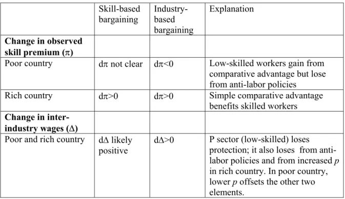
(19) The change in the premium is (9). dπ = dp( y, dt ) If Heckscher-Ohlin is right, dp<0 in poor countries, and since labor reforms do. not affect the observed premium, we must also have dπ<0. The opposite holds for the rich countries (dπ>0). Note that the change in the observed premium will not depend on what happens to labor market conditions (that is, on labor market reforms) since these reforms have industry-wide effects and thus affect both skilled and unskilled workers equally. In other words, a change in s does not affect dπ. The inter-industry wage differential will be (10). ∆=. P = (1 + λt )(1 + s ) U. with the change (11). d∆ = λ (1 + s )dt + (1 + λt )ds < 0 Inter-industry wage differences will be reduced very strongly if protection from. external competition is associated with strong unionization (both dt<0 and ds<0). Liberalization erodes both of these advantages (enjoyed by assumption by the same sector). To sum up. In a model with the same skill composition across sectors, if bargaining is skill-based, the skill premium would most likely go up in both poor and rich countries. If bargaining is industry-wide, then the skill premium will rise in income level. As for inter-industry wage differences, they will go down regardless of the type of bargaining and income level of the country. The decrease however will be greater if protection from external competition goes together with strong unionization. Since these. 19.

(20) two elements are likely to be found together more often in rich countries, inter-industry wage differences will be reduced more there.16 Introducing different skill-intensities. So far we have assumed that the skill intensity of the two industries is the same: each had the same share of skilled and unskilled workers. This is clearly an unrealistic although helpful assumption. By removing it, we may affect the conclusions regarding the effects on inter-industry inequality. 17 We shall consider first the case of skill-level bargaining. The ratio between the average wages will be ∆=. (12). P σ 1wup + (1 − σ 1)wsp σ 1w(1 + λt )(1 + s ) + (1 − σ 1)w(1 + p)(1 + λt ) = = = U σ 2 wuu + (1 − σ 2)wsu σ 2 w(1 + s) + (1 − σ 2)w(1 + p) ∆ = (1 + λt ). σ 1[( s − p)] + (1 + p) σ 2[( s − p)] + (1 + p). where σ1=low-skill labor intensity in the protected sector, and σ2=low-skill labor intensity in the unprotected sector. Note that if the shares are the same, the second term in (12) becomes unity. In accordance with empirical studies reviewed above (Richardson 2000, Harrison and Hanson 1999; Currie and Harrison 1997; and also Winters, McCulloch and McKay 2004, p. 100) we assume that prior to trade reforms protection is biased toward the low-skilled sector in both poor and rich countries. Consider now the polar case where σ1=1 and 16. Since labor compositions are the same across sectors, the sources of inter-industry wage differences are either (or both) tariffs or unionization premium. If bargaining is skill-based, then liberalization will erode the unionization premium, and ∆ must go down. If bargaining is industry-based, then liberalization will erode protection rents and unionization premium, and ∆ must again go down. The only other possibility— which we explicitly exclude here—is a combination of protection for one sector and collective bargaining for the other. In that case, change in ∆ would be ambiguous.. 17. Inter-occupational inequality will not be affected by different sectorial skill intensity. It is simply the ratio between ws and wu and that does not depend on what is the percentage of skilled and unskilled workers in different sectors.. 20.

(21) σ2=0, viz. protected sector is entirely low skilled while unprotected sector is entirely high-skilled. In addition, since protected sector is high-skill intensive, it is logical that its average wage is greater, and hence that U/P ratio represents now an indicator of inequality. For this to hold the effect of higher skill intensity must overwhelm the effect of protection. The expression (12) then becomes ∆=. U 1 (1 + p) = P (1 + λt ) (1 + s ). Accordingly, the change in inter-industry inequality will be. (13) d∆ =. − λ 1+ p (1 + p) 1 dt + dp − ds 2 (1 + λt )(1 + s ) (1 + λt ) 1 + s (1 + λt )(1 + s ) 2. where we take into account as before that dt<0, ds<0 and dp>0 (for the rich country) and dp<0 (for the poor country). Expression (13) will be definitely positive for the rich country. This can be relatively simply explained. Consider a rich country like the European Union or the United States that protects its low-skill intensive industries (say, textiles or steel). The tariffs “artificially” raise the average wage of the protected sector. In addition, that sector, being predominantly low-skilled, is more unionized and enjoys a “union rent” as well. The wage differential between it and the unprotected sector will be small. In other words, steel workers’ wages compared to those in unprotected sectors will be high. Trade liberalization by destroying the premium enjoyed by the protected sector and by reducing the “union rent”, will lower the relative wage of steel workers and the wage gap between the two sectors will increase.18 Moreover, the pure skill premium—which favors skilled workers in rich countries—will also move against the protected sector. Thus, liberalization will hurt the protected sector on all three accounts.. 18. Note however that if the pre-reform average wage of the protected sector is less than of the unprotected sector, then the opposite follows. In other words, in our model the P/U ratio plays the role of an inequality measure which it can only so long as P>U.. 21.

(22) For the poor country, expression (13) cannot be signed unambiguously, because the declining premium will work in the opposite direction from t and s. While the latter two will, as in the rich country, negatively affect the wage in the (low-skilled) protected sector, a decline in the premium may on the other hand fully or partially offset this loss. When bargaining is industry-based and skill compositions differ between the industries, ∆=P/U becomes. ∆=. p +1−σ 2 p U 1 = P (1 + λt )(1 + s ) p + 1 − σ 1 p. which in the polar case of σ1=1 and σ2=0 becomes ∆=. 1+ p (1 + λt )(1 + s ). Now the change in inter-industry inequality will be (14). d∆ =. (1 + p ) 1 − λ (1 + p) dt − ds + dp 2 2 (1 + s )(1 + λt ) (1 + λt ) (1 + s ) (1 + λt )(1 + s ). We deal with the same situation as before. All three relevant factors (dt, ds and dp) will contribute to make expression (14) positive for rich countries, while dp>0 will provide an offsetting element in the case of a poor country. Summary. It is now time to summarize the key implications of our model. Consider first the change in the observed skill premium (π). It does not depend on skill composition across sectors, so our earlier conclusions derived for the case of equal skill composition across sectors will hold. There we found that with skill-based bargaining, dπ is likely to be positive for both poor and rich countries; with industry-wide bargaining, we can expect the skill premium to rise (in response to liberalization) as country’s income increases.. 22.

(23) Let us move now to the change in inter-industry inequality (∆). There skill composition between sectors does matter and we shall therefore look at these conclusions only. There we found that d∆ will be unambiguously positive for rich countries while the sign for the poor countries depended on the relative strength of the skill premium versus the two rents effects. While these conclusions are relatively straightforward, they have been obtained at the cost of several strong assumptions that need to be re-listed explicitly. They are, first, that, after liberalization, the skill premium (p) increases with average income of the country. This derives from the simplest formulation of the theory of comparative advantage. Notice however that we introduce a distinction between a “pure” skill premium p, and the observed skill premium π which allows us to take a more nuanced view. Second, we assume that the unionization rent is captured by the same sector that is being protected. This is based on the empirical observations from the rich countries and a political economy view which holds that a sector which is strong enough to “exact” protection will be strong enough to bargain domestically as well. Moreover, ability to organize in order to bargain domestically may be the prerequisite to be strong enough to bargain for protection from foreign competition as well. In that case, the two rents have to go together. Third, we have, following a recent number of empirical studies, assumed that low-skilled sector is protected not only in rich countries but also in poor countries. Combining assumptions 2 and 3, it can be quickly seen that low-skill intensity, protection from external competition and ability to bargain domestically will go together in both poor and rich countries. Obviously, in further work some of these assumptions could be relaxed. Finally, a fourth, rather technical assumption, is needed to generate our results. It is that the average wage in the unprotected sector is greater than the protected sector’s average wage, so that U/P>1 serves as an indicator of inequality. Now, since in both poor and rich countries the protected sector was assumed to be low-skilled, that assumption seems reasonable.. 23.

(24) The changes in inter-industry differences following trade liberalization are summarized as in Table 1. Table 1. Change in various types of wage inequality in conditions of trade and labor liberalization Skill-based bargaining. Industrybased bargaining. Explanation. Change in observed skill premium (π) Poor country. dπ not clear. dπ<0. Rich country. dπ>0. dπ>0. Low-skilled workers gain from comparative advantage but lose from anti-labor policies Simple comparative advantage benefits skilled workers. d∆ likely positive. d∆>0. Change in interindustry wages (∆) Poor and rich country. P sector (low-skilled) loses protection; it also loses from antilabor policies and from increased p in rich country. In poor country, lower p offsets the other two elements.. Can we observe skill premium increasing in both countries? For rich countries, the answer is easy: whether bargaining is skill- or sector-based, skill premium should go up as trade is liberalized. But for a poor country, observed skill premium will go up only if bargaining is skill-based and the effect of dismantling pro-labor regulations overwhelms the “pure” trade effect that is in principle favorable to unskilled labor. 19. 19. A further modification of this static model—moving it toward a general equilibrium type of models— could include the effects of wage changes brought about by reform on labor demand and supply. These are longer-term effects and we do not take them into account here. For example, after the reform in a rich country, there should be an increased demand for skilled workers in the unprotected sector. This should bring about an increase in their numbers, and the U sector will become (even) more skill-intensive compared to the P sector. The effect on the measured ∆ will be to reduce it even further as the average wage in unprotected sector catches up with the average wage in protected sector. (As mentioned before, we assume that in the short-run at least, there is no “overturn” of this relationship, so that P/U ratio does not become less than 1. However, in the medium term as U sector becomes more skill-intensive and P sector loses its skilled workers, this could be the case. ). 24.

(25) 4. Data description Inequality measures. The first of the two large databases we use to derive inequality measures is that of Occupational Wages around the World (OWW). As mentioned before, the data cover the period from 1983 to 1999 and more than 150 countries. The coverage in all its dimensions, however, is problematic and fragmentary. Although there are 156 countries in total, each country does not provide data (occupational wages) for every year. The yearly country coverage varies between 48 and 76. Occupations included also vary from country to country. Moreover for a given country even when it does provide the annual data, the occupational coverage is not necessarily uniform for each year. 20 Furthermore, it should be noticed that each observation is an observation on “habitual” country-wide wages for a given occupation. Thus some averaging is already built into the data. That however need not be a problem since, for example, the differences in earnings by skill levels are also based on averaging. There is however a difference in that the latter are obtained through a statistical analysis that covers a well defined spectrum of wage earners (labor force survey) and controls for other relevant factors (gender, experience), while the ILO data represent a mish-mash of average “habitual” wages for different underlying populations: some countries—for some years— report monthly wage rates, other report collectively bargained wages, yet others report hourly wages. At times men and women are combined, and at times only wages for men are reported. Freeman and Oostendorp overcome the problems of data comparability by “calibration” which is essentially a process of finding the adjustment coefficients (based on a regression analysis) for the data given in a “non-standard” form, where the standard form is defined as the most common form being used in the dataset, viz. monthly wages for male workers.21. 20. For example, the US gives the data on 11 occupations in 1983 and 150 occupations in 1999. They do several such calibration and show (in an Annex) that the results (inequality statistics) do not depend on a particular calibration. For our calculations, we have used their suggested base-wage calibration denoted x1wu in the oww.dta database.. 21. 25.

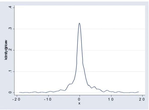
(26) The great advantage of the database (which incidentally also makes the calibration possible) is its size: in the Freedman-Oostendorp’s “summary” (compendium) of the ILO sources,22 there are more than 72,000 observations of average occupational wages. For each of the three indexes of inter-occupational wage inequality which we calculate (Gini coefficient, standard deviation and absolute mean deviation from the median), inequality indexes are calculated only for the country/years that contain more than 15 occupational wages (of the “calibrated” type). After this “filter” and a few others (dropping data for a number of small island economies and dependencies), we are left with 680 observations (country/years) covering the 1983-99 period and 118 countries. The average Gini is about 23.8, the median 21.7, with the standard deviation of about 10. A summary of the data is given in Annex 1 (Table 1). These inequality statistics can be, according to Freeman and Oostendorp, regarded as both indicators of occupational wage inequality and skill premium.23 Figure 1 shows the distribution of annual changes in the calculated Gini coefficients (dginioww) over the 1984-1999 period. As we observe, the distribution is close to being symmetrical and normal, with the mean which is slightly positive (0.17 Gini point) and a zero median.. 22. The Freeman-Oostendorp database is indeed a “summary” of ILO data since the data on occupational wages have been collected by the ILO since 1924 while Freeman-Oostendorp data begin with 1983. 23 Implicitly, the greater the dispersion of inter-occupational wages, the greater the return to skills.. 26.

(27) Figure 1. Distribution of changes in occupational wage inequality (dginioww). 0. .1. kdensitydginioww .2. .3. .4. (in percentage points, 1983-1999). -2 0. -10. 0 x. 10. 20. Note: There are 532 dginioww observations. Changes are expressed in Gini points.. The second large database of inter-industrial wage differences is created by James Galbraith and associates and is known as the University of Texas Inequality Project (UTIP) database (see Galbraith and Kum, 2003).The original data come from UNIDO statistics. The UNIDO statistics provide average manufacturing pay by industry. The number of industries (which provide their mean wages) varies between countries and years. On average, there are 24 industries per country/year (with the standard deviation of about 7). From these average industrial wages for a given country/year, Galbraith and his associates calculate Theil index of inequality (variable theil). The UTIP database covers on average about 90 countries annually over the period 1975-99.24 In total, we use 24. The data are available at http://utip.gov.utexas.edu/. More recently, the database has expanded to the years prior to 1975. As of January 2004, UTIP data base has almost 3200 country/year Theils, and covers more than 150 countries.. 27.

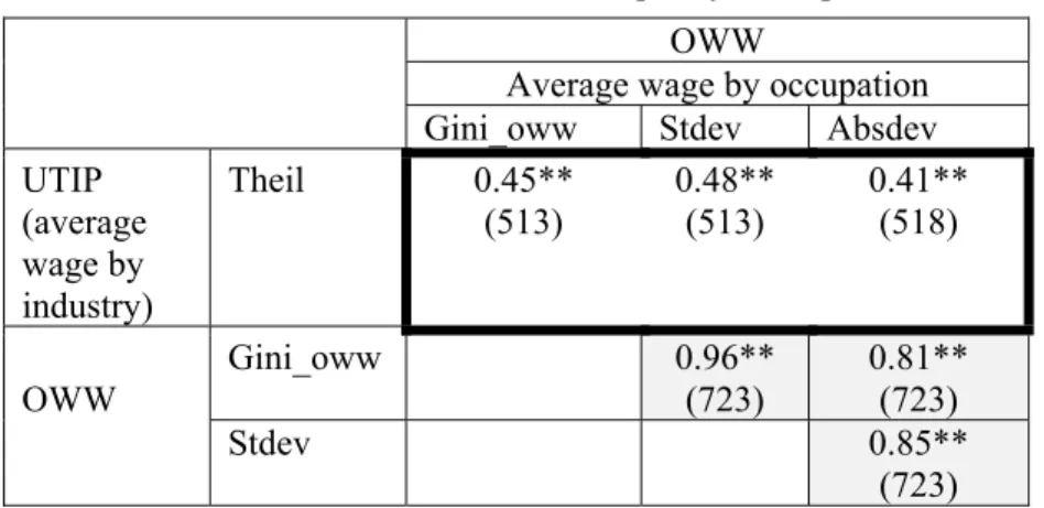
(28) 1651 Theil indexes from 141 countries (see Annex 1 Table 2 for details). The average Theil is 5.5, the median 3.8 and the standard deviation 6.4. In about ten percent of observations inter-sectoral wage differences are minimal with Theils less than 1. Many of these cases include developed countries (Nordic countries, the Netherlands) but also Algeria, Cuba, Iran, and until the mid-1980s China.25 Table 2 shows simple correlations between different inequality measures from the two databases. We have three inequality statistics from the OWW database (Gini coefficient, standard deviation and absolute mean deviation from the median) and only one from UTIP (Theil coefficient). Different inequality statistics from the OWW database are obviously strongly correlated (see the shaded cells). The correlation between Theil index from UTIP and Gini from the inter-occupation inequality is much less—around 0.4 (see also Figure 2). Still it shows that higher skill premium is associated with greater inter-sectoral inequality.. The correlation between the changes in the two measures. (which we shall be using in our regressions) is virtually zero however.. 25. It will be noticed that we do not use Gini coefficient here (although we would have linked, for a more direct comparison with OWW dataset to do so). The reason is that UTIP database does not provide individual mean industrial wages which would allow us to calculate different inequality measures. The authors only provide the “finished” statistic, that is the Theil index, and not the underlying data. This is not the case with the OWW database where individual occupational wages by country/year are available and one can thus calculate various inequality indexes.. 28.

(29) Table 2. Simple correlations between various inequality measures and inequality concepts. UTIP (average wage by industry). Theil. OWW Average wage by occupation Gini_oww Stdev Absdev 0.45** 0.48** 0.41** (513) (513) (518). Gini_oww. 0.96** (723). OWW Stdev. 0.81** (723) 0.85** (723). Note: Number of observations given between brackets. Each country/year represents one data point, that is for each country/year, there is one inequality statistic. The level of significance (null hypothesis: correlation = 0): ** = less than 1%, * = less than 5%. Shaded are cells with correlation coefficients calculated between various inequality measures from the same database.. 0. .2. gini of wages, x1wu .4 .6. .8. Figure 2. Inter-occupational (Gini) and inter-industry (Theil) inequality. 0. .1 .2 Galbraith: Theil of inter-ind. w ages. .3. Note: Calculated from 513 observations from 79 countries Total number of observations is 723 (from 103 countries) for inter-occupational inequality and 2160 (from 141 countries) for inter-industry inequality.. 29.

(30) Import liberalization and globalization measures. Trade liberalization can also be measured in many different ways. The primary choice is between policies – tariff reductions, elimination of non-tariff barriers, etc -- that are thought to help globalization, and outcomes such as trade volumes that are a consequence of trade policies. Both approaches have been used in the literature. Most of the studies reviewed here used trade shares as their measure of globalization. Lundberg and Squire (2003) use the Sachs-Warner Index which, although linked to policies, has been criticized on the grounds that it captures more that trade policy. Edwards (1997) uses a variety of policy measures: average tariff; average QR (quantitative restrictions) coverage; and average black-market premium.. Savvides. (1998) uses a specially created measure of protection covering both tariff and non-tariff barriers compiled from UNCTAD data at the four-digit level of the Customs Cooperation Council Nomenclature. The measure is only available, however, for 1988. Finally, those studying wage-inequality within a country are often able to make use of industry-specific tariff rates and quotas. All of the various ways of specifying variables representing trade liberalization are useful and answer interesting questions. If trade volumes are chosen then the study says something about the impact of trade volumes on inequality. And for some purposes that may be an interesting question. But, in our view, it does not say much about the impact of policy on inequality, primarily because trade volumes are not determined exclusively by policy. A wide range of factors will influence a country’s trade volume: country’s geography, technology, demand conditions in importing countries, competitors’ supply conditions, weather, and so on. Even attempts to control for these other factors will inevitably leave a residual that captures more than trade policies. We suspect that widespread reliance on trade volumes in the empirical literature reflects the relative ease of obtaining data compared with the difficulty of achieving the same for trade policies. Since we are interested primarily in how pro-openness reforms affect inequality, we prefer to focus on policies and thus place ourselves squarely in the policymaker’s corner. We attempt to answer the question that many policy-makers naturally 30.

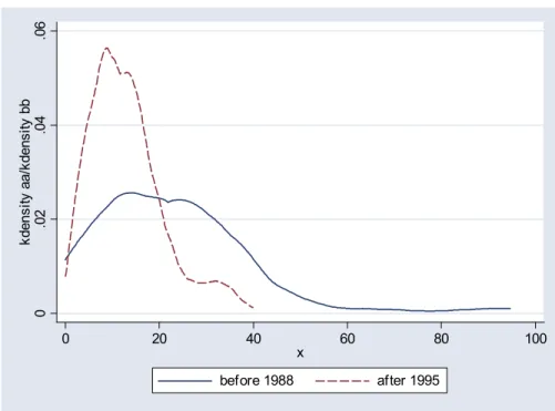
(31) formulate when they envisage trade reforms: “What will be the effect of liberalization reforms such as tariff reduction on wage differences between various occupations and industries?” For import liberalization, we use the World Bank measure of unweighted average tariff (variable tarf) rate which covers the period from 1980 to 2000, includes 144 countries, and provides 1255 observations (county/years) in total. The list of countries and number of country/years are shown in Annex 1 (Table 3). Over this period, the average tariff rate (calculated across the available countries) has been reduced from 28 percent to about 10 percent. Figure 3 how the distribution of average tariff rates by countries has shifted leftward with the median, mean, and the standard deviation all significantly less today than in the early and mid-1980’s.. 0. kdensity aa/kdensity bb .02 .04. .06. Figure 3. Distribution of countries’ average tariff rates in the periods 1980-88 and 1995-2000. 0. 20. 40 before 1988. x. 60. 80. 100. after 1995. Note: average tariff rate for a country over a period (1980-88 or 1995-2000) represents one observation. Number of countries is 106 for the first and 132 for the second period.. The reduction has affected both rich and poor countries. The average tariff rate in poor countries (defined as those with GDP per capita less than $9000 at international. 31.

(32) prices) was reduced from 33 percent to 13 percent; for the rich countries, the reduction was from 16 to 7 percent. The pattern of reduction for both poor and rich countries has been very similar to the one shown in Figure 3: not only are average tariff rates less in 2000 than some twenty years ago, but the differences between the countries is much smaller too (in other words, the distribution of average tariff rates across countries is much more compressed now than in 1980). To account for the possibility mentioned above that individual countries are “globalized” not directly through their own policies but through the effect that policies of their trading partners have on themselves, we create a special globalization variable. It is calculated as follows. For each country, we take its three largest importers and calculate their import shares (for the United States, for example, they would be Canada, China and Mexico). These import shares are then multiplied with a variable denoting presence or absence of trade reform in the three countries.26 The result gives an import-weighted indicator of presence of trade reforms in country’s most important trading partners. Presumably, if a country’s key trading partners are engaged in reforms, this puts pressure on the country in question to reform as well. One problem when trying to link tariff liberalization reforms to domestic outcomes such as wage distribution is that they are seldom undertaken in isolation. Most frequently, pro-openness trade reforms are accompanied by other “globalization” policies that may well affect labor market outcomes: for example, easier direct or portfolio investment by foreign residents or more liberal regulation of international labor flows. And just as frequently trade reforms are accompanied by domestic reforms that impact directly on labor markets: “flexibilization” of the labor market, changes in the minimum. 26. This is a three-way variable: there could be a pro-openness reform, anti-openness reform, or no change. The calculation is based on Free the World (FTW) measure of trade taxes: if they decrease sufficiently, a country is deemed a reformed over the entire five-year period (FTW data are available at five-year itervals). “Sufficiently” is defined as reduction in trade taxes/trade ratio by more than ½ of the world standard deviation in that variable. In other words, if world’s standard deviation of trade taxes/trade variable is 5 percent, than if country’s trade taxes/trade ratio goes down by 5 percentage points, it is deemed a proopenness reformer. The opposite is the case for anti-openness reforms. Free the World data are available at www.freetheworld.com. The report is issued by the Fraser Institute, Vancouver (see http://www.fraserinstitute.ca/shared/readmore.asp?sNav=nr&id=537).. 32.

(33) wage legislation, more (or less) liberal severance pay, reform in the pension regimes etc. These accompanying domestic reforms often concern labor—whether they are “anti” or “pro” labor. Sometimes “anti” labor legislation accompanies openness reforms because it is felt that liberalization in the foreign arena can be emptied of content (or cannot produced the desired results) if there is no improvement in the domestic legislation, i.e. if the latter is deemed too restrictive. Mexico provides one such example (Robertson, 2000 and Hanson and Harrison, 1999). Alternatively, labor policies can, for a segment of labor force at least, become more generous if that is the short-term cost the government needs to pay in order to convince trade unions not to wreck the reforms. In that case, more generous severance pay, low interest loans to start own businesses, early retirement schemes can all be used to reduce the resistance to reforms and to “buy off” potential losers. In addition to labor reforms, there may be also “accompanying” financial reforms: liberalization of interest rates, increased competition in the banking sector etc. All of this complicates any attempt to isolate the impact of trade reform on wage inequality. We shall therefore try to control for some of these other policies (labor markets, social transfers). To measure labor market conditions, we use Labor Market Data Base constructed by Martin Rama and Rachel Artecona (see Rama and Artecona, 2002). 27 Their database has, at five-year intervals (year 1975, 1980 etc.) a number of labor-related measures such as social security contributions (in percentage of gross salary), unemployment rate, replacement rate in case of unemployment etc. For our purposes, that is bearing in mind the model described above, two variables are of particular interest: share of labor force covered by collective agreements, and share of the unionized labor force. They do not allow us to distinguish between the type of unionization (skill- or industry-based) which we considered in our model, but they do allow us to proxy the power of trade unions and organized labor.. 27. The data have been kindly supplied by Martin Rama.. 33.

(34) 5. Level of protection and occupational wage inequality. We look first at the level relationship between occupational wage inequality and mean tariff rate.. Figure 4 shows that occupational wage inequality (or returns to. education) tend to decrease with average income level of the country (panel a). This is of course what we expect since rich countries have greater proportion of skilled labor. Likewise average tariff rate tends to be lower in richer countries (see panel b). Finally, returns to education increase in level of protection (panel c). This last point would seem to imply that protection is calibrated in such a way as to boost incomes of more skilled workers.28 However, this relationship may be only apparent and due to the fact that that poorer countries tend to have, as we have just seen, higher average tariff rate. In effect, once we control for the difference in the returns to education that is due to income levels, the correlation between returns to education and protection vanishes (panel d). It is no longer statistically significant. We can conclude that in a cross-sectional setting, average level of protection and occupational wage inequality do not display any obvious relationship—once we adjust for the fact that poorer countries tend to have both higher returns to education and higher levels of protection.. 28. Which, by the way, would contradict the general finding of higher protection for less-skilled industries (see discussion above).. 34.

(35) Figure 4. Occupational wage inequality, average level of protection and mean income (b) Average tariff rate and level of income. 0. 0. gini of wages, x1wu/Fittedvalues .2 .4 .6. .8. unweightedaveragetariff ratefromWBsources/Fittedvalues 20 40 60 80 100. (a) Occupational wage inequality and level of income. 6. 7. 8 9 lo g (g d p p p ). 10. 11. 6. g in i o f wa g e s , x1 wu F itte d v a lu e s. 8 9 lo g (g d p p p ). 10. 11. u n we ig h te d a ve ra g e ta riff ra te fro m W F Bitte so du rce va lu s es. (d) Occupational wage inequality (controlled for income) and average tariff rate. 0. -.2. -.1. res/Fittedvalues 0 .1. gini of wages, x1wu/Fittedvalues .2 .4 .6. .2. .3. .8. (c ) Occupational wage inequality and average tariff rate. 7. 0 20 40 60 80 100 unweighted average tariff rate from WB sources. 0 20 40 60 80 100 u n we ig hte d a ve ra g e ta riff ra te fro m W B so u rce s. gini of wages, x1wu Fitted values. re s. 35. F itte d va lu es.

(36) But this does not necessarily imply that there is no relationship between the changes in mean tariff rate and changes in returns to education.. The correlation. coefficient is –0.10 (see Figure 5) and is significant at the 10 percent level. It suggests that there may be a weak negative (and uncontrolled for other variables) relationship such that a decrease in domestic protection (i.e., liberalization) is associated with an increase in returns to education. 29. -20. -10. dginioww/Fittedvalues 0. 10. 20. Figure 5. Relationship between change in mean tariff (dtariff) and change in occupation wage inequality (dginioww). -3 0. -2 0 -1 0 0 10 c h a n g e in W B m e a n t a r if f r a t e d g in io w w. 20. F it t e d v a lu e s. Note: The regression coefficient remains negative and significant if outliers, that is observations such that dtarf<-25 are eliminated.. 29. The two variables are run here and further below contemporaneously. However since the data on mean tariff rates are often not available for all consecutive years, dtarf variable is defined in such a way as to include annual changes wherever available, that is, not only tarf (t) – tarf (t-1) but also tarf(t) – tarf(t-2) when tarf(t-1) is not available. Thus dtarf is partly lagged (about 20 percent of observations refer to changes between years t and t-2).. 36.

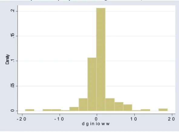
(37) Figure 6 shows the distribution of changes in occupational Ginis for county/years for which we have corresponding data on changes in protection (that is, Figure 6 shows the distribution of dginioww for our sample, not for all the observations of dginioww that we have30). There is, on average, a tendency for occupational inequality to increase (the mean Gini change is +0.36, median +0.05) matching the tendency of tariff rates to go down over the last twenty years (in our sample, the average tariff change is –1.05 percentage points, the median –0.2). Thus there is some prima facie evidence that decreases in protection and increases in occupational wage inequality may be related.. 0. .05. Density .1. .15. .2. Figure 6. Distribution of changes in occupation inequality (when both data on occupational inequality and tariff changes are available). -2 0. -1 0. 0 d g in io w w. 10. 20. We look further at this relationship by breaking down changes in returns to education (dginioww) across average protection changes (Table 3). There is some evidence that deeper cuts in protection are associated with greater increases in 30. The shape of the two distributions though is almost exactly the same. The number of cases, however, is quite different. Our sample contains only 268 observations while there is a total of 532 observatioons of changes in occupational inequality.. 37.

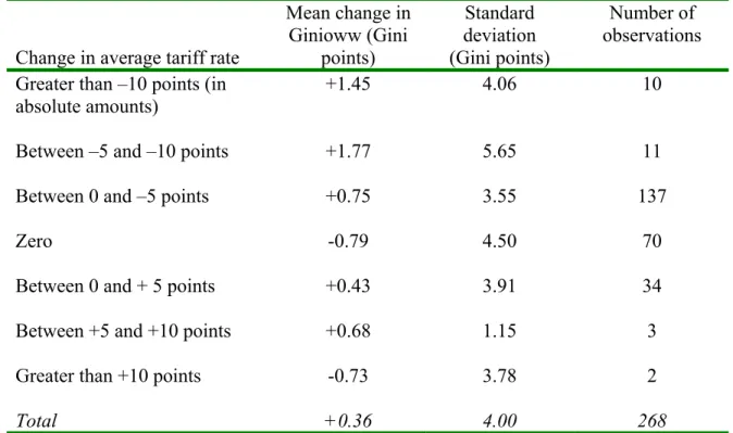
(38) occupational inequality. For example, when tariff protection goes down by more than 10 percentage points, occupational Gini increases on average by 1.45 points. When the reduction in protection is less (between 0 and 5 percentage points), the increase in wage inequality is also smaller (+0.75 Gini points). This relationship is not very strong and uniform though. Change in Gini is, on average, positive even when average tariff rate goes up (by less than 10 percentage points). This in turn suggests that other factors must be at play too. Furthermore, in a number of cases where there was no change in mean tariff rate, average (and median) wage inequality tended to go down. On balance, we conclude that while there is some evidence that import liberalization is associated with increasing occupational wage inequality this is unlikely to be the only factor that matters. Table 3. Relationship between occupational wage inequality and protection (average tariff rate) Mean change in Ginioww (Gini points) +1.45. Standard deviation (Gini points) 4.06. Number of observations. Between –5 and –10 points. +1.77. 5.65. 11. Between 0 and –5 points. +0.75. 3.55. 137. Zero. -0.79. 4.50. 70. Between 0 and + 5 points. +0.43. 3.91. 34. Between +5 and +10 points. +0.68. 1.15. 3. Greater than +10 points. -0.73. 3.78. 2. Total. +0.36. 4.00. 268. Change in average tariff rate Greater than –10 points (in absolute amounts). 10. We next split the sample into rich and poor countries (Table 4). We take $PPP 9,000 (at 1995 prices) as the cut-off point. This means that in 1980 about three-quarters of all countries in the world are regarded as poor (the proportion is about 70 percent in. 38.

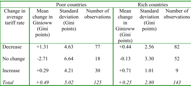
(39) 2000.) Since the data for the rich countries are, on average, more frequently available than for the poor, the cut-off off point neatly splits our sample into about two halves. Table 4. Relationship between inter-occupational wage inequality and level of protection (average tariff rate) in poor and rich countries. Change in average tariff rate. Decrease. Poor countries Rich countries Standard Number of Number of Mean Standard Mean change in deviation observations change deviation observations (Gini in (Gini Ginioww Ginioww points) points) (Gini (Gini points) points) +1.31 4.63 77 +0.44 2.56 82. No change. -2.71. 6.64. 18. -0.13. 3.30. 52. Increase. +0.29. 4.21. 30. +0.71. 1.01. 9. Total. +0.49. 5.02. 125. +0.25. 2.80. 143. Note: poor countries are defined as those with GDP per capita less than $9000 at international 1995 prices. Rich, those above that threshold.. The table illustrates that the same regularity applies to both poor and rich countries: decreases in protection are associated with higher wage inequality, but so are (although the magnitudes are substantially lower) increases in protection. It is mostly when there is no change in mean tariff rate that we find shrinking occupational wage distribution. In effect, out of 122 cases when occupational inequality goes down, about one third (39) involve situations with no change in mean tariff rate. Poor countries display in all cases (decrease, no change, or increase in protection) greater variability in outcomes. This is illustrated in Figure 7 where we look at changes in occupational Gini when protection is reduced. The strongly spiked density function for the rich countries (dashed line) shows that reduced protection is accompanied by relatively small and very similar changes in rich countries’ Ginis; in contrast, in poor countries, Gini changes (solid line) are much more spread out. The hypothesis of equality of the two distributions is soundly rejected (the Kolmogorov-Smirnov test is significant at less than 0.1 percent).. 39.

No results found