S
TRUCTURAL EFFECTS OF A
SUSTAINED RISE IN THE TERMS OF
TRADE
Adam McKissack, Jennifer Chang, Robert Ewing and Jyoti Rahman
Treasury Working Paper
2008 — 01
July 2008
An earlier draft of this paper was presented to the Treasury Academic
Consultative Committee Workshop on Terms of Trade held on
14 February 2008. The authors are from Domestic Economy Division (DED),
the Australian Treasury. The authors would like to thank Jyothi Gali for
performing the CGE simulation in this paper. The paper also benefited from
comments provided by Jason Allford, Jeff Borland, David Gruen,
Tony McDonald, Paul O’Mara, Niloofar Rafiei, David Stephan, and colleagues from DED. The views expressed in this paper are those of the authors and not
A
BSTRACT
While previous terms of trade booms have tended to be short‐lived, there are
reasons to believe that the current boom could be more enduring. This paper
considers the implications for the Australian economy in the event that recent
rises in the terms of trade are sustained, with a focus on labour market, industry and regional implications.
Thus far, the economy’s reactions to the terms of trade boom have largely
matched the predictions of economic theory: incomes have risen, as have
employment and investment, in particular for the mining industry and regions
where mining is concentrated. However, we have not seen so‐called
‘Dutch disease’ effects associated with a higher exchange rate flowing through
as strongly as could be expected in the manufacturing industry and other traded parts of the economy.
Adjustments to the boom have thus far taken place in a position of less than full
employment, so the resources sector has to date been able to utilise previously
unemployed factors of production rather than simply attract factors from other
sectors of the economy. Going forward, expanding labour supply in the
resource‐rich regions of the country will be a central policy challenge.
If well managed, the transition to a higher terms of trade presents an
opportunity to raise Australian living standards. But the challenges in ensuring
a successful transition are significant and will test our policy frameworks in
ways they have not been tested before.
JEL Classification Numbers: F16, F22, F47, J61.
C
ONTENTS
1. INTRODUCTION...1
2. THE CURRENT TERMS OF TRADE BOOM...2
3. THE ECONOMICS OF A TERMS OF TRADE BOOM...5
4. EFFECTS OF A HIGH TERMS OF TRADE — EVIDENCE...8
5. WHAT IF THE TERMS OF TRADE RISE IS SUSTAINED?...17
5.1 State labour markets and labour mobility...22
6. POLICY IMPLICATIONS AND CONCLUSION...30
7. BIBLIOGRAPHY...34
APPENDIX A MODEL DESCRIPTION...36
1. I
NTRODUCTIONSwings in Australia’s terms of trade have been a key channel for the
transmission of shocks from the rest of the world to the domestic economy
throughout our economic history as a small, open, commodity‐exporting
economy. However, the recent sharp upswing in the terms of trade represents
the largest movement in the terms of trade since the 1950s peak associated with the Korean War‐induced wool price boom (Chart 1).
Chart 1: Terms of Trade
40 60 80 100 120 140 160 1900-01 1918-19 1936-37 1954-55 1972-73 1990-91 2008-09 40 60 80 100 120 140 160 Forecasts Index (2005-06 = 100) Index (2005-06 = 100)
Source: Commonwealth of Australia (2008).
The terms of trade swings of the past were generally associated with periods of
economic instability. Following the mid‐1980s terms of trade decline, economic
reforms were made to diversify and modernise the Australian economy to
improve its capacity to deal with shocks from the world economy. A relative
period of stability in the terms of trade through the 1990s created a sense that the volatility in the terms of trade may have been a feature of the past. However, the recent boom associated with the rise of China and India has brought the terms of trade back into the central frame for economic policy makers.
This paper examines recent movements in the terms of trade and discusses their
implications for the Australian economy. While previous booms have tended to
be short‐lived, there are reasons to believe that the current boom could be more
enduring. In other words, the upswing in the terms of trade of recent years could
have a large structural component, rather than being purely cyclical. The paper
considers the implications for the Australian economy in the event that recent
rises in the terms of trade are sustained, with a focus on labour market, industry
and regional implications. The paper concludes with a discussion of policy
implications.
2. T
HE CURRENT TERMS OF TRADE BOOMFollowing a peak in the terms of trade in the mid‐1970s which was driven by a
rise in agricultural commodity prices, the terms of trade trended downwards,
reaching a trough in the mid‐1980s around the time the former Treasurer,
Paul Keating, made his famous ‘banana republic’ remarks.1 Following this
period, the terms of trade experienced a period of relative stability.
This relative stability in the terms of trade followed a period of reform which
opened the Australian economy to greater competition from abroad and
enhanced the flexibility of the economy to respond to shocks. These reforms
included liberalisation of Australia’s foreign exchange, trade and investment
regimes, financial markets deregulation, and labour and product market
reforms.
During this period, Australia’s exports and imports became more diversified. Australia’s exports, for example, became less dependent on commodity exports,
although commodities remained the largest component. Commodities
comprised around 65 per cent of Australian exports in the mid‐1970s compared
with around 57 per cent in 2007 (Chart 2). The fall in the share of commodities largely reflects the declining importance of rural commodities. The share of rural commodities fell from around 35 per cent in the mid‐1970s to around 11 per cent in 2007.
Chart 2: Share of total export values, 1974-75 to 2006-07
0 20 40 60 80 100 1974-75 1982-83 1990-91 1998-99 2006-07 0 20 40 60 80 100 Rural commodities Non-rural commodities ETMs Other goods Services
Note: ETMs — ‘Elaborately Transformed Manufactures’. Source: ABS Balance of Payments, Catalogue Number 5302.0.
A more stable terms of trade during the late‐1980s and the 1990s led credible
commentators to consider the volatility in the terms of trade to be more a feature of history. In the 2002‐03 Budget papers Treasury noted that:
‘The terms of trade is likely to be more stable in the future because of the
diversification of Australia’s trade baskets (across products and destinations),
events, and the generally more stable global economy’ (Commonwealth of Australia 2002).
While soundly based, the above comment proved not to be one of Treasury’s
better predictions, with the terms of trade subsequently rising to their highest level in over 50 years. What was under‐estimated at the time (by most informed
observers, including the mining companies themselves) was the impact on
commodity prices of the rise of China and other emerging economies.2
Import prices have made some contribution to the higher terms of trade over the past two decades.3 But the more recent upswing in the terms of trade reflects
increased demand from China and other emerging economies for Australia’s
non‐rural commodity exports (Chart 3).
Chart 3: Export and Import prices — SDR
80 100 120 140 160 180
Mar-80 Mar-84 Mar-88 Mar-92 Mar-96 Mar-00 Mar-04 Mar-08 80 100 120 140 160 180 Exports Imports
Index (Dec 2001=100) Index (Dec 2001=100)
Note: SDR — Special Drawing Right.
Source: ABS Balance of Payments, Catalogue Number 5302.0.
2 For an analysis by Treasury on the implications of the rising economic importance of
China and India, see Commonwealth of Australia (2006).
3 In particular, prices of information and communications technology goods (comprising
automatic data processing (ADP) equipment, telecommunications equipment and parts
Since the March quarter 2004, export prices (in Australian dollar terms) for non‐rural commodities have increased by around 91 per cent, while total export
prices have increased by around 41 per cent. The aggregate increase has been
dominated by large rises in the prices of bulk commodities and base metals. For example, in this period, the prices for iron ore, metallurgical coal and thermal coal rose by around 165 per cent, 88 per cent and 86 per cent respectively. Export prices for metals also increased significantly, rising by around 60 per cent.
A rising terms of trade, be it from rising export prices or falling import prices,
generates increased purchasing power and higher incomes for the economy.
However, the short‐term effects of different drivers of the terms of trade will vary. Falling (Australian dollar) import prices will have broader direct effects on
the economy at the outset. Producers and consumers will benefit from cheaper
inputs and cheaper final goods as import prices fall. Rising export prices,
however, especially in the current environment of rising commodity prices, will
impact on particular industries initially before the benefits disseminate into the
wider economy. The more the exchange rate appreciates in response to higher
world commodity prices, the more the transmission will occur through lower
import prices (in Australian dollar terms) than otherwise.
The implications of the recent rise in the terms of trade for the economy more broadly are discussed in the next section.
3. T
HE ECONOMICS OF A TERMS OF TRADE BOOMWhat do higher terms of trade mean for Australia? This section reviews some
well‐known theoretical frameworks for thinking about the effects of a rise in the terms of trade. The section begins by examining simple, two‐sector comparative
static results, then extends the analysis to incorporate a third, non‐traded sector. Some dynamic considerations are then discussed to better understand real world adjustment processes.
The Heckscher‐Ohlin two‐sector model of international trade predicts patterns of
production and trade based on a country’s factor endowments. The model’s
central prediction is that countries will export goods that utilise the factors of production they are abundant in, and import goods whose production process is more intensive in the country’s scarce factors. So, for example, the model would
predict that Australia would export goods which are relatively intensive in
capital (commodities) and import labour‐intensive goods, such as
manufacturing.
Henry (2006) considers in some detail the situation where commodity prices rise
within the Heckscher‐Ohlin framework in an economy with two sectors —
mining and manufacturing. Commodity output rises as returns to that sector rise
and output in manufacturing falls. The mining sector draws capital and labour
from the manufacturing sector. The profit share rises on the basis that the
booming mining sector uses capital relatively intensely. Real income rises and
consumers are better off.
Various ‘Dutch disease’ models, such as those outlined by Corden (1984),
Corden and Neary (1982) and Gregory (1976), allow us to examine the
interaction between three sectors: the non‐tradable sector (such as retail trade), the booming tradable sector (commodities in the current Australian context), and
the lagging tradable sector (manufacturing, for example). A rise in the terms of
The resource movement effect refers to the rise in the demand for labour and
capital in the commodities sector leading to a shift in factors of production
toward this sector and away from the lagging manufacturing sector and
(initially) the non‐tradable sector. The spending effect occurs as a result of the extra income generated by the commodities boom. This increases the demand for
non‐tradable services, which in turn raises the demand for labour in the
non‐tradable service sector, attracting labour away from the manufacturing
sector.
As a result of the increased demand for non‐tradables, their price increases
relative to the price of traded goods (that is, an appreciation of the real exchange rate).
Considering dynamic effects, real income in the economy is unequivocally
higher than it was before, and consumers are better off in the long run. But what is the adjustment path?
Higher income leads to stronger domestic demand, which in turn raises demand for labour. If the economy is below full employment, stronger demand for labour
is likely to increase employment. Nearer to full employment, the increased
labour demand will largely be reflected in wage and price pressures because
increases in aggregate supply will lag increases in aggregate demand. How the
macroeconomy adjusts to the resultant inflationary pressure then depends on the
macroeconomic institutional arrangements in the country (see Gruen, 2006). In
the presence of an inflation targeting monetary policy framework and a floating
exchange rate, the adjustment involves some combination of a higher nominal
(and hence real) exchange rate and higher real interest rates. The higher
higher real interest rate also has a dampening effect on the non‐traded sectors of the economy, such as the retail and dwelling sectors.
In Australia, there is a geographical dimension to the rising terms of trade —
some States are much more intensive in the mineral resources that have
experienced large price gains.4 While the whole economy benefits from the rise
in the terms of trade, the resource‐rich States are likely to grow more strongly than others after the rise in the terms of trade. To the extent that there are rigidities in factor mobility between States, particularly for labour, this will slow
the adjustment process needed to facilitate stronger growth in the resource‐rich
States.
4. E
FFECTS OF A HIGH TERMS OF TRADE—
EVIDENCEThis section tests a number of propositions implied by the previous section
against the economic data both at the national aggregate level and the industry
and state levels. Industry comparisons focus in particular on the mining,
manufacturing and retail industries, which represent the booming traded sector,
the lagging traded sector and the non‐tradable sector. Construction is also of
interest, as an industry that has benefited directly from the mining boom. This
allows the industry effects associated with the Dutch disease models discussed
in the previous section to be tested against the data.
It is important, however, to keep in mind that rises in the terms of trade have not
been the only influence on the economy in recent times. Other significant
adjustment from a period of rising house prices, particularly in
New South Wales. Record high oil prices and the impact of a severe drought
have also been significant influences.
Proposition 1: income will rise but will rise more in the mining industry.
Higher commodity prices have caused incomes to grow across the economy and, as expected, incomes have increased more rapidly in the mining industry. In the three years since 2003‐04, mining’s share of total factor income has risen sharply (Chart 4).
Chart 4: Selected industries’ share of total factor income
4 6 8 10 12 14 16 1990-91 1992-93 1994-95 1996-97 1998-99 2000-01 2002-03 2004-05 2006-07 4 6 8 10 12 14 16
Mining Construction Manufacturing Retail trade
Per cent Per cent
Source: ABS Annual National Accounts, Catalogue Number 5204.0.
Mining profits have risen faster than profits in other industries in this period.
While profits have continued to grow across the economy, profits in other
industries have grown on average at a slower pace in the past three years than
over the previous decade.
This is illustrated in Chart 5 which shows average annual growth in the previous decade on the vertical axis and average growth in the past three years on the horizontal axis. The chart is divided by a 45 degree line, with any industry to the
right of this line experiencing higher average profits growth since 2003‐04 than
over the previous decade.
Chart 5: Growth in company gross operating profits by industry
0 10 20 30 40 0 10 20 30 40
Average annual growth since 2003-04
Average annual grow
th 1994-95 to 2003-04 0 10 20 30 40 Mining Manufacturing Retail trade Construction
Per cent Per cent
Source: ABS Business Indicators, Catalogue Number 5676.0.
The only industry other than mining to see profits growth accelerate is
manufacturing. While the increase for manufacturing is small, it is an
unexpected result given the predictions of theory outlined in the previous
section. The overall positive result in the manufacturing industry is driven by
those parts of manufacturing that are connected to the resources sector, such as
petroleum, coal, chemical and associated products and metal products. Since the
March quarter 2004, profits have grown by an annual average rate of around
7 per cent in those resource‐related parts of manufacturing, while the overall
Proposition 2: the profit share of income will rise, and the wage share will fall.
The Heckscher‐Ohlin model implies a rise in the share of income for factors used
most intensively in the good for which there is a positive demand shock. In the
current boom, rising export prices are concentrated in activities that are
relatively capital‐intensive (mining). Therefore, all else equal, the profit share of
income should rise and the wage share fall.
The profit share has risen as expected, reaching a record high in 2006‐07,
although the rise began prior to the rise in the terms of trade (Chart 6). Much of the recent increase in the profit share can be explained by the rising share of incomes of mining. Mining has a wage share of around 17 per cent (reflecting the
capital intensiveness of the industry) compared with a national average wage
share of around 54 per cent, so any increase in the share of mining in national
income will tend to lower the wage share. Abstracting from mining, the wage
share currently stands at around 57 per cent, slightly above the average of the last 10 years.
Chart 6: Profit and wage share of income 50 53 56 59 62 65 1970-71 1976-77 1982-83 1988-89 1994-95 2000-01 2006-07 15 18 21 24 27 30 Wage share (LHS) Profit share (RHS)
Per cent Per cent
Source: ABS National Accounts, Catalogue Number 5206.0.
This is not to say that labour income has not risen during the current boom. As
noted in the 2008‐09 Budget papers (Commonwealth of Australia 2008), labour
income is estimated to be 11 per cent higher in 2008‐09 than would have been the
case had the terms of trade boom not occurred, but the wage share fell because
corporate profits are estimated to be 20 per cent higher than would have been
the case without the boom.
Proposition 3: higher incomes in the mining sector will lead to stronger investment.
Strong profitability has seen correspondingly strong growth in business
investment. Total investment is around its highest level as a share of nominal
GDP since the late 1980s (Chart 7). However, when investment in the mining
Chart 7: Total investment-to-GDP ratio (nominal) 18 20 22 24 26 28 30 32 1966-67 1974-75 1982-83 1990-91 1998-99 2006-07 18 20 22 24 26 28 30 32
Total investment (excl. mining)
Total investment
Per cent of GDP Per cent of GDP
Source: ABS Annual National Accounts, Catalogue Number 5204.0.
Chart 8 compares the recent rapid investment growth in the mining industry
with that in the manufacturing and retail industries. Investment in these other
industries has been relatively flat relative to GDP, although in the case of
manufacturing this represents a relative recovery from a period of long‐term
decline.
Chart 8: Industry investment-to-GDP ratio (nominal)
0 1 2 3 4 1966-67 1974-75 1982-83 1990-91 1998-99 2006-07 0 1 2 3 4
Mining Construction Manufacturing Retail Trade Per cent of GDP Per cent of GDP
Source: ABS Annual National Accounts, Catalogue Number 5204.0.
The investment boom in mining is set to continue given the range of new
March quarter 2008) of private engineering projects that have begun construction but are yet to be completed. We are only part way through the effects of the commodity price rises of the past three years.
Strong engineering construction in the mining sector appears to have crowded
out other forms of construction investment, particularly dwelling investment.
Chart 9 shows the rising share of engineering construction compared with other types of investment.
Chart 9: Share of private investment by type (nominal)
0 4 8 12 16 20 1986-87 1990-91 1994-95 1998-99 2002-03 2006-07 0 4 8 12 16 20
Dwelling investment Engineering construction Non-residential building
Per cent Per cent
Source: ABS National Accounts, Catalogue Number 5206.0.
Proposition 4: labour will move to the mining industry, and away from other industries such as manufacturing.
Higher investment in the mining and construction industries has been associated with stronger employment growth in those industries. This is illustrated in Chart
10 which shows average annual growth in the previous 15 years on the vertical
axis and average growth in the past three years on the horizontal axis. The chart
is divided by a 45 degree line, with any industry to the right of this line
Chart 10: Industry employment growth -4 -2 0 2 4 6 8 10 12 14 -4 -2 0 2 4 6 8 10 12 14
Average annual growth since 2003-04
Av
erage annual growth 1988-89 to 2003-04
-4 -2 0 2 4 6 8 10 12 14 Mining Manufacturing Construction Retail trade
Per cent Per cent
Source: ABS Detailed Labour Force Statistics, Catalogue Number 6291.0.55.003.
In addition to mining, most other industries have experienced above‐average
employment growth in the past few years. Construction in particular has
benefited directly from the mining investment boom. Employment growth in
retail trade has been slower than in the previous decade, consistent perhaps with labour being drawn away from non‐traded parts of the economy.
It is interesting to note that while manufacturing’s share of total employment has
declined in recent years, this has been a continuation of a long‐term trend.
If anything, the long‐term decline in manufacturing has somewhat moderated in recent years, similar to the story in respect of investment and profits.
The distribution of employment growth across States follows the industry trends
discussed above. Consequently, employment growth has been particularly
strong in the resource‐rich States of Queensland (4.4 per cent per year since
2003‐04) and Western Australia (3.8 per cent per year since 2003‐04).
Employment trends in the resource‐rich States are discussed further in the
Proposition 5: the terms of trade rise will be accompanied by a combination of a higher nominal exchange rate and higher interest rates.
In response to gathering strength in the terms of trade, there has been a
substantial appreciation of the nominal (and hence real) exchange rate (Chart 11)
and initially a muted monetary policy response. Subsequently the monetary
policy response has been stronger.
Chart 11: Terms of trade and the exchange rate
80 100 120 140
Mar-84 Mar-88 Mar-92 Mar-96 Mar-00 Mar-04 Mar-08 70 100 130 160 Terms of trade (RHS) Real TWI (LHS)
Index (post-float average =100) Index (post-float average =100)
Source: ABS Balance of Payment, Catalogue Number 5302.0 and Reserve Bank of Australia.
The Dutch disease result suggests that much of the adjustment to a higher terms
of trade will be borne by parts of the non‐booming traded sector through
appreciation of the real exchange rate. In practice, the industry trends outlined
above suggest that non‐traded sectors have thus far been carrying more of the
adjustment than implied by Dutch disease models through the impact of higher interest rates.
Summary of results
Many of the trends described above match the predictions of economic theory.
and other traded parts of the economy. Manufacturing has stagnated less in the
recent period in terms of employment and investment outcomes and has even
seen a modest acceleration in profits growth. There has been a slowing in profits
growth in other sectors of the economy and a slowing in employment in
industries with largely non‐traded output such as retail.
The adjustment has therefore been more diffuse across the economy than
suggested by the Dutch disease models. Other influences on the economy than
the terms of trade will clearly be one reason why the results do not neatly match the theory. It may also in part reflect the relative contribution of the exchange rate and interest rates to the adjustment process. Moreover, it may reflect the fact
that the adjustment began from a position of less than full employment, so the
resources sector has to date been able to utilise previously unemployed factors of production rather than simply attract factors from other sectors of the economy.
The next section considers possible impacts of a higher terms of trade from the
position of full employment.
5. W
HAT IF THE TERMS OF TRADE RISE IS SUSTAINED?
The adjustment to a higher terms of trade has to date been relatively benign.
While certain industries and regions have benefited more than others from
higher commodity prices, there have been aggregate benefits to the economy.
There has been some restraint placed on parts of the economy through higher
interest rates and a higher nominal exchange rate, but this restraint has arguably
been less severe than in previous episodes of adjustment to terms of trade
A key challenge in responding to a sustained rise in the terms of trade is that the
economy is now very close to full employment. With the absence of substantial
unemployed resources in the economy, industries and regions will only be able
to grow by drawing resources from other parts of the economy. This suggests a
potentially more difficult adjustment process than we have experienced to date.
The Monash Multi‐Regional Forecasting (MMRF) model has been used to
examine some of the sectoral and regional impacts of a transition to a higher
terms of trade.5 The model is a multi‐regional, multi‐industry dynamic
computable general equilibrium (CGE) model. The model results presented here are comparative static. They provide information on the long‐run adjustment but do not provide information about the path of adjustment.
The MMRF is a national model of the Australian economy distinguishing eight
different Australian regions (six States and two Territories) and 56 industries.
The model also takes into account the interrelationships between States and
industries, allowing for the analysis of the impact of a shock on different regions and industries.
It is assumed in the model that labour supply is fixed but mobile, while capital is
both fixed and immobile. Adjustment of prices and quantities is achieved
through market clearing conditions.
It is assumed that the commodity prices for iron ore and coal increase by the amount seen from 2003‐04 to 2006‐07. This amounts to an increase in the terms of trade of around 20 per cent. The actual increase over this time has been closer to
30 per cent, reflecting the net effect of other commodity price increases, for example oil, gas and metals. The focus on a smaller number of industries for the price increase makes the results easier to interpret, but means that the results do not reflect the expected or actual impact of the recent terms of trade shock on
Australia, but rather only the stylised shock to two commodities. For more
details on the model and the shock, please see Appendix A.
The results show that overall the economy grows by 0.3 per cent more than it
would in the absence of the shock. With inputs being fixed this implies that the
reallocation of factors across industries slightly raises productivity in the
economy.
Gross output increases in the coal and iron ore industries as expected, given the
nature of the shock. Construction also grows strongly as it provides an
important input to the iron ore and coal industries and because incomes are
higher. The key manufacturing industries of textiles and motor vehicles contract. The government sector expands due to the assumption that higher revenues lead
to higher government spending. The retail sector expands in States where other
industries are expanding.
The resource‐rich States of Western Australia and Queensland reap large gains
(Table 1) from the specified shock as a result of increased production in the iron
ore and coal industries but also flow‐on effects to construction, retail,
government and other sectors. This is consistent with the adjustments we have
observed in the economy to date.
New South Wales and Tasmania grow but by less than the national average,
with New South Wales benefiting from higher coal prices. Given the recent
One possible explanation is that other shocks in the economy have not been
modelled. In particular, the model does not take account of the fact that
New South Wales came off a substantial housing boom in 2004.
Gross state product falls slightly for Victoria, South Australia and the Northern
Territory (relative to the baseline of no commodity price shock). Victoria and
South Australia are most affected by declines in manufacturing, and this has
negative flow‐on effects to the retail sectors in those States. However, even in
these States, construction, government and other services sectors grow strongly
and this largely offsets the negatively impacted industries. While Victoria and
South Australia have clearly lagged the resource‐rich States in recent times, the
large negatives for the manufacturing sector are yet to unfold in the way
suggested by the model.
The Australian Capital Territory is a winner in the modelling results and
experiences the largest relative gain. This reflects the strong growth in the
government sector — the model assumes increasing government expenditure in
line with higher revenues.
Table 1: Gross State Product
NSW Vic Qld SA WA Tas NT ACT National
Gross State Product
(% change) 0.1 -0.1 0.8 -0.1 0.8 0.2 -0.5 1.5 0.3
All results are presented as percentage changes. Source: Authors’ calculations.
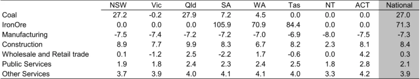
Overall labour supply is fixed in the model, so movements in employment are
effected through labour movements across industries and States.6 Coal and iron
ore capture the bulk of the labour movements (Table 2). The construction and
retail trade industries also gain labour while manufacturing see decreases in
employment.
Table 2: Industry (select) employment by State
NSW Vic Qld SA WA Tas NT ACT National
Coal 27.2 -0.2 27.9 7.2 4.5 0.0 0.0 0.0 27.0
IronOre 0.0 0.0 0.0 105.9 70.9 84.4 0.0 0.0 71.3
Manufacturing -7.5 -7.4 -7.2 -7.2 -7.0 -6.9 -8.0 -7.5 -7.3
Construction 8.9 7.7 9.9 8.3 6.7 8.2 2.3 8.1 8.4
Wholesale and Retail trade 0.1 -1.2 2.5 -2.2 1.7 -0.6 0.0 4.2 0.3
Public Services 1.9 1.8 2.4 2.3 2.4 2.5 1.8 2.8 2.1
Other Services 3.7 3.9 4.0 4.1 4.1 4.0 3.3 4.2 3.9
All results are presented as percentage changes. Source: Authors’ calculations.
Table 3: Employment and real consumer wage by State
NSW Vic Qld SA WA Tas NT ACT National
Employment -0.2 -0.7 0.9 -0.7 1.2 0.0 -1.5 1.9 0.0
Real wages 2.4 1.6 2.5 1.6 2.6 1.5 2.4 4.1 2.2
All results are presented as percentage changes. Source: Authors’ calculations.
Labour flows to the resource‐rich States of Western Australia and Queensland,
as well as the Australian Capital Territory, from the other States (Table 3).
The move towards more capital‐intensive sectors sees a fall in the cost of labour,
with the real producer wage falling by around 0.8 per cent. The real consumer
wage, however, captures the income effect of the higher terms of trade and
increases by around 2 per cent. This income effect is positive across all States
6 This, of course, is a strong assumption. It assumes that there is no further scope for
increased labour supply through higher workforce participation or increases in the
(Table 3) but largest in Western Australia, Queensland and the Australian Capital Territory.
Summary of results
The results show the same pattern of impacts across States and industries as
observed in the data to date, however the model suggests larger losers than we
have observed in manufacturing and the regions that depend the most on
manufacturing industries. The reallocation of resources suggested in the model
reflects the full employment assumption, with sectors expanding only through
drawing resources away from other sectors. In particular, the modelling implies
potentially significant movements of labour supply across industries and the
States. The implication is that if the recent rise in the terms of trade is sustained,
then the adjustment process from here may require a more significant
reallocation of resources than we have seen to date.
The results of the model, however, are comparative static and tell us little about the path of adjustment. It assumes that the supply of factors of production is fixed when in practice the supply potential of the economy can be expanded, for example through enhancing labour supply. The results pose a range of questions
as to how these adjustments may unfold in practice. The next section addresses
one of these questions — whether labour is sufficiently mobile across States to allow the employment changes suggested by the modelling results.
5.1 State labour markets and labour mobility
With the unemployment rate at generational lows and the participation rate
has been the case in well over three decades.7 The modelling results described in
the previous section suggest that structural adjustments associated with a
continued terms of trade boom would require significant movement of resources between the States in a full employment economy — more so than we have seen to date. In this sub‐section, we focus on the likely adjustments needed in the labour markets of Western Australia and Queensland assuming the higher terms of trade is sustained.
Employment growth in the resource‐rich States to date has been largely sourced
from within the States themselves. As a result, unemployment rates have fallen
well below the national average and participation rates have risen to around
record highs (Charts 12 and 13).
Chart 12: Unemployment rates
2 4 6 8 10
Mar-98 Mar-00 Mar-02 Mar-04 Mar-06 Mar-08 2 4 6 8 10
Western Australia Queensland Rest of Australia
Per cent Per cent
Source: ABS Labour Force Survey, Catalogue Number 6202.0.
Chart 13: Participation rates 60 62 64 66 68 70
Mar-98 Mar-00 Mar-02 Mar-04 Mar-06 Mar-08 60 62 64 66 68 70
Western Australia Queensland Rest of Australia
Per cent Per cent
Source: ABS Labour Force Survey, Catalogue Number 6202.0.
The ratio of full‐time equivalent employment to working age population is a
measure of labour utilisation that adjusts for the number of hours worked by
part‐time and full‐time workers. This measure is also at a generation high in the resource‐rich States (Chart 14).
Chart 14: Full-time equivalent employment to population ratio
46 48 50 52 54 56
Mar-80 Mar-84 Mar-88 Mar-92 Mar-96 Mar-00 Mar-04 Mar-08 46 48 50 52 54 56
Western Australia Queensland Rest of Australia
Per cent Per cent
Source: ABS Labour Force Survey, Catalogue Number 6202.0.
There is a question as to how much further the resource‐rich States can expand
are clear signs of wage pressures in Western Australia and Queensland, where unemployment rates have been driven below the national average.
The relationship between strong labour market outcomes and higher wage
inflation is illustrated in Chart 15, which presents a scatter plot of wage inflation
and unemployment rates for the resource‐rich States and the rest of Australia.
Wage pressures have increased in the resource‐rich States as their
unemployment rates have fallen below that of the rest of the country.
Chart 15: Wage growth and unemployment rate
2 3 4 5 6 3 4 5 6 7 8 9
Unemployment rate, per cent
Wage gr owt h , t ty 2 3 4 5 6 Resource-rich States Rest of Australia
Mar- 08
Mar-08 Mar-99
Mar-99
Per cent Per cent
Source: ABS Labour Force Survey and Labour Price Index, Catalogue Numbers 6202.0 ad 6345.0.
If the scope to expand internal labour markets is limited, then further
employment growth would need to be sourced from growth in the working age population. This can take two forms — increases in natural population growth or
higher immigration, either from overseas or interstate. As birth and death rates
are relatively stable and difficult to change in the short run, an expansion of labour supply would need to be sourced from higher immigration.
It is likely to be difficult to achieve large labour movements between the States to
meet additional demand from the resource‐rich States. The
Industry Commission (1993) found that, in the event of a state‐specific shock to
the labour market, changes in participation rates provided the major adjustment
mechanism, and interstate migration played a relatively minor role. That is,
when the unemployment rate in a State fell relative to the rest of the country, the
participation rate rose to restore the State’s relative unemployment rate. What
we have witnessed to date — rises in the participation rates in the two
resource‐rich States and little change in interstate migration — appears to be
consistent with this analysis.
Using a similar empirical framework, Debelle and Vickery (1998) found that
interstate migration does play an important role in the adjustment to
state‐specific shocks to the labour markets. They find that when a state labour
market is faced with a state‐specific shock, workers do move across state
boundaries, but the adjustment takes between four and seven years on average.
They also find that persistent differences remain between relative
unemployment rates between States.
We updated Debelle and Vickery’s analysis to take account of more recent data.
Our results show a larger response of average interstate migration to
Chart 16: Response of migration to employment shocks in Debelle and Vickery (1998) 0.00 0.05 0.10 0.15 0.20 0.25 0.30 0 5 10 15 20 25 30 35 40 45 50 0.00 0.05 0.10 0.15 0.20 0.25 0.30
Debelle and Vickery Update
Per cent Per cent
Note: The chart represents the per cent response of average interstate migration to a 1 per cent rise in employment (relative to the national average) over quarters from the shock (represented in the horizontal axis). In the original Debelle and Vickery paper, the shock resulted in a 0.19 per cent rise in average interstate migration in the long run. The updated analysis puts the magnitude of long-run rise in average interstate migration at about 0.28 per cent. Source: Authors’ calculations.
Both studies use the framework developed by Blanchard and Katz (1992) which
analyses labour market movements between US states.8 This analysis suggests
labour markets adjust through changes in unemployment rates rather than
relative wages. In Australia in the current boom, nominal wages in the
resource‐rich States have grown faster than in the rest of the country, bringing
about some change in relative wages. Chart 17 shows that the average wage in
Western Australia has risen above that of Victoria in 2004‐05, and that of
New South Wales in 2006‐07. The average wage level in Queensland remains the lowest among the four major States.
8 There are many interesting extensions that may be valuable to this area of research.
Including variables such as house prices is one simple extension that could be made to the current model. Another line of research would be to conduct a more micro‐based analysis regarding what drives internal migration. An inclusion of some measure of geographical isolation would be particularly interesting given the remote nature of many mining sites.
Chart 17: Wage level by state (AWOTE) 600 700 800 900 1000 1100 1200 1300
Mar-99 Mar-00 Mar-01 Mar-02 Mar-03 Mar-04 Mar-05 Mar-06 Mar-07 Mar-08 600 700 800 900 1000 1100 1200 1300
Western Australia Queensland New South Wales Victoria $ weekly earnings $ weekly earnings
Source: ABS Average Weekly Earnings, Catalogue Number 6302.0.
Chart 17 represents nominal wages, but what matters to workers is the real
wage. A spatial cost‐of‐living comparison is unfortunately not readily available. The relative increase in housing costs in Western Australia is one factor that may have offset relative real wage gains in that State (Chart 18).
Chart 18: Median house prices by capital cities
0 100 200 300 400 500 600
Mar-99 Mar-00 Mar-01 Mar-02 Mar-03 Mar-04 Mar-05 Mar-06 Mar-07 Mar-08 0 100 200 300 400 500 600
Perth Brisbane Sydney Melbourne
$000 $000
Source: Australian Property Monitors.
If wages have not adjusted sufficiently to draw significant amounts of labour
demand across the States as suggested by simple CGE models. At least, the
adjustment will not be as rapid or as costless as suggested by these models. An
alternative is that a higher proportion of the increase in population will be met
by overseas migration. But in practice the task of absorbing the required
immigration levels may raise significant policy challenges.
What is the likely magnitude of labour required by the resource‐rich States?
Consider the following scenario. In the three years since 2003‐04, employment
has grown annually by 3.8 per cent in Western Australia and 4.4 per cent in
Queensland. Suppose these two States were to record working age population
growth of the order required to maintain employment growth of the past three
years over the next three years. This would require the working age population
to rise by about 130,000 persons in Western Australia and 292,000 in Queensland
by 2010‐11. Assuming that the ratio of working age to total population in these
States remained constant over the next three years, this translates into a
population increase of about 161,000 persons in Western Australia and
367,000 persons in Queensland by 2009‐10.9
Western Australia’s population would need to grow by an average of around
36,000 persons per year beyond natural population growth. To put this number
in context, since 1981‐82, net interstate migration into Western Australia has
averaged around 2,000 persons per year and net overseas migration has
9 These are conservative estimates of the population growth required, as the scenario
assumes that all of the additional people in the working age population gain
employment. An alternative scenario would be to hold the unemployment and
participation rates for these States constant. To maintain employment growth under this
approach would require population growth of 250,000 persons in Western Australia and
averaged around 14,000 persons a year (rising dramatically in recent years to be nearly 26,000 in 2006‐07).
Queensland’s population would need to grow by an average of about
91,000 persons a year beyond natural growth. This compares with annual
average net interstate migration into Queensland of about 28,000 persons and
average net overseas migration of around 16,000 persons a year since 1981‐82
(net overseas migration reached a record high of nearly 34,000 in 2006‐07).
In practice, the potential labour market adjustments needed in the resource‐rich
States to accommodate a sustained rise in the terms of trade are likely to need to take place over a reasonably long time period. While an economy operating with
substantial unutilised capacity can grow employment relatively quickly,
reallocating resources or absorbing new labour through immigration will take
longer in a full employment economy. In the short term, competition for existing
labour supply could lead to significant wage pressures which would spill over
into broader inflationary pressures. This raises challenges for management of the macroeconomy in the short term.
6. P
OLICY IMPLICATIONS AND CONCLUSIONIt is clear from the above analysis that expanding labour supply in the
resource‐rich regions of the country will be a central policy challenge in
managing the transition to a higher terms of trade. While the gains from
increased participation may be reaching their limits in some States, the
Another possible response is for a significant amount of labour to be sourced
from net overseas migration. Net overseas migration has added 700,000 people
to the population in the past five years, and as many as another 350,000 are
projected to be added in the next two years — a net addition of more than
1 million migrants to a total population of 21 million. Clearly, there are limits to
how quickly these migrants can be absorbed into the economy given a broad
spectrum of issues encompassing housing demand, the provision of public
infrastructure and broader societal impacts. These issues will increasingly
require policy attention.
An emerging issue for policy makers is labour mobility within Australia. It is
unlikely that Australia can rely on mobility between the States to fully
equilibrate changing labour demands across regions. There will always be
natural barriers to labour mobility, such as the remoteness of Western Australia,
and the significant social adjustments associated with moving from one State to
another. That said, there are positive measures that may be taken to improve
labour mobility between States. Such an agenda could encompass measures to
address regulatory barriers to moving such as differences in schools systems and
occupational and business licensing arrangements. Cooperation between
different levels of government will be important for making progress on
harmonising standards across jurisdictions, and this is part of the agenda for the Council of Australian Governments.
Adjustment to a higher terms of trade will continue to present challenges for
monetary policy in a full employment economy (see Gruen, 2008 for a detailed
discussion). Fiscal policy can assist by allowing the ‘automatic stabilisers’ to
operate. Tighter fiscal policy does not reduce the total amount of restraint
it more widely and evenly, taking some pressure off interest rates and the exchange rate.
Assuming the terms of trade rise is sustained, there will be a structural
improvement in the Australian Government’s fiscal position. This will lead to
either higher budget surpluses over time or increases in spending/lower taxes to return the structural position of the budget back to its previous level in a way
that is consistent with the cyclical position of the economy. There are also
potential federal‐state financial issues, with higher incomes from the terms of
trade rises largely accruing to the federal budget, but cost pressures associated with physical infrastructure demands largely concentrated at the state level. It is also clear that with significant financial resources available, the Government will come under pressure to alleviate some of the adjustment costs on industries
and regions that are affected negatively by a higher terms of trade. However,
policies aimed at limiting sectoral and regional growth differentials by
supporting slower growing sectors would impede the reallocation of labour and
capital, putting further pressure on existing capacity. By increasing competition
for inputs, such policies would exacerbate inflationary pressures by further
driving up input prices across the country. Ultimately, this would shift more of
the burden of suppressing demand growth to other sectors not receiving
support. The challenge is to provide support in such a way as to aid the
necessary adjustment.
Current macroeconomic institutional arrangements mean we are better placed to
deal with the macroeconomic challenges of a rising terms of trade than in
implication that inflation expectations are much better anchored. A flexible exchange rate will help smooth fluctuations both on the way up and on the way
down from a terms of trade rise. Further structural reforms have improved the
flexibility of labour and product markets to adjust to external shocks.
The prospect of the rise in the terms of trade being sustained therefore need not
be considered a ‘resources curse’ that will simply create problems for policy
makers in managing its effects. If well managed, the transition to a higher terms
of trade presents an opportunity to raise Australian living standards. But the
challenges in ensuring a successful transition are significant and will test our policy frameworks in ways they have not been tested before.
7. B
IBLIOGRAPHYBlanchard, D and Katz, L 1992, ‘Regional Evolutions’, Brookings Papers on
Economic Activity, 1, pages 1‐61.
Commonwealth of Australia 2002, Budget Paper No. 1, Budget Strategy and
Outlook 2002‐03, Statement no. 4, Canberra.
Commonwealth of Australia 2006, Budget Paper No. 1, Budget Strategy and
Outlook 2006‐07, Statement no. 4, Canberra.
Commonwealth of Australia 2008, Budget Paper No. 1, Budget Strategy and
Outlook 2008‐09, Statement no. 2, Canberra.
Corden, M and Neary, J 1982, ‘Booming sector and de‐industrialisation in a small
open economy’, Economic Journal, 92 (December): 825‐848.
Corden, M 1984, ‘Booming sector and Dutch disease economics: survey and
consolidation’, Oxford Economic Papers, 36: 362.
Debelle, G and Vickery, J 1998, ‘Labour market adjustment: evidence on
interstate labour mobility’, RBA Discussion Paper, RDP 9801.
Dixon, P and Rimmer, M 1999 ‘MONASH: A Disaggregated Dynamic Model of
the Australian Economy: Technical Documentation’, Centre for Policy Studies
and IMPACT Project, Monash University, Melbourne.
Gregory, R 1976, ‘Some implications of the growth of the minerals sector’,
Gruen, D 2006, ‘A tale of two terms‐of‐trade booms’, Economic Roundup, Summer, pages 21‐34.
Gruen, D 2008, ‘The economic outlook’, speech to Australian Business
Economists, April.
Henry, K 2006, ‘Implications of China’s re‐emergence for the fiscal and economic
outlook’, Economic Roundup, Winter, pages 39‐58.
Industry Commission 1993, ‘An Empirical Assessment of Interstate Mobility and
Wage Flexibility’, Appendix D, in Impediments to Regional Adjustment, AGPS,
Canberra.
Kennedy, S 2007, ‘Full Employment in Australia and the Implications for Policy’, speech to the NSW Economic Society on 11 December.
Peter, M, Horridge, M, Meagher, G, Naqvi, F and Parmenter, B 1996, ‘The
Theoretical Structure of MONASH‐MRF’, Preliminary Working Paper no. OP‐85, Centre of Policy Studies, Monash University, Melbourne.
A
PPENDIXA
M
ODEL DESCRIPTIONThe MMRF model is from the Centre of Policy Studies at Monash University. It
is developed from the comparative static MMRF model (Peter et al 1996) and the dynamic, single‐region MONASH model (Dixon and Rimmer 1999).
The model has the following economic assumptions in the simulation set out in
this paper:
comparative static framework which compares the effect of the price
rise against a base case of unchanged prices;
supply and demand behaviour determined via market clearing
conditions;
overall labour supply is fixed, and labour mobility is achieved through
the movement in unemployment rates between jurisdictions;
capital supply is both fixed and immobile;
industry capital stocks do not adjust;
government expenditure rises broadly in line with increases in
revenue.
The model estimates the impact of the negotiated contract price increases from
2003‐04 to 2006‐07 for coal and iron ore.
Consistent with the theory underpinning the MMRF model, to calibrate the
increase by 48 per cent, iron ore prices by 123 per cent, coal export volumes by 5 per cent and iron ore export volumes by 32 per cent. These percentage changes are modelled as commodity‐specific shifts in foreign export demand curves.
Some of the limitations with the model and the assumptions adopted are
outlined below.
With the short‐run assumption that industry capital stocks remain constant, this
implies that investment is unchanged in the short‐run, which is not necessarily
consistent with the current strong growth in business investment. The model is
also comparatively rigid in that it is less capable of capturing substitution effects
in the economy, due to the Leontief nested structure at the top nest production
function. Therefore for some industries, inputs are combined in fixed
proportions (Leontief production technology) to produce output with the
elasticity of substitution being zero. For other industries, the value of elasticity is
non‐zero and therefore a constant elasticity of substitution technology is
imposed. For example, companies can not substitute away from iron ore and
coal as inputs to production. Changes in consumer tastes/preferences are also
not captured in the results.