Anisotropic adaptive kernel deconvolution
Fabienne Comte, Claire Lacour
To cite this version:
Fabienne Comte, Claire Lacour. Anisotropic adaptive kernel deconvolution. Annales de l’Institut Henri Poincar´e (B) Probabilit´es et Statistiques, Institute Henri Poincar´e, 2013, 49 (2), pp.569-609. <10.1214/11-AIHP470>. <hal-00579608v2>
HAL Id: hal-00579608
https://hal.archives-ouvertes.fr/hal-00579608v2
Submitted on 12 Dec 2011
HAL is a multi-disciplinary open access archive for the deposit and dissemination of sci-entific research documents, whether they are pub-lished or not. The documents may come from teaching and research institutions in France or abroad, or from public or private research centers.
L’archive ouverte pluridisciplinaire HAL, est destin´ee au d´epˆot et `a la diffusion de documents scientifiques de niveau recherche, publi´es ou non, ´emanant des ´etablissements d’enseignement et de recherche fran¸cais ou ´etrangers, des laboratoires publics ou priv´es.
F. COMTE(∗) AND C. LACOUR(∗∗)
Abstract. In this paper, we consider a multidimensional convolution model for which we
provide adaptive anisotropic kernel estimators of a signal density f measured with additive error. For this, we generalize Fan’s (1991) estimators to multidimensional setting and use a bandwidth selection device in the spirit of Goldenshluger and Lepski’s (2011) proposal for density estimation without noise. We consider first the pointwise setting and then, we study the integrated risk. Our estimators depend on an automatically selected random bandwidth. We assume both ordinary and super smooth components for measurement errors, which have known density. We also consider both anisotropic Hölder and Sobolev classes forf. We provide non asymptotic risk bounds and asymptotic rates for the resulting data driven estimator, together with lower bounds in most cases. We provide an illustrative simulation study, involving the use of Fast Fourier Transform algorithms. We conclude by a proposal of extension of the method to the case of unknown noise density, when a preliminary pure noise sample is available.
Résumé. Dans ce travail, nous considérons un modèle de convolution multidimensionnel, pour lequel nous
proposons des estimateurs à noyau anisotropes pour reconstruire la densitéf d’un signal mesuré avec un bruit additif. Pour ce faire, nous généralisons les estimateurs de Fan (1991) à un contexte multidimensionnel et nous appliquons une méthode de sélection de fenêtre dans l’esprit des idées récentes développpées par Goldenshluger et Lepski (2011) pour l’estimation de densité en l’absence de bruit. Nous considérons tout d’abord le problème de l’estimation ponctuelle, et nous étudions ensuite le risque global intégré. Nos estimateurs dépendent d’une fenêtre aléatoire sélectionnée de façon automatique. Nous considérons les cas où les composantes du bruit, supposées con-nues, peuvent être ordinairement ou super régulières. De plus, nous étudions des classes de fonctionsf à estimer aussi bien dans des espaces de Hölder anisotropes que dans des espaces de Sobolev. Nous prouvons des bornes de risque non asymptotiques ainsi que des vitesses de convergence asymptotiques pour nos estimateurs adaptatifs, en même temps que des bornes inférieures dans un grand nombre de cas. Des simulations illustrent la méthode en s’appuyant sur des algorithmes de transformation de Fourier rapide. En conclusion, nous proposons une extension de la méthode lorsque la loi du bruit n’est plus connue, mais remplacée par un échantillon préliminaire où le bruit seul est observé.
(*)University Paris Descartes, Sorbonne Paris Cité, MAP5 UMR CNRS 8145
(**)University Paris-Sud 11, Laboratoire de Mathématique d’Orsay
Keywords. Adaptive kernel estimator. Anisotropic estimation. Deconvolution. Density esti-mation. Measurement errors. Multidimensional.
Primary subjects. 62G07.
1. Introduction
There have been a lot of studies dedicated to the problem of recovering the distribution f
of a signal when it is measured with an additive noise with known density. Several strategies have been proposed since Fan [1991] in order to provide adaptive strategies for kernel (Delaigle and Gijbels [2004]) or projection (Pensky and Vidakovic [1999], Comte et al. [2006]) estimators. The question of the optimality of the rates revealed real difficulties, after the somehow classical cases studied by Fan [1991]: the case of super smooth noise (i.e. with exponential decay of its characteristic function) in presence of possibly also super smooth density implies non standard
bias variance compromises that require new methods for proving lower bounds. These problems have been studied by Butucea [2004], Butucea and Tsybakov [2008a,b] and by Butucea and Comte [2009].
Then new directions lead researchers to release the assumption that the characteristic function of the noise never vanishes, see Hall and Meister [2007], Meister [2008]. Others released the assumption that the density of the noise is known. In physical contexts, where it is possible to obtain samples of noise alone, a solution has been proposed by Neumann [1997], extended to the adaptive setting by Comte and Lacour [2011], another idea is developed in Johannes [2009]. Other authors assumed repeated measurements of the same signal, and proposed estimation strategy without noise sample, see Delaigle et al. [2008].
All these works are in one dimensional setting. Our aim here is to study the multidimensional setting, and to propose adaptive strategies that would take into account possible anisotropy for both the function to estimate and the noise structure. As already explained in Kerkyacharian et al. [2001], adaptive procedures are delicate in a multidimensional setting because of the lack of natural ordering. For instance, the model selection method is difficult to apply here since it requires to bound terms on sums of anisotropic models. In this paper, we use a unified setting where all estimators can be seen as kernel estimators, and we use the method recently developed in Goldenshluger and Lepski [2010, 2011] to face anisotropy problems. The originality of our work is to use Talagrand inequality as the key of the deviation in the mean squared error case. This idea is also exploited in a different context by Doumic et al. [2011]. And indeed, we succeed in building adaptive kernel estimators in many contexts. The bandwidth is automatically selected. We provide risk bounds for these estimators, for both pointwise risk when local bandwidth selection is proposed and for the integrated mean square risk (MISE) when the global selection is studied. We also consider both anisotropic Hölder and Sobolev classes forf, the Fourier-domain-definition of the last ones allowing to also deal with the case of super smooth functions. Few papers study the multidimensional deconvolution problem; we can only mention Masry [1991] who considers mainly the problem of dependency between the variables without anisotropy nor adaptation, and Youndjé and Wells [2008] who consider a cross-validation method for bandwidth selection in an isotropic and ordinary smooth setting. Our paper considerably generalizes their results with a different method, and provides new results and new rates in both pointwise and global setting.
We want here to emphasize that our setting is indeed very general. We consider all possible cases: the noise can have both ordinary smooth (O.S.) components (i.e. a characteristic function with polynomial rate of decay in the corresponding directions) and super smooth (S.S.) compo-nents (exponential rate of decay), and the signal density also. In particular, we obtain surprising results in the mixed cases: if one component only of the noise is S.S. (all the others being O.S.), in presence of an O.S. signal, then the rate of convergence of the estimator is logarithmic. On the contrary, if the signal hask out ofdcomponents S.S. in presence of an O.S. noise, then the rate of the estimator is almost as good as if the dimension of the problem was d−kinstead ofd. We obtain also natural extensions of the univariate rates, and in particular the important fact that the rates can be logarithmic if the noise is S.S. (for instance in the Gaussian case) but are much improved if the signal is also S.S.: for instance, if the signal is also Gaussian, then polynomial rates are recovered.
In spite of the difficulty of the problem, in particular because of the large number of parameters required to formalize the regularity indexes of the functions, we exhibit very synthetic penalties than can be used in all cases. We also provide more precise but more technical results. It is certainly worth mentioning that the adaptive strategy we propose in the pointwise setting is not only a generalization of the one-dimensional results obtained in Butucea and Comte [2009],
but is also a different procedure. Lastly, we prove original lower bounds for both pointwise and global setting, and this requires specific constructions.
The plan of the paper is the following. In Section 2, we describe the model and the assumptions: the functional classes and the kernels used in the following. We both give the conditions required in the following for the kernels and provide concrete examples of kernels fulfilling them. We define the general estimator by generalization of the one-dimensional kernel to multidimensional setting. In Section 3, we study the pointwise risk and we discuss the rates. We also assert the optimality of most rates by proving lower bounds. Then we propose a pointwise bandwidth selection strategy and prove risk bounds for the estimator in the case of Hölder classes and for Sobolev classes. As in the univariate case, adaptation costs a logarithmic loss in the rates. In Section 4, we provide global (upper and lower) MISE bounds and describe an adaptive estimator, which is studied both on Nilkols’kii (see Nikol’ski˘ı [1975] and Kerkyacharian et al. [2001]) classes and for Sobolev densities. Here, it is possible that adaptation has no price and that the rate corresponds exactly to the optimal one found without adaptation. We provide in Section 5 illustrations and examples in dimension 2, for models having possibly very different behavior in the two directions. We give results of a small Monte-Carlo study, obtained by clever use of IFFT to speed the programs. Up to our knowledge, these effective experiments are the first ones in such a general setting. In a concluding Section 6, we pave the way for a generalization of the method to the case where the known noise density is replaced by an estimation based on a preliminary sample. To finish, all proofs are gathered in Section 7.
2. Model, estimator and assumptions.
2.1. Model and notations. We consider the following d-dimensional convolution model
(1) Yi = Yi,1 .. . Yi,d =Xi+εi = Xi,1 .. . Xi,d + εi,1 .. . εi,d , i= 1, . . . , n.
We assume that the εi and theXi are i.i.d. and the two sequences are independent. Only the
Yi’s are observed and our aim is to estimate the densityf ofX1when the densityfεofεis known.
As far as possible, we shall denote byx variables in the time domain and by tor u variables in the frequency domain. We denote by g∗ the Fourier transform of an integrable function g,
g∗(t) =R eiht,xig(x)dx where ht, xi=Pdj=1tjxj is the standard scalar product inRd. Moreover
the convolution product of two functionsg1 andg2is denoted byg1⋆ g2(x) =R g1(x−u)g2(u)du.
We recall that (g1⋆ g2)∗=g1∗g∗2. As usual, we define
kgk1= Z |g(x)|dx and kgk=kgk2 = Z |g(x)|2dx 1/2 .
The notation x+ means max(x,0), and a≤bfor a, b∈Rd means a1 ≤b1, . . . , ad≤bd. For two
functions u, v, we denote u(x) . v(x) if there exists a positive constant C not depending on x
such that u(x)≤Cv(x) and u(x)≈v(x) if u(x).v(x) and v(x).u(x).
2.2. The estimator. Let us now define our collection of estimators. LetKbe a kernel inL2(Rd)
such that K∗ exists. Then we define, for h∈(R∗+)d,
Kh(x) = 1 h1. . . hd K x1 h1 , . . . ,xd hd and L∗(h)(t) = Kh∗(t) f∗ ε(t) .
The kernelK is such that Fourier inversion can be applied:
L(h)(x) = (2π)−d
Z
e−iht,xiKh∗(t)/fε∗(t)dt, if fε∗(t)6= 0.
Considering that fY =f ⋆ fε and thusf∗ =fY∗/fε∗, a natural estimator off is such that
ˆ fh∗(t) =fc∗ Y(t)L∗(h)(t) =Kh∗(t) c fY∗(t) f∗ ε(t) , where fc∗ Y(t) = 1 n n X k=1 eiht,Yki,
provided thatfε∗ does not vanish, and thus, by Fourier inversion,
ˆ fh(x) = 1 n n X k=1 L(h)(x−Yk).
Note that our estimator here is the same, in multivariate context, as the one proposed in one-dimensional setting by Fan (1991). It verifies
E( ˆfh∗(t)) =Kh∗(t)fY∗(t)
fε∗(t) =Kh∗(t)f∗(t) so that E( ˆfh) =Kh⋆ f =:fh.
To construct an adaptive estimator, we also introduce auxiliary estimators involving two kernels. This idea, already used in Devroye [1989], allows us in the following to automatically select the bandwidthh(see section 3.4), following a method described in Goldenshluger and Lepski [2011]. We consider
ˆ
fh,h′(x) =Kh′⋆fˆh(x), which implies that
ˆ fh,h∗ ′(t) =Kh∗′(t)Kh∗(t) c fY∗(t) f∗ ε(t) .
Note that, for all x ∈Rd, we havefˆh,h′(x) = ˆfh′,h(x). The estimator which is finally studied is
ˆ
fˆh where ˆhis defined by using the collection ( ˆfh,h′).
2.3. Noise assumptions. We assume that the characteristic function of the noise has a poly-nomial or exponential decrease:
(Hε) ∃α ∈(R+)d, ρ∈(R+)d, β ∈Rd(βj >0 if ρj = 0)s. t. ∀t∈Rd, |fε∗(t)| ≈ d Y j=1 (t2j + 1)−βj/2exp(−α j|tj|ρj).
Note that this assumption implies fε∗(t) 6= 0, ∀t ∈ Rd. A component j of the noise is said to be ordinary smooth (OS) if αj = 0 or ρj = 0 and super smooth (SS) otherwise. We take the
convention that αj = 0 if ρj = 0and ρj = 0 ifαj = 0.
Let us recall that exponential or gamma type densities are ordinary smooth, and that Cauchy or Gaussian densities are super smooth. The Gaussian case is considered in many problems and enhances the interest of super smooth contexts. But exponential-type densities keep a great interest in physical contexts, see for instance the fluorescence model studied in Comte and Rebafka [2010] where the measurement error density is fitted as an exponential type distribution, belonging to the ordinary smooth class.
To be more precise, we introduce the following notation. We denote byOS the set of directions
j with ordinary smooth regularity (αj =ρj = 0), and by SS the set of directions j with super
smooth regularity (ρj >0) so that under(Hε),
|fε∗(t)| ≈ Y j∈OS (t2j + 1)−βj/2 Y k∈SS (t2k+ 1)−βk/2exp(−α k|tk|ρk).
2.4. Regularity assumptions. We consider in the sequel several types of regularity for the target functionf, associated with slightly different definition of the estimator: the choice of the kernel depends on the type of regularity space. We used Greek letters for the noise regularity, and now, we use Latin letters for the functionf regularity indexes.
First, for pointwise estimation purpose, we consider functions f belonging to Hölder classes denoted byH(b, L),b= (b1, . . . , bd) such that:
the function f admits derivatives with respect to xj up to order ⌊bj⌋ (where ⌊bj⌋ denotes the
largest integer less thanbj) and
∂⌊bj⌋f (∂xj)⌊bj⌋ (x1, . . . , xj−1, x′j, xj+1, . . . , xd)− ∂⌊bj⌋f (∂xj)⌊bj⌋ (x) ≤L|x ′ j−xj|bj−⌊bj⌋.
Next for global estimation purpose, the functional spaces associated with standard kernel estimators are the anisotropic Nikol’skii class of functions, as in Goldenshluger and Lepski [2010], see also Nikol’ski˘ı [1975], Kerkyacharian et al. [2001]. We consider the classN(b, L) which is the set of functions f :Rd →Rsuch that f admits derivatives with respect toxj up to order ⌊bj⌋,
and
(i) k ∂⌊
bj⌋f
(∂xj)⌊bj⌋k ≤
L, for all j= 1, . . . , d, where k.k denotes theL2(Rd)-norm.
(ii) For all j= 1, . . . , d, for allt∈R,
Z ∂⌊bj⌋f (∂xj)⌊bj⌋ (x1, . . . , xj−1, xj+y, xj+1, . . . , xd)− ∂⌊bj⌋f (∂xj)⌊bj⌋ (x) 2 dx≤L2|y|2(bj−⌊bj⌋).
Lastly, and for both pointwise and global estimation, we shall consider general anisotropic Sobolev spacesS(b, a, r, L) defined as the class of integrable functions f :Rd→Rsatisfying
d
X
j=1
Z
|f∗(t1, . . . , td)|2(1 +t2j)bjexp(2aj|tj|rj)dt1. . . dtd≤L2,
for aj ≥ 0, rj ≥ 0, bj ∈ R, when j = 1, . . . , d. We set aj = 0 if rj = 0, and reciprocally, and
in this case, bj > 1/2 (otherwise bj ∈ R). If someaj are nonzero, the corresponding directions
are associated with so-called "super smooth" regularities. To standardize notations, we set
aj =rj = 0when Hölder or Nikol’skii regularity is considered.
We refer to Triebel [2006] for definitions and comparison of these spaces with other type of anisotropic regularity spaces such as Besov spaces.
We can note that Sobolev spaces allow one to take into account a global regularity rather than a pointwise one. Nevertheless, they have a convenient Fourier-domain representation, in particular when one wants to consider super smooth or analytical functions, even in pointwise setting. If the noise density can have such property in the case of Gaussian measurement error, it is natural to think that the signal density may have the same behavior.
2.5. Assumptions on the kernel. For the estimators to be correctly defined, the kernel must be chosen sufficiently regular to recover integrability in spite of the noise density.
We assume thatK(x) =K(x1, . . . , xd) =Qdj=1Kj(xj). This assumption is not necessary, but
simplifies the proofs. Besides, the kernels used in practice verify this condition. Moreover, we recall that K belongs toL2(Rd) and admits a Fourier transform.
To ensure the finiteness of the estimators, we shall use the following assumption:
Kvar(β) Forj∈OS: R |K∗
j(u)|2(1 +u2)βjdu <∞ and
R |K∗
j(u)|(1 +u2)βj/2du <∞
Forj∈SS: Kj∗(t) = 0 if |t|>1 and sup|t|≤1|Kj∗(t)|<∞
Moreover, we may require a classical assumption to control the bias for functions in Hölder or Nikol’skii spaces described above.
Korder(ℓ) The kernelK is of order ℓ= (ℓ1, . . . , ℓd)∈Rd+, i.e.
∗ R K(x)dx= 1
∗ ∀1≤j ≤d,∀1≤k≤ℓj,
R
xkjK(x)dx= 0
∗ ∀1≤j ≤d,R(1 +|xj|)ℓj|K(x)|dx <∞
Note that this implies condition (A2) used in Fan [1991] which is stated in the Fourier domain. Condition Korder(ℓ) is verified by the following kernels defined in Goldenshluger and Lepski [2010]. We start by defining univariate functions uj(x) such that
R uj(x)dx = 1, R |x|ℓj|u j(x)|dx <+∞ and then (2) Kj(xj) = ℓj X k=1 ℓj k (−1)k+11 kuj( xj k).
ThenKj is a univariate kernel of order ℓj. The multivariate kernel is defined by
(3) K(x) =K(x1, . . . , xd) = d
Y
j=1
Kj(xj).
The resulting kernel is such that R Qdj=1xkj
j K(x)dx1. . . dxd = 0 if 1 ≤ kj ≤ ℓj for one j ∈
{1, . . . , d}, and thus satisfies Korder(ℓ).
We can give an example of kernel satisfying Assumptions Kvar(β) and Korder(ℓ). We can use the construction above with uj(xj) =vℓj+2(xj) where
vp(x) =cp sin(x/p) x/p p , vp(0) =cp, vp∗(t) = 2πpcp 2p |1[−1,1]⋆· · ·{z ⋆1[−1,1]} p times (pt),
andcp is such thatRvp(x)dx= 1. This is what can be done when the function under estimation
is assumed to be in a Hölder or in a Nikol’skii space.
When considering Sobolev space, since Assumption Kvar(β) only is required, we simply use the sinus cardinal kernel denoted by K= sincand defined by
Kj∗(t) =1[−1,1](t) =v1∗(t), Kj(xj) = sin(xj) πxj , Kj(0) = 1 π.
Remark. When only ordinary smooth noises are considered on Hölder or Nikol’skii spaces, we may also use other type of kernels. For instance, the construction of kernel of orderℓbased on
uj(xj) =cj xj− 1 2 ⌊βj⌋+1 xj+ 1 2 ⌊βj⌋+1 1[−21, 1 2](xj)
would suit. Indeed, it can be proved thatK∗
j(tj) =O(|tj|−(⌊βj⌋+2)) when |tj| →+∞.
3. Pointwise estimation
3.1. Bias and variance. Letx0 be a point in Rd. We aim to study the risk of the estimator
ˆ
fh off at point x0: |f(x0)−fˆh(x0)|. Recall thatfh =E( ˆfh) =Kh⋆ f and that
E|f(x0)−fˆh(x0)|2 =|f(x0)−fh(x0)|2 | {z } bias +E|fh(x0)−fˆh(x0)|2 | {z } variance .
We first control the bias. We define
B0(h) =
(
kf −fhk∞ if kKk1<∞
kf∗−fh∗k1/(2π)d otherwise
We recall that, when considering all types of spaces (Hölder and Sobolev), we standardized notations by settingaj =rj = 0when Hölder regularity is considered. The following proposition
holds.
Proposition 1. The bias verifies |f(x0)−fh(x0)| ≤B0(h) and, under assumptions
• f belongs to Hölder class H(b, L) and the kernel verifies Korder(ℓ) with ℓ≥ ⌊b⌋, or
• f∗ ∈L1(R),f belongs to Sobolev class S(b+ 1/2, a, r, L) and K= sinc, Then B0(h).LPdj=1hjbj+rj/2exp(−ajh−jrj).
Thus, we recover the classical order hbj
j when aj = 0. Let us now study the variance of
estimators fˆh.
Proposition 2. The variance verifies E|fh(x0)−fˆh(x0)|2 ≤V0(h) where
(4) V0(h) = 1 (2π)2d 1 nmin kf ∗ εk1 K∗ h fε∗ 2 2 , K∗ h fε∗ 2 1 ! .
Moreover, under (Hε) and Kvar(β), if hj ≤1 for all j,
V0(h). 1 n d Y j=1 h(ρj−1)++ρj−1−2βj j exp(2αjh−jρj).
Whenfε∗ = 1 (no noise), we obtain the classical orderQj1/(nhj).
Eventually, the bound on the MSE is obtained by adding the squared bias bound and the variance bound.
3.2.1. Homogeneous cases. We first give the bandwidth choices and rates of convergence which are obtained when all components of both f and fε have the same type of smoothness (all OS
or all SS). Recall that in dimension 1, the minimax rates are logarithmic when the noise is super smooth, unless the functionf is super smooth too : see Fan [1991], Pensky and Vidakovic [1999], Comte et al. [2006].
First, consider that both the functionf and the noise are ordinary smooth. We can compute the anisotropic rate that can be deduced from a "good" choice of h = (h1, . . . , hd). Indeed,
setting the gradient of h2b1
1 +· · ·+h2dbd+n−1
Qd i=1h−
(2βi+1)
i w.r.t. h to zero, we easily obtain
h2bj
j,opt=h
2bk
k,opt. Therefore the optimal bandwidth choice to minimize the risk bound is
(5) hj,opt∝n−1/(2bj+bj
Pd
i=1[(2βi+1)/bi])
and the resulting rate is proportional to
(6) ψn=n−1/(1+ 1 2 Pd i=1 2βi+1 bi ).
Secondly, consider the case where the noise is super smooth (all (βj, ρj) nonzero) but the
function is ordinary smooth. Then hj,opt= ((2αj+ 1)/log(n))1/ρj and the rate is of order
(7) ψn= [log(n)]−2 min1≤j≤d(bj/ρj).
We can remark two things in this case: the rates are logarithmic, and the bandwidth choice is known because it only depends on the parameters of the noise density, which is assumed to be known. This explains why no bandwidth selection procedure is required here, as long as only classical Hölder regularities are considered for f.
Now consider the case where the noise is ordinary smooth (all ρj’s are zeros) but the function
is super smooth (with all(aj, rj)nonzero). Then we takehj,opt= (aj/log(n))1/rj and the rate is
(8) ψn= [log(n)]
Pd
j=1(2βj+1)/rj/n.
We can see that here, the rates are very good. It is worth mentioning that the first paper considering super smooth functionf is Pensky and Vidakovic [1999].
We do not give a general bandwidth choice in the case where both functions can be super smooth, because it is very intricate. General formula in dimension 1 are given in Lacour [2006], see also Butucea and Tsybakov [2008a,b]. We can just emphasize that in such case the rates can be considerably improved, compared to the logarithmic issue above. We give an example below.
Super Smooth f/Super Smooth fε example. For instance, it is easy to see that the
compro-mise between a bias of order exp(−1/h2) and a variance of order exp(1/h2)/n is obtained for
h = p2/log(n) and gives a rate of order 1/√n. To be even more precise, the optimal rate in dimension 1, if the signal isN(0, σ2)and the noise N(0, σ2ε), isn−1/(1+θ2)[log(n)]−(1+1/(1+θ2))/2,
θ2 =σ2
ε/σ2, for 1/hopt=
p
[log(n) + (1/2) log(log(n))]/(σ2 +σ2
ε).
As the bandwidth choice is very difficult to describe in the general case, this enhances the interest of automatic adaptation which is proposed below, when Sobolev spaces are considered. Note that optimal choices of the bandwidth are of logarithmic orders in all those cases.
3.2.2. Discussion about mixed cases. Let us consider now the case where the function is still ordinary smooth, but components 1 to j0 of the noise are ordinary smooth while components
j0 + 1 to d are super smooth, 1 ≤ j0 < d. Then it is clear that exponential components
additively in the bias term, the rate becomes logarithmic. More precisely, taking forj= 1, . . . , j0,
hj,opt ∝n−1/(2d(2βj+1)) and for j =j0+ 1, . . . , d, hj,opt = [log(n)/(4dαj)]−1/ρj gives a variance
term of order n−1 j0 Y j=1 h−2βj−1 j,opt d Y j=j0+1 h(ρj−1)++(ρj−1)−2βj j,opt exp(2αjh− ρj j,opt) ∝ n−1+j0/(2d)+(d−j0)/(2d)logω(n) =n−1/2logω(n),
where ω =Pdj=j0+1(2βj + 1−ρj−(ρj−1)+)/ρj.Therefore, the variance is negligible and the
rate is determined by the bias terms and is proportional to (9) ψn= [log(n)]−2 minj0+1≤j≤d(bj/ρj).
The conclusion is that the presence of one super smooth component of the noise implies a loga-rithmic rate, when the function to estimate is ordinary smooth (and bandwidth selection is not required).
The other case we can handle is when the noise has all its components ordinary smooth, but the function has its j0 first components ordinary smooth and the d−j0 last ones super smooth.
Let us taked= 2 andj0 = 1for simplicity. Clearly, we can choose h2,opt= (log(n)/a2)−1/r2, so
that the MSE for (h1,opt, h2,opt) is proportional to
h2b1
1,opt+h22b,opt2+r2exp(−2a2h−2,optr2 ) +n−1h−
2β1−1 1,opt h− 2β2−1 2,opt ∝ h2b1 1,opt+n−2[log(n)]−(2b2+r2)/r2+n−1h− 2β1−1 1,opt [log(n)](2β2+1)/r2.
Therefore, the optimal choice of h1 is obtained as in dimension 1 with respect to a sample
size n/[log(n)](2β2+1)/r2 and we findh
1,opt ∝(n/[log(n)](2β2+1)/r2)−1/(2β1+2b1+1). The final rate
is proportional to (n/[log(n)](2β2+1)/r2)−2b1/(2β1+2b1+1). This is the rate corresponding to the
one-dimensional problem, up to a logarithmic factor. In the general case, we obtain a rate proportional to (10) ψn= n/ d Y j=j0+1 (logn) 2βj+1 rj −1/(1+12Pj0 i=1 2βi+1 bi )
In other words, we obtain in dimensiond, the rate corresponding to dimension j0 of the OS-OS
problem, up to logarithmic factors.
3.3. Lower bounds. To get a validation of our method, we need to prove lower bounds for the rates computed above, at least in part of the cases. In particular, we can extend the results of Fan [1991] and of Butucea and Tsybakov [2008b] to the multivariate setting. Our next result is not straightforward and requires specific constructions, since it captures mixed cases which could not be encountered in univariate setting.
Theorem 1. We assume that the noise has its components independent. We also assume that, for j= 1, . . . , d, and for almost all uj in R, fε∗1,j(uj) admits a derivative and
(11) |uj|β ′ jexp(α j|uj|ρj)|(fε∗1,j) ′(u j)|is bounded, for a constant β′
Case A: For j = 1, . . . , d, the components εj are ordinary smooth, D = H(b, L) or D =
S(b+ 1/2, a, r, L) with rj < 2, and if 1 ≤ rj < 2, fε∗1,j(uj) admits in addition a
sec-ond order derivative for almost all uj in R such that|uj|β
′′
j exp(α
j|uj|ρj)|(fε∗1,j)′′(uj)| is
bounded, with β′′j a positive constant. or
Case B: There exists at least one component ofεwhich is super smooth andD=H(b, L) or D=
S(b+ 1/2,0,0, L).
Then for any estimator fˆn(x0), and for nlarge enough,
sup f∈DEf h ( ˆfn(x0)−f(x0))2 i %ψn
where ψn is defined by (6) in Case A and D = H(b, L), by (10) in Case A and D = S(b+
1/2, a, r, L) with all rj’s less than 2, and by (9) in Case B.
Note that our condition on the noise improves Fan [1991]’s conditions: in the OS case, Fan requires a second order derivative offε∗ and in the SS case, he gives a technical condition which is difficult to link with the functions at hand. The improvement took inspiration in the book of Meister [2009] who also had first order type conditions.
We therefore conclude that the rates reached by our estimators for estimating an ordinary smooth function or a super smooth function if the noise is ordinary smooth, are optimal. We also have optimality in the case of an ordinary smooth functionf and super smooth noise. 3.4. Adaptive estimator. Now, our aim is to automatically select a bandwidth in a discrete set
H0 (described below) such that the corresponding estimator reaches the minimax rate, without
knowing the regularity of f. We may also ignore if f is ordinary or super smooth, or partially both, depending on the direction.
3.4.1. General result. We have at our disposal estimators fˆh(x0) and fˆh,h′(x0) = Kh′ ⋆fˆh(x0), for x0 = (x0,1, . . . , x0,d)∈Rd such thatfˆh,h′(x0) = ˆfh′,h(x0). We define
(12) A0(h, x0) = sup h′∈H0 |fˆh′(x0)−fˆh,h′(x0)| − q ˜ V0(h′) + , and ˆ h(x0) = arg min h∈H0 A0(h, x0) + q ˜ V0(h) with (13) V˜0(h) =c0log(n)V0(h)
and c0 is a numerical constant to be specified later. The final estimator is f˜(x0) = ˆfhˆ(x0)(x0).
The term V˜0(h) corresponds to the variance of the estimate fˆh(x0) multiplied by log(n). Now,
we can state the result concerning the adaptive estimator. Define
N(K) =
(
kKk1 if kKk1 <∞
Theorem 2. Assume that N(K)<∞ and let H0 = {h(k) s.t. h(jk)≤1, forj = 1, . . . , d, V0(h(k))≤1, Kh∗(k) f∗ ε 2 2 Kh∗(k) f∗ ε −2 1 ≥ log(nn) for k= 1, . . . ,⌊nǫ⌋}. (14)
Let q be a real larger than 1. Assume that c0 ≥(4(1 +kK∗k∞)(2ǫ+q))2/min (kfε∗k1,1).Then,
with probability larger than1−4n−q,
(15) |f˜(x0)−f(x0)| ≤ inf h∈H0 (1 + 2N(K))B0(h) + 3 q ˜ V0(h) .
We can make two comments about this result.
(1) Inequality (15) is a trajectorial oracle inequality, up to thelog(n)factor in the termV˜0(h)
which appears in place of V0(h).
(2) Condition (14) is typically verified ifkK∗
h/fε∗k22 ≥log(n)andmax(kKh∗/fε∗k22,kKh∗/fε∗k21)≤
n. It is just slightly stronger than assuming the variance V0(h) bounded.
It is also important to see that we can deduce from Theorem 2 a mean oracle inequality. More precisely, we have|f˜(x0)−f(x0)| ≤(kKh∗/fε∗k1+|f(x0)|). Then, forh∈ H0,kKh∗/fε∗k21 ≤
(n/log(n))kK∗
h/fε∗k22andV0(h)≤1implykKh∗/fε∗k21 ≤n. Thus|f˜(x0)−f(x0)|2 .n. Therefore,
Theorem 2 implies that,∀h∈ H0,
(16) E(|f˜(x0)−f(x0)|2)≤ (1 + 2N(K))B0(h) + 3 q ˜ V0(h) 2 + C n,
provided that we choose q≥2 in Theorem 2.
3.4.2. Study of Condition (14). Let us define¯hopt = (¯h1,opt, . . . ,¯hd,opt)the minimizer of the right
hand side of equation (16):
¯
hopt= arg min h∈Rd+
n
B02(h) + ˜V0(h)
o .
Note that¯hopt here corresponds to the value ofhopt computed in Section 3.2 wherenis replaced
by n/log(n). We need to check that ¯hopt belongs to H0 to ensure that the infimum in (15) is
reached.
This is what is stated in the following Corollary.
Corollary 1. Assume that (Hε) holds and either
1. f belongs to Hölder class H(b, L), the noise has all its components OS and the kernel verifies Korder(ℓ) with ℓ ≥ ⌊b⌋, Kvar(β), and is such that Kj∗ is lower bounded on
[−qj, qj]for qj >0, andj= 1. . . , d, or
2. f∗ ∈L1(R),f belongs to Sobolev class S(b+ 1/2, a, r, L) and K= sinc. Then ¯hopt∈ H0 defined by (14) and thus the infimum in Inequality (15) is reached.
In particular in case 1., we have
(17) E(|f˜(x0)−f(x0)|2) =O((n/log(n))−1/(1+ 1 2 Pd i=1 2βi+1 bi )).
We can notice that the proof of Corollary 1 relies on the intermediate result stating that Condition (14) is equivalent to the following one:
(18) d Y j=1 h(ρj−1) j .n/log(n).
The consequence of Corollary 1 is that the right hand side of (15) always leads to the best compromise between the squared bias B2
0(h) and V˜0(h), that is the optimal rates of section 3.2
with respect to a sample sizen/log(n).
Remark 1. As we already mentioned, we have an extra log(n) factor in Inequality (15). In case 1. above, we can concretely see the loss in the rate by comparing the right-hand-side of (17) to the optimal rate (6). This logarithmic loss, due to adaptation, is known to be nevertheless adaptive optimal for d= 1, see Butucea and Tsybakov [2008a,b] and Butucea and Comte [2009], and we can conjecture that it is also the case for larger dimension.
Remark 2. In the case of a noise having super smooth components and of a function f known to belong to an Hölder space, we already mentioned that no bandwidth selection is required. Indeed, we just have to take hj = (log(n)/2αj)−1/ρj for the super smooth components andhj =
n−1/(2d(2βj+1)) for ordinary smooth components, and the rate has a logarithmic order determined
by the bias term, see (9). This is the reason why general adaptation is studied only on Sobolev spaces. The rates can be then considerably improved compared to the rate (9).
4. Global estimation
Here, we study the procedure for global estimation. In this section we assume thatf belongs to L2(Rd).
4.1. Bias and variance. We study now the MISEEkf −fˆhk2, made up of a bias term plus a
variance term. We can prove the following bound for the bias.
Proposition 3. Under assumptions
• f belongs to Nikol’skii class N(b, L) and the kernel verifiesKorder(ℓ) withℓ≥ ⌊b⌋, or
• f belongs to Sobolev class S(b, a, r, L) and K = sinc, then kf −fhk.LPdj=1h
bj
j exp(−ajh−jrj).
Let us now bound the variance of the estimator.
Proposition 4. We have Ekfh−fˆhk2 ≤V(h) where V(h) = 1 (2π)dn Kh∗ f∗ ε 2 .
Moreover, under (Hε) and Kvar(β)
V(h). 1 n d Y j=1 h−1−2βj+ρj j exp(2αjh− ρj j ).
We emphasize that the rates of convergence (6), (7) and (8) are formally preserved here, for the same optimal bandwidth choices, but with a definition of the parameters bj which is
different (in case 2. here, f belongs to S(b, a, r, L) while in the pointwise setting it was chosen in S(b+ 1/2, a, r, L)). Therefore, we refer to section 3.2 for all remarks concerning the quality of the rates and to the cases where part of the components of f or fε are ordinary smooth and
others are super smooth.
Lower bounds corresponding to the integrated risk can be obtained, through non straightfor-ward extensions of the pointwise case. Thus, we get the following result.
Theorem 3. Consider either Case A with D = S(b, a, r, L) and all rj’s less than 2 or Case
B withD =S(b,0,0, L) as described in Theorem 1, still under the general assumption that the noise has its components independent and fulfill (11). Then for any estimatorfˆn, and fornlarge enough, sup f∈DEf h kfˆn−fk2 i %ψn
where ψn is defined by (6) in Case A when r = a = 0, by (10) in general Case A where
D=S(b, a, r, L) with all rj’s less than 2, and by (9) in Case B.
Next, we study when these rates can be reached adaptively.
4.2. The global adaptive estimator. Here, we describe the adaptive estimation. As previ-ously, we define A(h) = sup h′∈H kfˆh′−fˆh,h′k − q ˜ V(h′) + , and ˆ h= arg min h∈H A(h) + q ˜ V(h) withV˜(h) defined by (19) V˜(h) = (1 +kK∗k∞)2(1 + 2η)2V(h)C(h)
where η is a numerical constant and C(h) ≥ 1 is a correcting term discussed below. Ideally, this term would be a constant but in super smooth cases, this may not be possible. The final estimator is fˇ= ˆfhˆ.
We give first an adaptive trajectorial result in term of a general constraint onC(h).
Theorem 4. Assume that kK∗k∞<∞ and let
H = {h(k) s.t. h(jk)≤1, for j = 1, . . . , d, V(h(k))≤1,
C(h) max(1,kKh∗/fε∗k22/kKh∗/fε∗k2∞)≥(logn)2 for k= 1, . . . ,⌊nǫ⌋}.
(20)
Then, with probability larger than 1−nǫe−[min(η,1)η/46](logn)2
(21) kfˇ−fk ≤ inf h∈H (1 + 2kK∗k∞)kf−fhk+ 3 q ˜ V(h) .
Remark 3. Clearly, asymptotically whenngets large,∀ǫ >0,nǫe−[min(η,1)η/46](logn)2
=O(1/n−q) for any integer q. But in practice, the cardinality ⌊nǫ⌋ of Hshould not be too large.
Note that, as in the pointwise setting, we can write
kf−fˇk ≤ kfk+kfˇk ≤ kfk+
q
nV(ˆh)≤ kfk+√n
asˆh is chosen inH. Therefore, Inequality (21) implies that
(22) E(kfˇ−fk2)≤ inf h∈H (1 + 2kK∗k∞)kf−fhk+ 3 q ˜ V(h) 2 +C2(η) n .
Now we can study condition (20) in our usual specific settings. Let us define ˇhopt as the
optimal bandwidth choice:
ˇ
hopt = arg min h∈Rd+
As in the pointwise setting, the optimal compromise is automatically reached by the estimator if ˇhopt belongs toH; but contrary to the pointwise setting, we may preserve a rate without loss
if C(h)can be taken equal to a constant. We can prove the following result.
Corollary 2. Assume that (Hε) holds, that the noise has all its components OS and either 1. f belongs to Nikol’skii class N(b, L), and K verifiesKvar(β), 0<supuj∈R|K∗
j(u)|u2βj <∞ for j= 1, . . . , d, Korder(ℓ) withℓ≥ ⌊b⌋,
or
2. f∗∈L1(R), f belongs to a Sobolev class S(b,0,0, L) and K= sinc.
Then, we can take C(h) = 1 and we have ˇhopt ∈ H(whereH as defined in Theorem 4). Thus, the infimum in Inequalities (21) and (22) are reached. That is, we have
(23) E(kfˇ−fk2) =O(n−1/(1+12
Pd i=1
2βi+1 bi )).
Clearly in the case of ordinary smooth noise and function f, the estimator automatically reaches the optimal rate, without requiring the knowledge of the regularity off, which is never-theless involved in the resulting rate.
If we want to use constraint (20) in the general setting, we have to chooseC(h) = log2(n)and then, a systematic loss occurs:
Corollary 3. Assume that (Hε) holds, that f∗ ∈L1(R), f belongs to Sobolev class S(b, a, r, L) and K = sinc. Take C(h) = log2(n). Then ˇhopt ∈ H and the infimum in Inequalities (21) and (22) are reached.
Nevertheless, ifHis more precisely specified, we can prove a better result in expectation:
Theorem 5. Assume that (Hε) holds, that f∗ ∈L1(R), f belongs to Sobolev class S(b, a, r, L) andK = sinc. Define now forM given, M ≤n,
HM ={h(k) s.t. h(jk)= 1 k, j= 1, . . . , d, k= 1, . . . , M, withV(h (k))≤1}. Choose (24) C(h) = 1 + d X j=1 h−j2ρj1ρj≥1/21ρj≥1/2.
Then choose M such that ˇhopt∈ HM (M =nalways suits). Then we have
(25) E(kfˇ−fk)≤3 inf h∈HM kf −fhk+ q ˜ V(h) +√C2 n.
Remark 4. By hˇopt ∈ HM, we mean that 1/[1/ˇhopt]∈ H where [x] denotes the integer part of
x. In the formulation above, the infimum in (25) is necessarily reached.
The exact choice instead of (24) is the following
(26) C(h) =
d
X
j=1
ωjhj−(2ρj−1)++(ρj−1)+
Let us discuss the possible loss in the rate of convergence of the estimator resulting from the choice (24) ofC(h) and Inequality (25).
(1) Iffε is ordinary smooth, equation (24) says thatC(h) = 1 and therefore, asˇhopt belongs
to H, the optimal rate (n−1/(1+12 Pd
i=1 2βi+1
bi ) or[log(n)]Pdj=1(2βj+1)/rj/n) is automatically
reached by the estimator.
(2) If fε is super smooth, equation (24) says that the variance term has to be slightly
in-creased.
(a) Nevertheless, if the function f is ordinary smooth, the minimization in (22) still yields to the optimal rate. Indeed, in that case the variance is made negligible with respect to the bias by the optimal bandwidth choice (see the computations in Section 3.2).
(b) When f is also super smooth, if all ρj’s are less than 1/2, then there is no loss.
Otherwise, the optimal bandwidth choice is such that, in part of the cases, the bias is dominating, and then there is still no loss. When some of the ρj’s are
larger than 1/2 and the variance is dominating, there is a loss. But as the selected bandwidths have logarithmic orders in the concerned cases, the rates are deteriorated in a negligible way and less than if they were computed with respect to a sample sizen/[log(n)]2 maxjρj instead ofn. In other words, the loss is always negligible with
respect to the rate.
5. Numerical illustration
5.1. Implementation. The theoretical study shows the advantages of the kernel sinc. It has also good properties for practical purposes, since it allows to use Fast Fourier Transform. Thus we consider in this section, in the case d = 2, the kernel K(x, y) = sinc(x)sinc(y)/π2. Let us denote ϕh,j(x) =π/√h1h2K(x1/h1 −πj1, x2/h2−πj2). The main trick used here follows from
model selection works on deconvolution (see Comte et al. [2006] and Comte and Lacour [2011]). It is shown therein that (ϕh,j)j∈Z2 is an orthonormal basis of the space of integrable functions
having a Fourier transform with compact support included into [−1/h1,1/h1]×[−1/h2,1/h2].
Thenfˆh can be written in this basis: fˆh=Pjaˆhjϕh,j with
ˆ ahj = 1 4π2 Z ˆ fh∗ϕ∗h,j = √ h1h2 4π Z 1/h1 −1/h1 Z 1/h2 −1/h2 c f∗ Y f∗ ε (u1, u2)eiπ(u1h1j1+u2h2j2)du1du2.
The interesting point is here that such coefficients can be computed via Fast Fourier Transform. So we implement our estimator in the following way
ˆ fh = X |j1|≤M X |j2|≤M ˆ ahjϕh,j
withM = 64. Moreover, we use that with cardinal sine kernel, we havefh,h′ =fh∨h′, by denoting
h∨h′ = (max(h1, h′1),max(h2, h′2)).
Then in the pointwise setting, we computeA0(h, x0)as given by (12) withV˜0(h)given by (13)
andc0 = 0.01. Thus, the plots of the selected estimators fˆhˆ(x0)(x0)are given on a grid of points
x0 in a domain which is specified in each example.
In the global setting, we can exploit additional useful properties of the representation. Indeed, for allh′, h′′, kfˆh′−fˆh′′k2= 1 4π2kfˆh∗′−fˆh∗′′k 2 = 1 4π2 c f∗ Y fε∗1Dh′ − c f∗ Y fε∗1Dh′′ 2
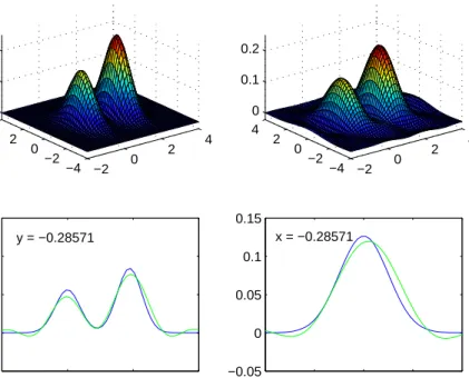
−2 0 2 4 −4 −2 0 2 4 0 0.1 0.2 −2 0 2 4 −4 −2 0 2 4 0 0.1 0.2 −2 0 2 4 −0.1 0 0.1 0.2 0.3 y = −0.28571 −4 −2 0 2 4 −0.05 0 0.05 0.1 0.15 x = −0.28571
Figure 1. Example 2, global bandwidth selection, with n = 500. Top right: true density f, top left: estimator fˇ, bottom: sections, dark line for f and light line for the estimator
withDh= [−1/h1,1/h1]×[−1/h2,1/h2]. Then, if Dh′′⊂Dh′, kfˆh′ −fˆh′′k2 = 1 4π2 Z Dh′\Dh′′ c f∗ Y f∗ ε 2 = 1 4π2 Z Dh′ c f∗ Y f∗ ε 2 − 1 4π2 Z Dh′′ c f∗ Y f∗ ε 2 =kfˆh′k2− kfˆh′′k2,
where we havekfˆhk2 =Pj|ˆahj|2. Then the computation of
A(h) = sup h′∈H q kfˆh′k2− kfˆh∨h′k2− q ˜ V(h′) +
is considerably accelerated. We choose V˜(h) = 0.05 log2(n)V(h), that isC(h)in formula (19) is taken equal to log2(n) as recommended by Corollary 3. Once the bandwidth is selected in the global setting, we have the coefficients ˆahjˆ and thus, we can plotfˆˆh(x, y) at any point (x, y).
We takeH andH0 included in{4/m,1 ≤m≤3n1/4}.
5.2. Examples. Now we compute estimators for different signal densities and different noises. Letλ= 6,µ= 1/4.
Example 1 Cauchy distribution: f(x, y) = (π2(1 +x2)(1 +y2))−1 on[−4,4]2 with a Laplace/Laplace
noise, i.e. fε(x, y) = λ2 4 e −λ|x|e−λ|y|; f∗ ε(x, y) = λ2 λ2+x2 λ2 λ2+y2
The smoothness parameters are b1 =b2= 0,r1=r2= 1,β1 =β2 = 2and ρ1 =ρ2 = 0.
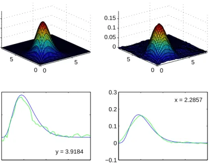
0 5 0 5 0 0.05 0.1 0.15 0 5 0 5 0 0.05 0.1 0.15 0 2 4 6 8 −0.02 0 0.02 0.04 y = 3.9184 0 2 4 6 8 −0.1 0 0.1 0.2 0.3 x = 2.2857
Figure 2. Example 3, pointwise bandwidth selection,with n= 500. Top right: true density f, top left: estimator f˜, bottom: sections, dark line for f and light line for the estimator
Example 2 Mixed Gaussian distribution: Xi,1=W/
√
7withW ∼0.4N(0,1) + 0.6N(5,1), and Xi,2
independent with distributionN(0,1). We estimate the density on[−2,4]2. We consider that the noise follows a Laplace/Gaussian distribution, i.e.
fε(x, y) = λ 2e −λ|x| 1 µ√2πe −y2/(2µ2) ; fε∗(x, y) = λ 2 λ2+x2e− µ2y2/2
The smoothness parameters are b1 = b2 = 0, r1 = r2 = 2, β1 = 2, β2 = 0 and
ρ1 = 0, α2 = µ2/2, ρ2 = 2. Here the rate of convergence is n−16/17[log(n)]63/34 in
the global setting and n−16/17[log(n)]23/17 for the bandwidths h−11 = p7 log(n) and
h−21=palog(n)−blog(log(n))fora= 16/17 andb= 40/17in both cases. We use that
µ2 = 1/16. n= 100 n= 300 n= 500 n= 750 n= 1000 Ex 1 Global 0.419 0.289 0.215 0.161 0.137 Ex 1 Pointwise 0.269 0.140 0.101 0.083 0.068 Ex 2 Global 3.615 1.699 0.761 0.473 0.367 Ex 2 Pointwise 3.477 1.714 0.799 0.526 0.363 Ex 3 Global 0.800 0.402 0.303 0.248 0.212 Ex 3 Pointwise 0.622 0.293 0.212 0.167 0.138
Example 3 Gamma distribution: Xi,1 ∼Γ(5,1/
√
5)andXi,2∼Γ(5,1/
√
5). We estimate the density on [0,8]2. The noise follow a Gaussian/Gaussian distribution, i.e.
fε(x, y) = 1
2πµ2e−
(x2+y2)/(2µ2)
; fε∗(x, y) =e−µ2(x2+y2)/2
So b1 =b2 = 5, r1 =r2 = 0, β1 =β2 = 0, α1 = α2 = µ2/2 and ρ1 = ρ2 = 2. This is
an example with pointwise rate [log(n)]−4 and global rate (log(n))−9/2 (which is not so
slow, for instance, for n= 1000, this term is smaller than 1/n).
n= 100 n= 300 n= 500 n= 750 n= 1000
Ex 1 1.48 2.04 2.01 1.96 1.97
Ex 2 1.08 1.03 1.05 1.07 1.25
Ex 3 1.36 1.53 1.57 1.57 1.62
Table 2. Coracle averaged over 100 samples
For these examples, we apply both global and pointwise estimation procedure, and we compute the Mean Integrated Squared Error on a grid of 50×50 points. The MISE (multiplied by 100, averaged over 100 samples) is given in Table 1. For each path, we also compare the MISE for the global procedure with the minimum risk for all bandwidths of the collection. Table 2 gives the empirical version of the oracle constant defined by
Coracle=E k ˇ f −fk2 infh∈Hkfˆh−fk2 ! .
It shows that the adaptation is performing, since the risk for the chosen ˆh is very close to the best possible in the collection (the nearest of oneCoracle, the better the algorithm).
We also illustrate the results with some figures. Figure 1 shows the surface z = f(x, y) for Example 2 and the estimated surface z = ˇf(x, y) obtained by global bandwidth selection. For more visibility, sections of the previous surface are drawn. We can see the curvesz=f(x,−0.3)
versus z = ˇf(x,−0.3) and the curvesz =f(−0.3, y) versus z = ˇf(−0.3, y). For this figure, the selected bandwidth ishˆ= (0.29,0.57). Thus, the bandwidth in the first direction is twice smaller, to recover the two modes: this shows that our procedure takes really anisotropy into account. Figure 2 is an analogous illustration of Example 3, but with a pointwise bandwidth selection, as described in Section 3. We obtain a slightly more angular figure. Nevertheless, we can notice by observing Table 1 that the MISE is almost always smaller for this kind of estimation.
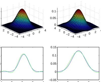
To conclude this section, we would like to mention that we can keep good results even in case of dependent components of both the noise and the signal. More precisely, we can take
X ∼ N(0,Σ) and ε∼ N(0,Σε) with Σ = 1 −0.7 −0.7 2 and Σε = 10−2 1 0.25 0.25 1.0625 ,
with X and ε independent. We present in Figure 3 an illustration of the results for the global method.
6. Concluding remarks: the case of unknown noise density
The assumption of the knowledge of the error distribution is often disputed. Relaxing this assumption requires conditions for obvious reasons of identifiability. Here is a quick description of what can be done in case of additional observations of the noise ε−1, . . . , ε−N (think of a
−4 −2 0 2 4 −4 −2 0 2 4 0 0.05 0.1 −4 −2 0 2 4 −4 −2 0 2 4 0 0.05 0.1 −4 −2 0 2 4 −0.05 0 0.05 0.1 0.15 −4 −2 0 2 4 −0.05 0 0.05 0.1 0.15
Figure 3. Dependent case, global bandwidth selection,withn= 500. Top right: true density f, top left: estimator f˜, bottom: sections, dark line for f and light line for the estimator
measure device calibrated without signal). We use this preliminary noise sample to estimatefε∗
in the following way
1 ˜ f∗ ε(x) = 1{|fˆε∗(x)|≥N−1/2} ˆ fε∗(x) = 1 ˆ fε∗(x) if | ˆ f∗ ε(x)| ≥N−1/2, 0 otherwise, where fˆ∗ ε(x) =N−1 PN
j=1e−ihx,ε−ji is the natural estimator offε∗. Then it is sufficient to write
¯
fh∗(t) =Kh∗(t)fcY∗(t) ˜
f∗
ε(t)
to define new estimators off in this context. Adapting all the previous results in this framework is beyond the scope of this paper, but we can observe the effect of this modification on the integrated squared error, for instance. The bias is unchanged, but an additional term appears in the variance:
Proposition 5. We have Ekfh−f¯hk2 .V(h) +W(h) where
W(h) = 1 (2π)dN Kh∗f∗ fε∗ 2 .
It is possible to give a bound of W(h) in term of the smoothness indices of fε and f but
we skip this tedious formula, which is just a generalization of Lemma 2 in Comte and Lacour [2011]. In the case of an ordinary smooth function and a fully ordinary smooth noise, we obtain
W(h).N−1Qdj=1h−2(βj−bj)+
Thus, we get new rates of convergence in terms of n and N. If N > n, W(h) is always smaller thanV(h). In this case, an adaptive procedure is conceivable, replacingV˜(h) byV¯(h) =
¯ C(h) Kh∗/f˜ε∗
2/n and modifying H in the same way. The efficiency of this strategy can be proved by controlling terms of the form [kf¯h−fˆhk2−V¯(h)]+. This was successfully established
in Comte and Lacour [2011] in dimension 1, but such a study in dimensiondwould be much too long here.
7. Proofs
We start with three useful lemmas.
Lemma 1. Consider c, s nonnegative real numbers, and γ a real such that 2γ >−1 ifc= 0 or
s= 0. Then, for all m >0,
• R−mm(x2+ 1)γexp(c|x|js)dx≈m2γ+1−secm s , and if in addition 2γ >1 if c= 0 or s= 0, • Rm∞(x2+ 1)−γexp(−c|x|s)dx≈m−2γ+1−se−cm s .
Proof of this lemma is based on integration by parts and is omitted. See also Lemma 2 p. 35 in Butucea and Tsybakov [2008a].
Lemma 2. [Bernstein inequality] Let T1, . . . , Tn be independent random variables and Sn(T) =
Pn i=1[Ti−E(Ti)]. Then, for η >0, P(|Sn(T)−E(Sn(T))| ≥nη) ≤ 2 max exp −nη 2 4v ,exp−nη 4b ,
where Var(T1)≤v and|T1| ≤b.
It is proved in Birgé and Massart [1998], p.366 that P(|Sn(T)−E(Sn(T))| ≥nη)≤
2 exp −nη2/(2v2+ 2bη). Lemma 2 follows.
Lemma 3. [Talagrand Inequality] LetY1, . . . , Ynbe i.i.d. random variables andνn(t) = n1 Pni=1|ψt(Yi)−
E(ψt(Yi))] for t belonging to B¯ a countable subset of functions. For any η >0,
(27) P(sup t∈B¯ |νn(t)| ≥(1 + 2η)H)≤max exp −η 2 6 nH2 v ,exp −min(η,1)η 21 nH M . and (28) E h sup t∈B¯ |νn(t)| −(1 + 2η)H i + ≤ r 3π 2 r v ne −η62nH 2 v + 21 η∧1 M ne −(η∧211)ηnHM , with sup t∈B¯k ψtk∞≤M, E h sup t∈B¯| νn(t)| i ≤H, sup t∈B¯ 1 n n X k=1 Var(ψt(Yk))≤v.
Proof of Lemma 3: We apply the Talagrand concentration inequality given in Klein and Rio [2005] to the functionssi(x) =t(x)−E(t(Y i))and we obtain P(sup t∈B¯| νn(t)| ≥H+λ)≤exp − nλ 2 2(v+ 4HM) + 6M λ .
Then we modify this inequality following Birgé and Massart [1998] Corollary 2 p.354. It gives
(29) P(sup t∈B¯| νn(t)| ≥(1 +η)H+λ)≤exp −n3min λ2 2v, min(η,1)λ 7M .
To conclude for (27), we setλ=ηH. For (28), we takeλ=ηH+u and write
Eh sup t∈B¯(0,1) |νn(t)| −(1 + 2η)H i + ≤ Z +∞ 0 P sup t∈B¯(0,1) |νn(t)| ≥(1 +η)H+ηH+u ! du ≤ Z +∞ 0 e−nη 2H2 6v e−nu 2 6v du+ Z +∞ 0 e−nη(η21M∧1)He− n(η∧1)u 21M du = r 3π 2 r v ne− nη2H2 6v + 21M n(η∧1)e− nη(η∧1)H 21M
which is the result of (28).
7.1. Proof of Proposition 1. In the first case, the bias term is the same as in density esti-mation (see Tsybakov [2009]) and the use of Taylor formula to partial functions t 7→ f(x1 −
v1h1, . . . , xi−1−vi−1hi−1, t, xi+1, . . . , xd)yield |fh(x0)−f(x0)| ≤L d X j=1 R |xj|bj|K(x)|dx ⌊bj⌋! hbj j .
In the second case, since f∗, fh∗∈L1(R), we can write
f(x0)−fh(x0) = 1 (2π)d Z e−ihx0,ui1 (Qdj=1[−1/hj,1/hj])c(uj)f ∗(u 1, . . . , ud)du1. . . dud
Then, for f ∈ S(b, a, r, L), the bias term is
|f(x0)−fh(x0)| ≤ 1 (2π)d d X j=1 Z 1|uj|≥1/hj|f∗(u1, . . . , ud)|du1. . . dud ≤ (2π1)d d X j=1 Z " 1|uj|≥1/hj| d Y k=1 (1 +u2k)−bk/2exp(−a k|uk|rk) # × " |f∗(u1, . . . , ud)| d Y k=1 (1 +u2k)bk/2exp(a k|uk|rk) # du1. . . dud ≤ (2Lπ)d d X j=1 Z |u|≥1/hj (1 +u2)−bjexp(−2a j|u|rj)du !1/2 since Y k6=j (1 +u2k)−bk/2exp(−a k|uk|rk)≤1.
Then, using Lemma 1, |f(x0)−fh(x0)|.LPdj=1h
bj+rj/2−1/2
j exp(−ajh−jr).
7.2. Proof of Proposition 2. The independence of the observations gives
Var( ˆfh(x0)) = 1 nVar 1 (2π)d Z e−ihu,x0iK∗ h(u) eihu,Y1i fε∗(u) du ! .
A simple bound of the variance by the expectation of the square yieldsVar( ˆfh(x0))≤(n(2π)2d)−1kKh∗/fε∗k21.
But we can also write
Var( ˆfh(x0))n(2π)2d = Z Z e−ihu−v,x0iK ∗ h(u)Kh∗(−v) f∗ ε(u)fε∗(−v) (fY∗(u−v)−fY∗(u)fY∗(−v))dudv ≤ Z Z Kh∗(u)Kh∗(−v) f∗ ε(u)fε∗(−v) |fY∗(u−v)|dudv ≤ Z Kf∗h∗(u) ε(u) 2 du Z |fY∗(t)|dt≤ Kh∗ f∗ ε 2 2 kfε∗k1
using Schwarz inequality.
Now, under (Hε),(2π)2dnV0(h) is bounded by the minimum of
kfε∗k1 d Y j=1 Z Kj∗(ujhj) (u2j + 1)−βj/2exp(−α j|uj|ρj) 2 duj and d Y j=1 Z K∗ j(ujhj) (u2 j + 1)−βj/2exp(−αj|uj|ρj) duj 2 .
Ifj∈SS, i.e. ρj >0thenKj∗(t) = 0 if |t| ≥1. Consequently, using Lemma 1,
Z Kj∗(uhj) (u2+ 1)−βj/2exp(−α j|u|ρj) 2 du = Z 1/hj −1/hj |Kj∗(uh)|2(u2+ 1)βjexp(2α j|u|ρj)du ≤ kKj∗k2∞ Z 1/hj −1/hj (u2+ 1)βjexp(2α j|u|ρj)du . h−2βj−1+ρj j exp(2αjh −ρj j ).
In the same way
Z Kj∗(uhj) (u2+ 1)−βj/2exp(−α j|u|ρj) du = Z 1/hj −1/hj |Kj∗(uh)|(u2+ 1)βj/2exp(α j|u|ρj)du ≤ kKj∗k∞ Z 1/hj −1/hj (u2+ 1)βj/2exp(α j|u|ρj)du . h−βj−1+ρj j exp(αjh−jρj).
Now, ifj ∈OS, i.e. αj =ρj = 0, then
Z Kj∗(uhj) (u2+ 1)−βj/2 2 du=h−j1 Z |Kj∗(u)|2((uh−j1)2+ 1)βjdu.h−1−2βj j Z |Kj∗(u)|2(u2+ 1)βjdu and Z K ∗ j(uhj) (u2+ 1)−βj/2 du . h−j1−βj Z
|Kj∗(u)|(u2 + 1)βj/2du. Finally, using that h
j ≤ 1, we
obtain the following bound fornV0(h)
Y j∈SS min(1, h−1+ρj j )h −2βj−1+ρj j exp(2αjh −ρj j ) Y j∈0S h−1−2βj j = d Y j=1 h(ρj−1)+ j h −2βj−1+ρj j exp(2αjh −ρj j ).
7.3. Proof of Theorem 1. We shall consider two cases:
• Case A: the noise is OS and f belongs to D= H(b, L) or D =S(b+ 1/2, a, r, L), with
0≤rj <2 for allj= 1, . . . , d.
In this case we set hn such that hn,j = n−1/(2bj+bj
Pj0
i=1[(2βi+1)/bi]) if r
j = 0 (ordinary
smooth components of f) and hn,j = (log(n)/(2aj))−1/rj when rj > 0 (super smooth
components). Moreover ψn is defined by (10) (recall that we standardized notations by
setting rj = 0 when Hölder smoothness is considered, thus in the case of none super
smooth components, we retrieve optimal hn given by (5) and rate (6)).
• Case B: the noise has at least one SS component and f belongs to D = H(b, L) or
D=S(b+ 1/2,0,0, L).
Then we sethn,j =n−1/(2βj+2bj+1)forj ∈OS, and forj∈SS,hn,j = (2ρjlog(n)/αj)−1/ρj.
We recall that in this case ψn= [log(n)]−2 minj∈SS(bj/ρj).
Before starting with the proof, we need to define preliminary material.
Let H be the kernel function defined in Fan [1991], which is such that: R H = 0, H(0)6= 0,
H ∈ H(bi, L)∩ S(bi,0,0, L), for i = 1, . . . , d, |H(x)| = O(x−δ) as |x| → ∞ with δ > 3, and
H∗(t) = 0, (and thus also(H∗)′(t) = 0, (H∗)′′(t) = 0) when |t|is outside [1,2].
We also usegsthe symmetric stable law with characteristic functiongs∗(u) = exp(−|u|s)where
0< s <2. An interest of this function relies on the Lemma:
Lemma 4. The density gs satisfies the following properties:
• gs−1(x) =O(|x|s+1)
• Ifs <1, for allb >0, there existsL′ such thatgsbelongs to the Hölder space of dimension
one H(b, L′).
Proof of Lemma 4: Since the density is symmetric, we only consider positive x. Devroye [1986] shows that, forx >0,gs(x) =x−1P∞j=1bj(x−s)j with
bj =
(−1)j−1Γ(sj+ 1) sin(sjπ/2)
πj!
First, we can write
gs(x) =b1x−s−1+o(x−s−1)
asx→ ∞, which proves the first point for s <1. The cases≥1can be found in Butucea and Tsybakov [2008b]. The power series Pbjuj converges for all x (as pointed by Devroye, Stirling
formula allows to show a geometric convergence –in fact of order jj(s−1)). So it is differentiable with differentiatePjbjuj−1. Then, an easy computation leads to
gs′(x) = ∞
X
j=1
bj(−1−sj)x−sj−2=b1(−1−s)x−s−2+o(x−s−2)
in some neighbourhood of infinity. In the same way, for allk≥0,
g(sk+1)(x) =cx−s−k−2+o(x−s−k−2).
But Hölder inequality provides |gs(k)(x′) −gs(k)(x)| ≤ (R|g(sk+1)|p)1/p|x −x′|b−k where 1/p =
1 +k−b. Since s+k+ 2> k+ 1−b,p(s+k+ 2)>1 and gs(k+1) is in Lp. Thusgs∈ H(b, L′)
Now, we define two couples (f0, f1,A) and (f0, f1,B). From now on, we assume that x0 =
(0, . . . ,0) since it is sufficient to translate functions at point x0 in the other cases.
Case A. Let f0(x) = d Y j=1 1 cj gsj xj cj
with cj positive constants large enough (they will be made precise later). Heresj = s <1 for
j = 1, . . . , d if D = H(b, L), and if D = S(b+ 1/2, a, r, L), for rj < 1, rj < sj < 1 and for
1≤rj <2,rj < sj <2. We also define f1,A(x) =f0(x) +c p V0(hn) d Y j=1 H xj 2hn,j . Case B. Here we considerf0 withsj =s <1 for allj, and
f1,B(x) =f0(x) +c d X j=1 hbj n,jH xj hn,j Y 1≤i≤d, i6=j gs(xi),
where c is a constant to be specified later. In the sequel we show that, for Z =A, B,
1) f0 andf1,Z are density functions and belong to D.
2) χ2(Pfn1,Z, Pfn0) . n−1 where Pfn1,Z (resp. Pfn0) is the probability associated with the distribution of a sampleY1, . . . , Ynfor density ofY1given byf1,Z(respf0) andχ2(P, Q) =
R
(dP/dQ−1)2dQ. 3) |f1,Z(x0)−f0(x0)| ≥Cψn.
Then it is sufficient to use Theorem 2.2 (see also p.80) in Tsybakov [2009] to obtain Theorem 1. Proof of 1).
Hypothesis functions are densities
First,f0are densities by construction. Second, the definition ofHguarantees that, forZ =A, B,
R
f1,Z = 1. To ensure the positivity off1,Z, it is sufficient to prove that|f1,Z−f0| ≤f0. But, as
|x| → ∞, f0−1(x)|f1,A(x)−f0(x)|.c p V0(hn) d Y j=1 hδn,j d Y j=1 xsj+1−δ j ≤1
for csmall enough, since δ >3>max(sj) + 1. In the same way, for case B, as |x| → ∞,
f0−1(x)|f1,B(x)−f0(x)|.c d X j=1 hbj+δ n,j x sj+1−δ j ≤1
for csmall enough.
Belonging to the Hölder space
Recall that we take s <1 when D is an Hölder space. Since gs is in Hölder space of dimension
one for any smoothness (Lemma 4),f0∈ H(b, L′)for someL′, and it is sufficient to choosecj to
Now letGA(.) = (f1,A−f0)(x1, . . . , xj−1, . , xj+1, . . . , xd). SinceH∈ H(bj, L), |G(Ak)(x′)−GA(k)(x)| = cpV0(hn) Y j6=i H xj 2hn,j (2hn,i)−k H(k) x′ 2hn,i −H(k) x 2hn,i ≤ ckHk∞d−1LpV0(hn)(2hn,i)−bi|x′−x|bi−k. Then f1,A−f0 ∈ H(b, L/2) as soon as ckHkd∞−1 p
V0(hn)(2hn,i)−bi ≤ 1/2, which holds for our
selected hn and suitablec. Thus f0 andf1,A belong to H(b, L).
Now letGB(.) = (f1,B−f0)(x1, . . . , xj−1, . , xj+1, . . . , xd). SinceH ∈ H(bj, L),
|G(Bk)(x′)−G(Bk)(x)| ≤ chbj n,jh−n,jk H(k) x′ hn,j −H(k) xj hn,j kgskd∞−1 +cLkgskd∞−2kHk∞ X p6=j hbp n,p|x−x′|bj−k ≤ chbj n,jh−n,jkL x−x′ hn,j bj−k kgskd∞−1+cdLkgsk∞d−2kHk∞|x−x′|bj−k
Thenf1,B−f0 ∈ H(b, L/2) if c is chosen small enough, so that f1,B belongs toH(b, L). Belonging to the Sobolev space
By construction and because sj > rj, for cj large enough, f0 ∈ S(b+ 1/2, a, r, L/2) for rj <2,
j= 1, . . . , d. The computation of the Fourier transform of f1,A−f0 gives
|(f1,A−f0)∗(t)|=c p V0(hn) d Y j=1 2hn,j|H∗(2tjhn,j)|. Therefore Z |(f1,A−f0)∗(t)|2 d X j=1 (1 +t2j)bj+1/2exp(2a j|tj|rj)dt ≤ c2V0(hn) d X j=1 h2n,j Z |H∗(2tjhn,j)|2(1 +t2j)bj+1/2exp(2aj|tj|rj)dtj Y k6=j hn,k Z |H∗(2tkhn,k)|2dtk ≤ C(H)c2V0(hn) d X j=1 h−2bj n,j exp(2ajh− rj n,j ),
using that H∗(t) = 0 when |t| is outside [1,2]. Then f1,A−f0 ∈ S(b+ 1/2, a, r, L/2) as soon
as C(H)c2V
0(hn)h−n,i2biexp(2aihn,i−ri) ≤ L2/(4d). This is verified for hn as chosen (the variance
dominates the bias).
The computation of the Fourier transform off1,B−f0 gives
(f1,B−f0)∗(t) =c d X k=1 hbk+1 n,k H∗(tkhn,k) d Y ℓ=1,ℓ6=k gs∗(tℓ).
Therefore d X j=1 Z |(f1,B−f0)∗(t)|2(1 +t2j)bj+1/2dt ≤ c2d d X j=1 h2bj+2 n,j Z |H∗(tjhn,j)|2(1 +t2j)bj+1/2dtj d Y i=1,i6=j Z |gs∗(ti)|2dti +c2d X 1≤j,k≤d,j6=k h2bk+2 n,k Z |H∗(tkhn,k)|2dtk Z (1 +t2j)bj+1/2|g∗ s(tj)|2dtj Y ℓ6=k, ℓ6=j Z |gs∗(tℓ)|2dtℓ
which is bounded sinceR |H∗(tjhn,j)|2(1 +t2
j)bj+1/2dtj =O(h−n,j2bj−2),R(1 +t2j)bj+1/2|g∗s(tj)|2dtj
is a finite constant andh2bk+2
n,k
R |g∗
s(tkhn,k)|2dtk =O(h2n,kbk+1) =o(1). Then there is somecsuch
thatf1,B−f0 ∈ S(b+ 1/2,0,0, L/2).
Proof of 2). Chi-square divergence
ForZ=A, B, since the observations are i.i.d.,χ2(Pfn1,Z, Pfn0) = (1 +χ2(Pf1,Z, Pf0))
n−1(see e.g.
Tsybakov [2009] p.86). Thus, it is sufficient to prove that χ2(Pf1,Z, Pf0) =O(n−
1) where
χ2(Pf1,Z, Pf0) = Z
(f1,Z∗fε−f0∗fε)2(f0∗fε)−1.
Recall that we assume the independence of the noise components. Let us denote
qj(xj) = Z 1 cj gsj xj −y cj fε1,j(y)dy= 1 cj gsj . cj ∗fε1,j(xj) so thatQjqj(xj) = (f0∗fε)(x). Then χ2(Pf1,A, Pf0) = c 2V 0(hn) d Y j=1 Z Z H xj−y 2hn,j fε1,j(y)dy 2 q−j1(xj)dxj and χ2(Pf1,B, Pf0) ≤ c 2d d X j=1 h2bj n,j Z Z H xj−y hn,j fε1,j(y)dy 2 q−j1(xj)dxj ×Y j6=i Z qi(x)dx and Z qi(x)dx= 1,
Now it follows from our Lemma 4 and Fan [1991]’s Lemma 5.1 that qj(xj) ≥ C|xj|−(sj+1) for
|xj| large enough, say |xj| ≥ A ≥1. Indeed Fan [1991]’s proof of his Lemma 5.1 works in our
case because of the heavy tail property in Lemma 4. Using this property, we prove that
Z Z H xj−y hn,j fε1,j(y)dy 2 qj−1(xj)dxj =O(hn,j2βj+1exp(−21−ρjαjh−n,jρj)). (30)