Southern Methodist University Southern Methodist University
SMU Scholar
SMU Scholar
Engineering Management, Information, and
Systems Research Theses and Dissertations Engineering Management, Information, and Systems
Spring 5-16-2020
A Data-Driven Framework for Decision Making Under Uncertainty:
A Data-Driven Framework for Decision Making Under Uncertainty:
Integrating Markov Decision Processes, Hidden Markov Models
Integrating Markov Decision Processes, Hidden Markov Models
and Predictive Modeling
and Predictive Modeling
Hossein Kamalzadeh
Southern Methodist University, [email protected]
Follow this and additional works at: https://scholar.smu.edu/engineering_managment_etds
Part of the Operational Research Commons, and the Other Operations Research, Systems Engineering and Industrial Engineering Commons
Recommended Citation Recommended Citation
Kamalzadeh, Hossein, "A Data-Driven Framework for Decision Making Under Uncertainty: Integrating Markov Decision Processes, Hidden Markov Models and Predictive Modeling" (2020). Engineering Management, Information, and Systems Research Theses and Dissertations. 11.
https://scholar.smu.edu/engineering_managment_etds/11
This Dissertation is brought to you for free and open access by the Engineering Management, Information, and Systems at SMU Scholar. It has been accepted for inclusion in Engineering Management, Information, and Systems Research Theses and Dissertations by an authorized administrator of SMU Scholar. For more information, please visit http://digitalrepository.smu.edu.
A DATA-DRIVEN FRAMEWORK FOR DECISION MAKING UNDER UNCERTAINTY:
INTEGRATING MARKOV DECISION PROCESSES, HIDDEN MARKOV MODELS AND PREDICTIVE MODELING
Approved by: Dr. Michael Hahsler Dr. Eli Olinick Dr. Halit Uster Dr. Aurelie Thiele Dr. Vishal Ahuja Dr. Jay Rosenberger
A DATA-DRIVEN FRAMEWORK FOR DECISION MAKING UNDER UNCERTAINTY:
INTEGRATING MARKOV DECISION PROCESSES, HIDDEN MARKOV MODELS AND PREDICTIVE MODELING
A Ph.D. Dissertation Presented to the Graduate Faculty of the
Lyle School of Engineering: Engineering Management, Information, and Systems Southern Methodist University
in
Partial Fulfillment of the Requirements for the degree of
Doctor of Philosophy with a
Major in Operations Research by
Hossein Kamalzadeh
(B.S., Isfahan University of Technology, 2014) (M.S., Amirkabir University of Technology, 2016)
Kamalzadeh, Hossein B.S., Isfahan University of Technology, 2014 M.S., Amirkabir University of Technology, 2016 A Data-Driven Framework for Decision Making Under Uncertainty:
Integrating Markov Decision Processes, Hidden Markov Models and Predictive Modeling
Advisor: Professor Michael Hahsler
Doctor of Philosophy conferred May, 16, 2020 Dissertation completed Jan, 20, 2020
The problem of decision making under uncertainty can be broken down into two parts. First, how do we learn about the world? This involves the problem of modeling the system and its uncertainty. Secondly, given what we currently know about the world, how should we decide what to do, taking into account uncertainty of future events and observations that may change our conclusions. Many systems evolve over time and often the next state of the system is not known with certainty, often modeled as a probability distribution over system states. Dealing with such systems especially when we can make a decision at different points in time is difficult due to uncertainty. Making optimal decisions requires understanding the system including its characteristics, how it evolves and changes over time, and how taken actions affect the system. There are multiple dimensions to this problem, and each dimension might require its own specific method. We need a descriptive method that can summarize the system and its evolution, a predictive model that is used to extract information from the complicated systems and also a prescriptive model that works as the main decision model and incorporates the effects of actions. In this thesis I consider Partially Observable Markov Decision Process (POMDP) as the main decision-making/prescriptive model, Hidden Markov Models (HMM) as the descriptive model of system evolution, and a predictive model to create observations
for the POMDP. In this research, I develop a framework by combining these methods and demonstrate its use with two applications. I apply the proposed framework to the problem of diabetes screening and also resource allocation under uncertainty for emergency management. I demonstrate using simulation that implementing the proposed policy will bring about significant improvements in both systems compared to the existing policies.
Keywords: decision-making under uncertainty, predictive analytics, Markov
TABLE OF CONTENTS
CHAPTER
1.
Introduction
. . . 11.1. Contributions . . . 2
1.2. Methodology . . . 2
1.3. Motivations and Applications . . . 3
1.4. Structure of this thesis . . . 5
2.
A Data-Driven Decision Framework
. . . 72.1. Stochastic systems and their evolution . . . 8
2.2. Introduction to Partially Observable Markov Decision Processes . . . 10
2.3. Literature related to Partially Observable Markov Decision Processes . . . 13
2.4. Predictive Modeling for Observation Aggregation . . . 14
3.
Optimal Individualized Diabetes Screening (P1)
. . . 183.1. Background on Diabetes . . . 18
3.2. Related Literature . . . 20
3.2.1. MDP for Medical Decision Making . . . 21
3.2.2. HMM to Model Disease Progression . . . 22
3.2.3. Predictive Models in Healthcare . . . 23
3.3. The Partially Observable Markov Decision Process Formulation . . . 24
3.3.1. Time Horizon and Decision Epochs . . . 25
3.3.2. State Space . . . 25
3.3.3. Action Space . . . 25
3.3.4. Transition Probabilities . . . 25
3.3.5. Observations and Observation Probabilities . . . 27
3.3.6. Belief States . . . 27
3.3.7. Reward Functions . . . 28
3.3.8. Bayesian Belief State Update and Optimality Equation . . . 28
3.4. Hidden Markov Models . . . 29
3.5. The Predictive Risk Model . . . 31
3.6. Parameter Estimation . . . 32
3.6.1. Data Description . . . 32
3.6.2. Estimating Transition Probabilities . . . 33
3.6.3. Estimating Observation Probabilities . . . 35
3.6.4. Estimating Rewards . . . 36
3.8. Policy Implications And Evaluations . . . 41
3.8.1. Simulation Model for Guidelines Evaluation . . . 41
3.8.2. Guidelines Evaluation . . . 42
3.8.3. Sensitivity Analysis of the Simulation Model . . . 44
4.
Resource Allocation Under Uncertainty for Emergency
Situations (P2)
. . . 484.1. The need for a resource reallocation policy . . . 48
4.2. The Partially Observable Markov Decision Process Formulation . . . 51
4.2.1. State Space . . . 51 4.2.2. Action Space . . . 52 4.2.3. Observations . . . 53 4.2.4. Cost Structure . . . 53 4.3. Parameter Estimation . . . 53 4.3.1. Data Description . . . 53
4.3.2. Estimating Transition Probabilities . . . 55
4.3.3. Estimating observation probabilities . . . 57
4.3.4. Costs . . . 59
4.4. Optimal Reallocation Policy . . . 62
4.5. Policy Evaluation using Simulation . . . 62
4.5.1. Simulation parameter estimation . . . 63
4.5.2. Evaluation using simulation . . . 68
5.
Conclusion
. . . 705.1. Optimal Individualized Diabetes Screening . . . 71
5.2. Resource Allocation Under Uncertainty for Emergency Vehicles . . . 73
APPENDIX A. Diabetes Simulation Details . . . 75
A.1. Patient Instantiation . . . 75
A.2. Updating Health Status . . . 76
A.3. Calculating Patient’s Utility . . . 76
A.4. Check for Diagnosis . . . 76
A.5. Patient’s Annual Costs . . . 79
A.6. Leaving the Simulation . . . 79
A.7. Implementing POMDP Policy/Other Guidelines . . . 80
List of Tables
3.1 Key characteristics of the cohort studied . . . 33
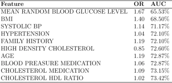
3.2 Top 10 features of the proposed regularized multinominal regression model . . . 36
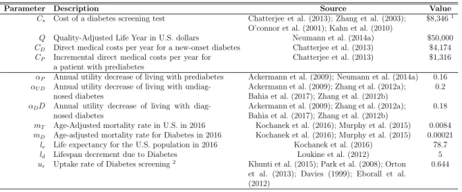
3.3 Parameters associated with the reward function of the POMDP model . . . 37
3.4 comparison between various screening guidelines in terms of cost-effectiveness, years and QALYs gained, diagnosis lead time and events prevented (from 50 replications) . . . 43
3.5 Sensitivity analysis for varying each paramter by +/-20% . . . 46
4.1 Dispatches from other zones to zone 1 from 2015 to 2017 . . . 49
4.2 POMDP model state space and dimensions . . . 52
4.3 Basic information on the data provided by the DFRD . . . 56
4.4 Transition probabilities for actionaask. . . 59
4.5 Transition probabilities for actionanothing . . . 59
4.6 Observation probabilities (confusion matrix) from the predictive model . . . 60
4.7 Action and state dependent costs of the POMDP model (in minutes) . . . 61
4.8 Optimal reallocation policy produced by POMDP . . . 63
4.9 Distribution fitting analysis for incidents inter-arrival times . . . 64
4.10 Distribution fitting analysis for response times . . . 65
4.11 Incident types and their respective probabilities of happening . . . 66
4.12 Comparison of two scenarios in various metrics . . . 69
A.1 Prevalence rates of Diabetes and its complications stages . . . 77
A.2 Progression rates for transitions in Diabetes and its complications . . . 77
A.3 Life utilities for different health conditions . . . 79
Chapter 1
Introduction
The problem of decision making under uncertainty can be broken down into two parts. First, how do we learn about the world? This involves both the problem of modeling our uncertainty about the world, and that of drawing conclusions from evidence and our initial information. Secondly, given what we currently know about the world, how should we decide what to do, taking into account future events and observations that may change our conclusions (Dimitrakakis and Ortner (2018)). In other words, understanding the system for which we are trying to make a decision plays an important role in making an optimal decision at any point in time. This understanding includes knowledge about the currently most likely state of the system, and how it may evolve over time. The next step is to find a method to make optimal decision.
Many systems evolve over time in a discrete manner where their status changes from one state to another. Often, the state of the system is not known with certainty. Dealing with such systems especially when we have to make a decision at some point in time is difficult due to our uncertainty about the system. Though the short term effects of the decision made now might be obvious to the decision maker, the long term consequences of such decisions are hard to estimate since the system has inherent uncertainty associated with it. In other words, the decision maker might think that the decision he is making right now is the best since it seems to have the largest short-term reward, the long-term effects on the system are less certain. This can be more complicated if the decisions can affect how the system changes from one state to another. An example is called the tiger problem (Cassandra et al. (1994)), where you are trapped in a room with two doors. Behind one of the doors is a hungry tiger waiting to eat you while behind the other is a treasure. You have no idea behind which door the tiger is. You can open either doors or listen to see if you can hear anything. Listening is
not accurate since you might hear the tiger behind the left door while it is actually behind the right one. Making the optimal decision (how long to listen before opening a door) in such a system demands understanding the uncertainty, and how the actions taken reduce uncertainty.
1.1. Contributions
Making optimal decisions under uncertainty, requires understanding the system including its characteristics, how it evolves and changes, and how the actions affect the system over time. This demands special tools and methods to deal with, and it might also require integration of multiple methods from different areas; methods that help us model the underlying states of a system, and how these states evolve into each other. A descriptive method handles modeling the system and its evolution. A prescriptive model works as the main decision model and analyses the effects of actions and decisions on the system and in long term. A predictive model is used to extract information from the system, providing the decision model with information that the actual descriptive model may not be able to provide. The major contribution of this research is the integration of these methods in a single data-driven framework and the application to several problems. An R package named ’pomdp’ is also developed to support this research, enabling the user to easily define POMDP models and solve them. The manual of the package can be found in the appendix.
1.2. Methodology
The main problem this research is dealing with is the difficulty of making optimal decisions in situations that have inherent uncertainty stemming from a complex system. These systems can often be modeled as a combination of multiple states that transition into each other with certain probabilities. This requires methods that can model the progression of these systems and take into account their multi-state nature. We will later see that this is the main reason why we have chosen methods such as Partially Observable Markov Decision Process (POMDP) as the main decision model for this research. We will clarify on the methods and
techniques used in this research later in chapter 2 and discuss the relation between them. In this research we use real data collected in a quantitative approach from the application areas studied. The data collected is analyzed from various perspectives to estimate the characteristics of the associated system it was collected from and these characteristics are later used to simulate a duplicate of the system in order to further analyze it.
This research is mainly model-based driven by idealized model (which is usually denoted as axiomatic research). The primary concern here is to obtain optimal solutions within the defined model and make sure that these solutions provide insights into the structure of the problem. Typically, axiomatic research is normative, although descriptive research, aimed at understanding the process that has been modeled, is also present. Normative research is primarily interested in developing policies, strategies, and actions, to improve over the results available in the existing literature, to find an optimal solution for a newly defined problem, or to compare various strategies for addressing a specific problem. Although in the axiomatic domain, the discussion on methodology is largely absent, the operational research approach of this research consists of a number of phases including (1) conceptualization, (2) modeling, (3) model solving, and (4) implementation (Will M. Bertrand and Fransoo (2002)).
In the conceptualization phase, we develop a conceptual model of the problem and system being studied. We make decisions about the variables that need to be included in the model, and the scope of the problem and model to be addressed. In the next phase, we actually build the quantitative model, thus defining causal relationships between the variables. After this, the model solving process takes place, in which the mathematics usually play a dominant role. Finally the results of the model are implemented, after which a new cycle can start.
1.3. Motivations and Applications
In this research, we examine two systems each having their own characteristics and behavior while we are trying to provide policies for the decision makers of each system, policies that work optimally given the uncertainty in the systems. We use the proposed
framework we talked about in the previous section of this chapter for both applications and we demonstrate how this framework and the integration of the methods we use works for both applications in providing optimal policies for decision makers in systems that have inherent uncertainty. For the first system, we focus on chronic diseases such as HIV, Diabetes, and CKD, where modeling the initial uncertainty about what stage of the disease the patient is in and what decision should be taken with respect to the patient’s status taking into account the future events are the major problems. For the second system, we mainly focus on emergency management, where the uncertainty lies in which area of the city is in need of more resources in the near future. What is common among these two systems, is first, they are both systems that have states changing over time with uncertainty associated with them, and second, the actions and decisions of the decision maker affects the system and has long term effect on it. We also use the same framework we talked about to deal with each system.
Application 1: Diabetes Screening: In chapter 3, we focus on chronic diseases
specifically diabetes. Type 2 diabetes (which for the sake of simplicity we call diabetes here) is a major cause of morbidity and mortality worldwide. Diabetes is the 7th leading cause of death in the U.S. and causes macro-vascular complications, including heart attacks and strokes, and micro-vascular complications including retinopathy, nephropathy, and neuropathy (Petersen (2016)). The number of people who have Diabetes worldwide was estimated to be 221 million in 2010 and is expected to increase to 300 million by 2025 (Bjork (2001)) In the U.S. 9.4% of the population (30.3 million) have diabetes, 7.2 million of which are undiagnosed. An additional 33.9% of the population (84.1 million) have prediabetes of which almost 77 million are undiagnosed (CDCP (2017)). Consequently, diabetes is a major source of medical expenditures in the form of direct medical costs including hospital inpatient care (43% of the total direct medical expenditures), prescription medication to treat the complications caused by diabetes (18%), antidiabetic agents and diabetic supplies (12%), physician office visits (9%), and nursing/residential facility stays (8%) (Petersen (2016)). In
the U.S., estimates of direct costs were increasing from $176 billion in 2012 to $237 billion in 2017 (American Diabetes Association (2018)). Diabetes also imposes high indirect costs due to work-related absenteeism, reduced productivity at work and home, reduced labor force participation from chronic disability and premature mortality which increased from $69 billion in 2012 to $90 billion in 2017 (American Diabetes Association (2018); Bjork (2001); Petersen (2016)).
Application 2: Emergency Management: In chapter 4, we focus on emergency
management. According to Dallas Fire and Rescue Department, a structural fire incident needs resources from several fire stations around the city which are close to the incident location, each providing a specific type of vehicle. This means if more than a single structural fire incident happens in a small area of a city within a short period of time, no resources would be available to be dispatched to the incident. This can cause huge damages.
An important question for the Dallas Fire and Rescue Department is whether resources should be moved around in the city to cover areas where the resources are currently responding to an ongoing incidence. Every time an incident happens, resources in a particular zone of the city will be dispatched and become unavailable for several hours. If another incident happens in that zone during that time, resources from other areas of the city will need to respond which will increase response time. To mitigate such situations, we can temporarily reallocate resources.
1.4. Structure of this thesis
In chapter 2, we propose to utilize and combine three techniques and methods in a single framework to model each system using its key characteristics. In our framework we have a descriptive model that uses the characteristics of the system’s evolution to model its changes over time including the inherent uncertainty in the changes. This model is learned directly from the data available from each application area. We use a prescriptive decision model, to optimize the decisions and actions the decision maker can make taking into account each
action’s immediate and long term effects on the system. The decision model provides us with an optimal policy. Additional information (signals) are provided using the predictive model. The predictive model is also directly learned from the available data.
In chapter 3, we focus on chronic diseases specifically diabetes. We propose a targeted screening policy (equivalently, screening strategy) that uses all available information on individual patients to identify whom to screen (that is, which patients should receive the gold-standard test) and when to screen them; the policy is also age-specific. We develop and validate our model on a detailed and proprietary dataset – of over 12,000 patients over an 18-month period – from a large safety-net hospital and demonstrate, using a simulation analysis, that our proposed screening policy can improve patient outcomes.
In chapter 4, we focus on emergency management. We apply the proposed framework, and formulate the problem as a POMDP problem. We focus on one city zone in order to define our state space. We try to capture the availability of the resources in that zone in the near future; By implementing the proposed POMDP policy, and through simulation, we demonstrate that we can improve the average response time by a significant amount compared to existing policies.
Chapter 5 concludes this thesis. In the appendix of this thesis, details of the simulations conducted as well as the manual to the R package ’pomdp’ developed to support the research are included.
Chapter 2
A Data-Driven Decision Framework
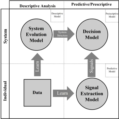
We propose to utilize and combine three techniques and methods in a single framework to create a decision framework that uses data in all main phases. In our framework we have a descriptive model that uses the characteristics of the system’s evolution to model its changes over time including the inherent uncertainty in the changes. This model is learned directly from the data available from each application area. We use a prescriptive decision model, to optimize the decisions and actions the decision maker can make taking into account each action’s immediate and long term effects on the system. The decision model provides us with an optimal policy. Additional information (signals) are provided using the predictive model. The predictive model is also directly learned from the available data.
Figure 2.1 represent the integration of the methods into a single decision-making framework. The vertical classification of the methods used in the framework can vary based on the application but it is strongly related to the perspective the decision maker is looking at the system from. We will later see how this classification works for each of the applications. In this work we will use Partially Observable Markov Decision Process (POMDP) as the main decision-making/prescriptive model (Figure 2.1 upper-right box). The reason behind choosing POMDP as the main decision model, is the nature of the systems we are analyzing; the status of each system can be modeled into separate states that change over the time and these states could be the actual states of a Markov chain. We will elaborate on this later in each chapter associated with each application.
We use Hidden Markov Models (HMM) as the descriptive model of the systems (Figure 2.1 upper-left box). The role of HMM is to model the evolution or dynamics of the system in a Markov chain and estimate the parameters of this Markov chain. HMM here provides the decision model with the parameters of the underlying Markov chain that is being used in
Figure 2.1: Multi-method decision-making framework to combine descriptive modeling and predictive modeling with optimization
the POMDP of the decision model. The HMM is directly learned from the historical data. The predictive model (Figure 2.1 lower-right box) provides the POMDP model with external information in the form of observations. Below we will see how this predictive model works in combination with the decision model and how this integration works toward the contribution of this research.
2.1. Stochastic systems and their evolution
When it comes to decision making under uncertainty, understanding the system for which we are trying to make an optimal decision is of great importance. Applying rule of thumb methods is popular when it comes to decision making under uncertainty, but it typically leads
to suboptimal and often very poor decisions. Systems vary in terms of how they change over time (how their dynamics work) and where the actual inherent uncertainty comes from. The way a system changes over time and where the uncertainty comes from impact how an optimal decision should be made given the current state of the system.
The evolution of many systems over time is continuous but can be simplified into discrete time-steps with a finite number of states. Including uncertainty, such a system can be modeled as a discrete-time stochastic process with a discrete state space. Assuming that, given the current state of such a system the future state of the system is independent of the past states, the system can be modeled as a Markov chain. If we narrow down the systems we are dealing with to a system that can be modeled as a Markov chain, then a set of techniques including Markov Decision Processes (MDPs) or its generalizations such as Partially Observable Markov Decision Processes (POMDPs) can be applied to determine optimal decisions. The use of MDPs or POMDPs depends on the nature of the system and where the uncertainty comes from.
In some systems, the current state of the system cannot be observed directly and thus is unknown. Only a probabilistic belief of the current state can be constructed using observations or information coming from the system. POMDPs which are a generalization of MDPs, allow capturing this type of uncertainty regarding the observability of the current state of the Markov process. For many applications, the current state of the system is either unknown or unobservable by the decision maker and this adds to the uncertainty that lies within the system’s evolution. The two major complications regarding POMDPs are due to the two types of uncertainty in these types of systems: First, the uncertainty resulting from the stochastic nature of the system evolution, and second and more importantly, the uncertainty regarding the current state of the system which has to be inferred via imperfect information. The second type of uncertainty here is formed by the relation between the underlying state of the system and the observations produced by the system revealing some information about the current state of the system.
Observations used in POMDPs can be any signal that the system emits which gives information about the actual state of the system. The nature of the observations depends on the nature of the system. In the tiger problem (Cassandra et al. (1994)) for example, the decision maker needs to decide which of two doors to open. Behind one door is treasure while behind the other is a hungry tiger. The decision maker does not know behind which door the tiger is and can only make observations by listening for tiger noises which are not perfectly accurate. The question is how often to listen for tiger noises before the decision make opens a door. The more complex the system is, the more different observations can be made about the current state of the system. An observation can be a single signal observed at a time or a combination of signals from different sources within the system. What matters is how much an observation will help the decision maker to determine the current state of the system and thus to make the best decisions. Therefore, finding accurate sources of observations from the system and choosing the best ones is a key step in modeling a POMDP and making the best decisions.
2.2. Introduction to Partially Observable Markov Decision Processes
POMDPs are generalizations of MDPs where there the state space is not completely observable to the decision maker (Drake (1962)). A discrete-time POMDP model is a 7-tuple (S,A,P,Ω,O, R, λ), where
• S is the set of states (s) describing the various states the system can be in,
• A is the set of available actions (a) the decision maker can take,
• P is the set of transition probabilities between the states which simply describes how the system evolves over time and is conveying part of the uncertainty in the system (stochastic dynamics of the system),
• Ω is the set of all observations (o),
• O is the set of observation probabilities or how the observations relate to the actual states of the system,
• R is the reward function of the model, and
• λ is a discount factor between 0 and 1.
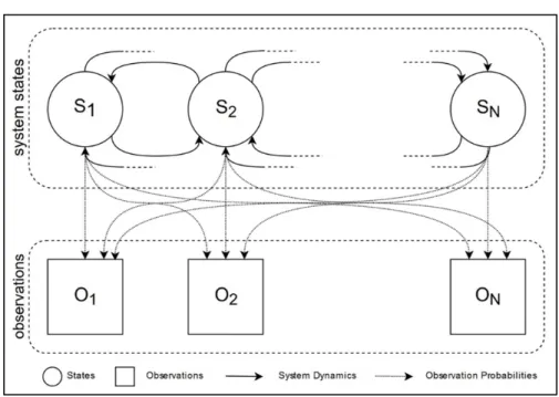
Figure 2.2: States space and observation space of a POMDP model
The state space and observation space of a POMDP model are depicted in Figure 2.2. In a POMDP, the states, actions, and observations can be discrete. We denote them at time by st, at, and ot respectively. Transition probabilities are action and state-dependent function: P(st+1, st, at) = pr{st+1| st, at}. The observation probabilities are a function of state, action, and observation: O(at, st+1, ot) = pr{ot|at, st+1}. Since the states are not directly observable, the decision maker’s belief about the current state of the system is represented by a belief stateπtwhich is a probability distribution over all possible states. The belief state is updated using Bayes’ rule every time an action is taken and an observation is observed: πt+1(st+1)∝ O(at, st+1, ot)
P
P(st+1, st, at)πt. The importance of the observations and their relations with the actual states is given in the belief state update formula based on Bayes’ rule where the function O is used. The more accurate this function is in terms of providing information about the actual state of the system, the better is the solution of the POMDP.
At each time step or decision epoch, the decision maker makes a decision and takes an action available from the action set. The decision maker takes this action based on the observation. The system then evolves into a new state, new observations are made, and the decision maker needs to take an action again. Each time an action is taken a certain amount of reward is given to the decision maker based on the given reward function R(st, at) which is action and state-dependent.
In POMDPs we are trying to find a set of actions (a policy) that maximizes (minimizes) the expected total discounted rewards (costs) over an infinite horizon. Such a policy is called the optimal policy. The optimal policy ℘∗ is obtained by solving the Bellman Optimality Equation V∗(π) = maxa∈A R(π, a) + λP o∈ΩO(a, π, o)V ∗(π0) .
The optimal value can be computed by applying dynamic programming to iteratively improve the value of the function.
Since the belief space is uncountable, the above dynamic programming recursion does not translate into practical solution methodologies. Even with the finite dimensional characterization of a POMDP (finite state space, finite action space and finite observation space), determining the piecewise linear segments of the value function at each epoch is computationally expensive due to the fact that the number of piecewise linear segments can increase exponentially with the action space dimension, state space dimension and observation space dimension. Therefore, exact computation of the optimal policy is only computationally tractable for small state dimension, small action space dimension and small observation space dimension. It is shown in Papadimitriou (1987) that solving a POMDP is a PSPACE-complete1 problem. Littman (2009) gives examples of POMDPs that exhibit this worst case behavior. It is inferred that simplifying a POMDP model in any way such
1Decision problem A is PSPACE-complete if both of the following are true (Sipser (1997)):
1. A∈PSPACE (PSPACE: Decision problems solvable in polynomial space) 2. For everyX ∈PSPACE,X ≤P A.
as reducing the dimension of any of the spaces including the observation space can save significant amount of computational expenses. In the next section, we will see how this problem of interest has been studied in the literature.
2.3. Literature related to Partially Observable Markov Decision Processes
Controlling a Markov process with incomplete state information (including a partially observable state space) was first studied in Dynkin (1965). The first POMDP model was developed in Drake (1962). Other researchers at the same time developed finite horizon POMDPs in the context of stochastic control problems (Aoki (1965); Astrom (1965)). During the past years many other generalizations and versions of POMDPs have been investigated and developed by researchers including POMDPs with an uncountable action space (Sawaragi and Yoshikawa (1970)), POMDPs with Borel spaces (Rhenius (1974)), POMDPs with an arbitrary core process state space (Furukawa (1967)), non-stationary POMDPs (Hinderer (1970)), undiscounted infinite horizon POMDPs (Platzman (1980)), semi-Markov core process PODMPs (White (1975, 1976)), and so on.
There also exists a large number of papers investigating Bayesian control of the sequential decision process including Furukawa (1967); Rieder (1975); Satia and Lave (1973); Wessels (1968).
In terms of dealing with observations and the observation space, not much research has been reported. Most of the studies that utilize POMDPs to solve their problems including Ayer et al. (2012a); Cassandra (1997); Grosfeld-Nir (1996); Hauskrecht (2000); Littman (2009); Monahan (1982); Sandikci et al. (2013) simply and naively assume that a single-signal is apriori known, not considering the fact that real-world systems produce a large number of signals and that the observation space plays a significant role in POMDPs where the current state has to be inferred through observations. There exist only a few studies that deal with how to select multiple observations from a multidimensional observation space. In Hoey and Poupart (2005) authors speak of multidimensional observation spaces, how to sample from them, and how to aggregate observations in order to reduce the dimensionality of the
observation space. Observations can be aggregated in some cases if the policies associated with them are the same (policy-directed observation aggregation). Observations can also be aggregated in one-dimensional continuous observation spaces by discretizing the continuum into segments whose observations yield the same optimal policy (Hoey and Poupart (2005)). For multidimensional observation spaces, authors in Hoey and Poupart (2005) examine two approaches. The first approach is for observation spaces where observations are composed of conditionally independent variables. For this case, they reduce the observation space to one dimension by sequentially processing the observation variables in isolation. The second approach which is used for arbitrary multi-dimensional observations is sampling and it is proved to be an effective approximation technique for computing aggregate probabilities. The authors in Hoey and Poupart (2005) propose a dynamic partitioning technique which is integrated with point-based backups. There are several drawbacks associated with these types of methods. These methods do not work with some POMDP algorithms such as Incremental Pruning (Cassandra et al. (2013); Zhang and Liu (1996)), Witness algorithm (Kaelbling et al. (1998a)), and Bounded Policy Iteration (Poupart and Boutilier (2004)). Another drawback is that the proposed method in Hoey and Poupart (2005) deals only with POMDPs with continuous observations but discrete states. Although others have tried to reduce the dimensionality of the whole POMDP by reducing the observation space’s dimensionality, they have never looked at the problem from a different perspective. All the efforts that have been made are post-POMDP dimensionality reductions. Here we apply a pre-modeling technique for observation aggregation that not only produces more meaningful and accurate observations from the system, but it also shapes both the state space and observation space in full compliance with each other.
2.4. Predictive Modeling for Observation Aggregation
Observations and their relations to the actual states in POMDPs are extremely important. Systems may produce more than one signal and these signals can be used as observations in POMDPs. The question of how to choose the signals to use as observations in a POMDP
is still open in the literature. If all signals are used as observations, we will have a large observation space which makes POMDPs very difficult to solve. Even if there is no problem with the dimensionality, determining the relationship between these many signals and actual states of the model is not always possible. As mentioned before, reducing the dimensionality of the observation space by aggregating the observations into more accurate and informative ones can save significant amount of computational expenses.
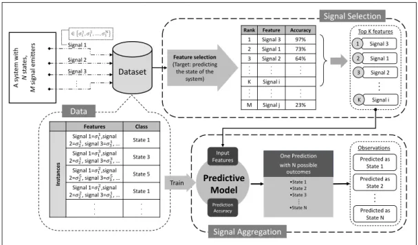
The fact that systems produce signals all the time (either continuously or discretely in time) reveals that the information from these signals gathered over time provides historical data for the system. If enough data is gathered from the sources of signals (enough signals recorded), the data can then be analyzed for further purposes using data-driven analytics techniques. One purpose is to select a subset of signals and aggregating them into a single more accurate and meaningful observation. This problem is broken down into two major steps in this research work. The first step is to select a proper subset of signals from the system (signal selection step). And the second step is to combine or aggregate the selected signals into a strong observation (signal aggregation step). These two steps are depicted in detail in Figure 2.3.
The first step is a feature selection problem. We try to select a subset of features (signals) that are later going to be used in a predictive model to produce more meaningful observations. From another perspective, using historical data recorded from the signals, in this step we identify which signals are giving more information about the actual states of the model. The outcome of this step would be a list of signals, sorted based on their strength in pointing to the right state of the system.
What needs to be taken into consideration in the signal selection step, is the problem of missing data. This matters because one type of signal may be accurate, but it might be harder to observe and thus not always available. We will later see in the signal aggregation step why this is important.
The signal aggregation step is implemented by a predictive model that uses the selected features from the previous step in order to provide outcomes that are more meaningful and
A s ys tem wi th N st at es, M signal em it ter s Dataset Features Class In st an ces Signal 1=𝜎11,signal 2=𝜎21, signal 3=𝜎31, … State 1 Signal 1=𝜎13,signal 2=𝜎21, signal 3=𝜎33, … State 3 Signal 1=𝜎12,signal 2=𝜎25, signal 3=𝜎35, … State 5 Signal 1=𝜎12,signal 2=𝜎22, signal 3=𝜎31, … State 1 . . . . . . Signal 1 Signal 2 .. .
Rank Feature Accuracy 1 Signal 3 97% 2 Signal 1 73% 3 Signal 2 64% . . . . . . . . . K Signal i . . . . . . . . . M Signal j 23% Signal 3 ∈ 𝜎11, 𝜎12, … , 𝜎1N Signal 3 1 Signal 1 2 Signal 2 3 Signal i K .. . Top K features Signal Selection Feature selection (Target: predicting
the state of the system)
Data
Predictive Model
Input
Features One Prediction with N possible outcomes •State 1 •State 2 •State 3 •State N .. . Predicted as State 1 .. . Observations Predicted as State 2 Predicted as State N Signal Aggregation Train Prediction Accuracy
Figure 2.3: Data-driven signal selection and aggregation framework
accurate. In this step, we develop a classification model where the input is the selected signals from the signal selection step and the classes are the actual states of the model. By training this classifier we will have a predictive model that takes all the signals as the input and then predicts the state of the system. These predictions are then used in the POMDP as observations to update the belief state.
Predictive models are rarely perfect. There are always misclassification errors associated with such models. These errors are taken into consideration and used as the relationship between the predictions (that are going to be used as the observations) and the actual states of the POMDP. In another word, the accuracy of the predictive model is implemented in the POMDP as the observation probability function.
Figure 2.3, shows an example system that has a total number of N states (i.e. card(S) = N) and the system produces M signal at each epoch. Each signal can take N distinct values (signal i ∈ σ1
i, σ2i, . . . , σNi ). This means that in a POMDP model that takes
card(Ω) = NM). Not all these N signal are perfect in pointing to the true underlying state of the system at each epoch. Some might work better than others. The strong signals are selected in the signal selection part of the framework. The predictive model then uses these signals to predict the state of the system. Although the prediction (the outcome of the predictive model) is in terms of the state of the system, it typically will not be completely accurate but can be used as an informative observation, increasing our understanding of what state the system most likely is in. Using the framework in Figure 2.3 we produce only one signal out of M signals, and this signal can take N distinct values (observations). Thus, the total number of observations will be N and therefore the size of the observation space is reduced significantly.
Chapter 3
Optimal Individualized Diabetes Screening (P1)
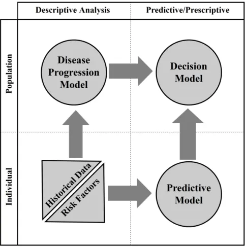
This chapter describes the application of the decision framework to the problem of diabetes screening. In this chapter, we provide details on the techniques used in the decision framework in Figure 3.1. We use POMDP to formulate the sequential screening decision-making problem. The model is informed by the population-specific disease progression learned from data using the HMM. The disease stages and the costs to the healthcare system and the patient are derived from the medical literature and clinical expertise. The screening decisions are highly personalized using a predictive model trained on a large set of electronic health record data. While any predictive model can be used, we apply here a logistic regression model with L1 regularization (LASSO). The solution of the POMDP given the assumptions is an optimal screening policy which can be used in clinical practice. We propose to supplement existing guidelines with an opportunistic screening strategy that (1) incorporates all clinical information available about each patient to identify individuals at higher risks of developing prediabetes or diabetes, and (2) identifies the optimal time to perform the screening to optimize expected health outcomes and healthcare cost. Figure 3.1 shows the high-level multi-method framework proposed in this paper. We use a POMDP model (upper right) to find an optimal policy for the main decision-making problems of whom to screen and when to screen/re-screen. The transition parameters of the POMDP model are estimated using a disease progression model (upper left), a Hidden Markov Model learned from historical patient data. The observations used by the POMDP model are created via a predictive model that incorporates patient-level risk factors (lower right).
Figure 3.1: Multi-method decision-making framework to combine progression modeling and predictive modeling with optimization
3.1. Background on Diabetes
Like many other chronic diseases, Type 2 diabetes has a prolonged asymptomatic period during which early detection is possible because diabetes onset occurs on average 9-12 years before clinical diagnosis Lu et al. (2010). Diabetes risk increases across a continuum with higher glucose levels corresponding to higher risk as the glucose level is an indicator of whether the patient has diabetes. For diagnostic and treatment purposes, two key stages are characterized – prediabetes and diabetes. In the prediabetes stage, patients are asymptomatic and blood glucose is higher than normal but not high enough to be classified as diabetes. Although progression to diabetes can be reversed by lifestyle modification and interventions like bariatric surgery, many patients with prediabetes go on to develop diabetes,
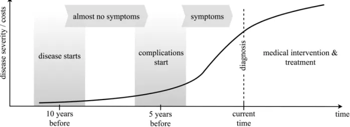
Figure 3.2: the costs associated with the disease increase very quickly as the severity of the disease increases
a chronic disease requiring medical treatment to control the disease and prevent/manage complications. Importantly, identification of patients during the prediabetes stage allows the delivery of evidence-based interventions to delay or prevent the development of diabetes prevention Program (2008); Group (2002). Thus, screening of individuals at risk for diabetes and timely surveillance of patients with prediabetes to detect the transition to diabetes is critical to improving health outcomes and reducing healthcare costs (see Figure 3.2).
Systematic diabetes screening and prevention programs can identify patients at risk for diabetes and target preventive interventions to delay or prevent the development of type 2 diabetes. The American Diabetes Association (ADA) and the US Preventative Services Task Force (USPSTF) provide physicians with guidelines for screening. These guidelines recommend screening about 70% of the population Calonge and Petitti (2008); Care (2013), which is a very expensive proposition and in many cases, operationally impractical Howard et al. (2010). The guidelines are based on only a as small number of predictors including age, body mass index, and a few risk factors. This results in a sensitivity as low as 65% for USPSTF and specificity as low as 23% and 67% for ADA and USPSTF respectively for identifying diabetes cases.
3.2. Related Literature
Figure 3.1 provides an overview of the methods used in this paper to address the problem of diabetes screening. Many of these methods have been employed independently to answer specific questions in the healthcare context but they have not been integrated to address such a decision-making problem. In the following, we review the literature related to these methods and techniques.
3.2.1. MDP for Medical Decision Making
Markov Decision Processes (MDPs) and Partially Observable MDPs (POMDPs) are methodological tool of choice to study medical decision making problems for chronic diseases such as Diabetes (Kuo et al. (1999); Santoso and Mareels (2001); Shih et al. (2007); Hoerger et al. (2004)), HIV/AIDS (Lee et al. (2014); Gafa et al. (2012); Shechter et al. (2008)), Cancers (Ayer et al. (2012b); Garc´ıa-Mora et al. (2010); Ahsen and Burnside (2018); Maillart et al. (2008); Chhatwal et al. (2010)) and their associated complications (Sandikci et al. (2008, 2013); Schaefer et al. (2004); Sukkar et al. (2012); Alagoz et al. (2010)). MDPs have also been used for hypertension treatment specifically for designing therapeutic regimens for patients with hypertension (Zargoush and Daskalopoulou (2018)). Also, MDPs have been used for a wide range of healthcare management problems such as dealing with emergency department congestion (Patrick (2011)). An attractive key feature of MDPs is that they can be used to deal with sequential decision-making problems in contexts with large levels of uncertainty (for example, in terms of how fast the disease progresses in a given patient population). In such settings, MDP’s can be used to determine the optimal time for screening and treatment initiation (Alagoz et al. (2010)). For example, MDPs have been used to answer questions such as: optimal time to initiate antiretroviral therapy in HIV patients (Shechter et al. (2008)), optimal time for breast cancer screening in women (Maillart et al. (2008); Chhatwal et al. (2010); Ayer et al. (2012b)), or optimal time for accepting a living-donor transplant in patients suffering from end-stage liver disease (Alagoz et al. (2004, 2005); Sandikci et al. (2013, 2008)). Readers are directed to (Alagoz et al. (2010); Monahan (2008); Cassandra
(1997); Schaefer et al. (2004)) for a review of literature describing uses of MDPs in medicine.
3.2.2. HMM to Model Disease Progression
Disease progression modeling is important for disease prognosis improvement, drug development, and clinical trial design. Difficulties with modeling disease progression include progression heterogeneity (patients have different progression trajectories due to many reasons), incomplete patient records (censoring and missing information), discrete observations (disease progression is a continuous process, but patients’ records of the progression are observed and recorded at discrete times with varied intervals), and irregularity of observations (due to irregular visits) (Wang et al. (2014)).
A large portion of the literature on disease progression modeling focuses on evidence-based modeling using machine learning and statistical techniques evidence-based on observational data. A popular model is the hidden Markov model, where disease progression is modeled as a progression through a set of unobservable discrete disease states governed by transition probabilities. For example, a general hidden Markov model to estimate transition rates between states as well as the probabilities of states of misclassification is presented in Jackson et al. (2003). Another study (Liu et al. (2015)) presents an effective learning method for continuous-time HMMs by dealing with the challenges of estimating the posterior state probabilities and the computation of end-state conditional statistics. In Sukkar et al. (2011) the authors develop a six-state HMM of Alzheimer’s disease which allows progression by one or two states or regression by one state using data from 595 subjects. They calculate the states transitions and conditional probabilities of being in each state using the developed model. The authors also propose an HMM for the Alzheimer’s progression in another study (Sukkar et al. (2012)) with the ability to identify more granular disease stages than the three currently accepted clinical stages for Alzheimer’s disease. Some studies use techniques other than HMMs to model the disease progression or obtain state transitions such as simulation (Lee et al. (2008)). Best practices on estimating the transition rates between states including techniques such as HMMs can be found in Denton (2018); Siebert et al. (2012).
3.2.3. Predictive Models in Healthcare
There is a growing number of studies using predictive models in healthcare decision making. These studies include the use of analytics in healthcare such as personalized diabetes management (Bertsimas et al. (2017)), chemotherapy regimens for cancer (Bertsimas et al. (2016)), hospital readmissions (Shams et al. (2015)), and healthcare screening decisions such as screening for Hepatocellular Carcinoma (Yuen and Lai (2003)), breast cancer screening (Maillart et al. (2008)), and HIV screening (Deo et al. (2015)). Studies on the use of predictive models for diabetes screening are reviewed in (Collins et al. (2011)) where the authors conduct a systematic review of the methodology of 39 studies and in (Jahani and Mahdavi (2016)) where the authors develop neural network models for diabetes prediction and compare with other models.
(Collins et al. (2011)) survey 39 studies with 43 risk prediction models that use 4 to 64 predictors including age, family history, body mass index (BMI), hypertension and fasting glucose. The most common modeling method among these studies is logistic regression. It is reported, that almost all reviewed studies remove incomplete cases or do not mention how missing data are treated. There are two types of predictive model in the literature, single-factor and multi-factor models. The single-factor models use common predictors such as age or BMI for which the availability in routine clinical settings is high. The drawback for single-factor predictive models is that no prediction can be made if the factor is not available for a patient. On the other side, for multi-factor models, can incorporate many factors, but since all these factors need to be available for the patient, for the sake of practicality a small number of predictors is typically preferred. Multi-factor models consider more information about the patient and therefore can provide better predictions compared to single-factor models.
The majority of the reviewed literature focuses on using a only single technique of the multi-method framework proposed in Figure 3.1. While these methods individually can be used to predict desease progression at the population level or what patients are more at risk of having undiagnosed diabetes, they only. . . The key contributions of this paper
is that we group all these methods and techniques together, using one to feed another, feeding all with real data to answer a question that has implications for clinical practice as well as contributions to a theoretical operations literature. Researchers have used the same techniques but independently, they have used MDPs or POMDPs to model decision making problems that concern healthcare but independent of what a specific hospital system would need or without using real data. They current state of the art is to simply assume some transition rates while we actually calculate using real data. They have used HMMs to estimate transition and progression rates for various disease but not in the context of a decision making problem. They have used data driven methods including predictive models to predict specific chronic diseases such as diabetes but never used it to feed MDPs as an individualized input for the decision making problem. . . . our approach is able to answer the questions of whom to screen, when to screen them and how often rescreening should take place in an integrated, analytics-driven decision framework that takes health outcomes, healthcare cost, cohort information, and available individual patient information into account.
3.3. The Partially Observable Markov Decision Process Formulation
Partially Observable Markov Decision Processes (POMDP) are an extension of Markov Decision Processes (MDP) to make optimal decisions when the current state of the system (in our case, the true health status of the patient) is not directly observable. The method uses a probabilistic belief distribution over the unobservable states of the system which is informed by observations. These Markov models assume that the process is Markovian, i.e., that future states only depend on the current state. While this is a very strong assumption, models based on the assumption are often very useful.
The set of states for the screening decision model are healthy, prediabetes, and diabetes. The decision is whether to screen the patient, henceforth referred to as “screening” decision. We assume the following: (a) the decision-maker is the clinician who acts on behalf of the patient and the health system, (b) the screening decision for a given patient is independent
of other patients, (c) screening decisions are made at discrete points in time when the patient and clinician meet, and (d) patients stay in each state for at least one decision epoch.
A discrete-time POMDP model is a 7-tuple (S, A, P,Ω, O, R, λ), where S is the set of states,A is the set of actions,P is the set of transition probabilities between the states, Ω is the set of all observations, O is the set of observation probabilities, R is the reward function of the model and λ is discount factor. Below are the detailed description of the essential components associated with the POMDP that need to be defined in advance to model the problem Cassandra et al. (1994); Kaelbling et al. (1998b); Puterman (2005):
3.3.1. Time Horizon and Decision Epochs
We use decision epochs of one year. Decisions are made at the beginning of each period starting from the first time the patient meets the clinician. We represent the epochs with t= 0, ..., T. The time horizon in our problem expands from the first time the patients meets the clinician until the patient dies or reaches the age of 79.
3.3.2. State Space
The state space in our model consists of a total of 7 distinct states S =
{H, P, D, SH, SP, SD,∆} and includes both observable and unobservable states. The 3
unobservable states are: Healthy (H), Prediabetes (P), Diabetes (D) which are the main underlying stages of diabetes. The 3 observable states are the screened representatives of the observable states: Screened Healthy (SH), Screened Prediabetes (SP), Screened Diabetes (SD). These states are completely observable, since they are the outcome of screening. The last state is Death (∆), which is the absorbing state.
3.3.3. Action Space
The action space, A ={S, N}, represents the decision to screen (S) or not to screen (N) a patient. We useat ∈Ato denote the action that is taken at time tat each decision epoch.
3.3.4. Transition Probabilities
These probabilities indicate the probability of a patient moving from the current state (st) to another state (st+1), given action at is taken. This probability is denoted by p{st+1 | st, at}. These transition probabilities are associated with the arcs on the Markov model underlying the POMDP (depicted in Figure 3.3). We use P to represent the set of all transition probabilities (typically one state-to-state transition matrix per action). Regression from diabetes to prediabetes or healthy states is very unlikely we therefore do not include an arc from state D to P or D to H, corresponding to a transition probability of zero.
For our model, we assume that the transition probabilities are stationary in the considered cohort. Thus, we drop the indextand use the notationp{s0 |s, a}to denote the “stationary” probability of transitioning to state s0 given the current state is s and action a is taken. A key characteristic of the transition probabilities is that the sum of the probabilities of transitioning from the current state to all other states including the current one should be equal to 1 for each single action; that is
X
s0∈S
p{s0 |s, a}= 1, for all s and a. (3.1)
We have the following:
p{H|H, N}= 1− X
s0∈S−{H}
p{s0 |H, N}= 1−p{P |H, N} −p{D|H, N} −p{∆|H, N},
(3.2) Similarly, for states P and D we have:
p{P |P, N}= 1− X
s0∈S−{P}
and
p{DH |D, N}= 1− X
s0∈S−{D}
p{s0 |D, N}= 1−p{H |D, N} −p{P |D, N} −p{∆|D, N}.
(3.4) We assume that a positive screening result (i.e., the patient is diagnosed with prediabetes or diabetes) influences the patient. The patient will receive medical treatment or may perform lifestyle changes (e.g., diet, exercising, weight loss). We capture these effects using the factors β, γ ∈(0,1) which are used to reduce the transition probabilities for the disease to progress from screened states (SP, SD) into more severe stages compared to patients in the same states but not screened.
3.3.5. Observations and Observation Probabilities
At each decision epoch, a signal/observation, o∈Ω, provides information about the true underlying (unobservable) state of the patient. Depending on the nature of the problem, observations can be obtained from various sources. We propose to create these observations using a predictive model (see Section 3.4) which classifies the patients into the groups of Predicted as Healthy (PH), Predicted as Prediabetic (PP) and Predicted as Diabetic (PD). Thus, the observation space is Ω = {P H, P P, P D}. Predictive models are usually not perfect and therefore the predictions used as observations are probabilistically connected to the unobservable states, i.e., the probability associated with predicting a specific observation o ∈ Ω, given that the true state of the patient is s is O(o | s) where O is the set of all observation probabilities.
3.3.6. Belief States
Π(S) is the probability simplex over the state space S, defined as Π(S) = {π ∈ R3 :
P3
i=1πi = 1, πi ≥0,∀i}, also called the belief space Sandikci et al. (2013); Brafman (1997); Sandikci et al. (2010). We useπtto denote the belief state at periodtwhich is the probability
distribution over the set of possible states, i.e., πt= (πt(H), πt(P), πt(D)).
3.3.7. Reward Functions
The POMDP maximizes expected rewards. Taking action a while being in state s will bring about an immediate reward denoted by the reward function r(s, a). We use as the values of the reward function estimates that combine the patient’s QALY (Quality Adjusted Life Year Neumann et al. (2014b) ), the costs of prediabetes, diabetes and screening tests all measured in US dollars. We formulate each state-and-action specific reward function from the societal perspective as follows:
r(s, a) = Q, s=H, a=N (1−αP)Q, s=P, a=N (1−αUD)Q, s=D, a=N Q, s=SH, a=N (1−αP)Q, s=SP, a=N (1−αDD)Q, s=SD, a=N (Q−CS)ur, s=H, a=S (1−αP)Q−CP −CS, s=P, a=S (1−αDD)Q−CD −CS, s=D, a=S (Q−CS)ur, s=SH, a=S (1−αP)Q−CP −CS, s=SP, a=S (1−αDD)Q−CD −CS, s=SD, a=S (3.5)
where the terms Cs, CD, CP, Q, le, ld, ur, Qand αi, i={P, U D, DD, D} are later described and estimated in Table 2 in section 4 alongside their values.
3.3.8. Bayesian Belief State Update and Optimality Equation
To implement learning from a new observationo, the belief stateπ= (π(H), π(P), π(D)) is updated to π0 using the Bayes’ rule. The updated component ofπ0 associated with state
s0 is given by π0(s0) = O(o 0 |s0)P s∈Sp{s 0 |s, a}π(s) P s0∈SO{o 0 |s0 }P s∈Sp{s 0 |s, a}π(s) (3.6)
Using belief states, the POMDP can be reformulated as a continuous state MDP and the optimal solution is the result of solving the Bellman optimality equations Puterman (2005):
ν(s, π) =maxa{r(s, a) +λ X j X s0 X o0 p{s0 |s, a}O{o0 |s0}ν(s0, π0)} (3.7)
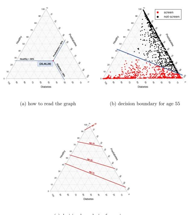
where λ ∈ [0,1) is the discount rate. The result will be the optimal screening program suggested by the model (see Section 5).
Figure 3.3: Underlying health states and observations of our POMDP model and the transitions among them. Only possible transitions are shown and those, which are not likely such as the transition from Diabetic to Healthy, are not depicted. Black arcs correspond to the natural progression of disease, green arcs correspond to the screening decisions, and red arcs correspond to reversion from screend states to uncontrolled ones.
3.4. Hidden Markov Models
A significant issue with using models that are based on transitions between unobservable states is how to estimate transition probabilities reliably from data. In our case, the states
H, P, D are not directly observable, but the POMDP models needs transition probabilities
between these states. The available data are provided by patient histories where at some point in time a diagnosis of prediabetes or diabetes is made, typically via a HbA1c screening lab test. We assume that up to the point in time when the diagnosis is made no significant medical intervention is performed and that the lab test reveals the true state (with some error). Transition probabilities between the unobservable states can be estimated from such data using a Hidden Markov Model (HMM), where the word hidden is used here for the fact that the true disease states are unobservable.
A HMM is a sequence of random variables Xt for time t = {1,2, ...} representing the hidden state with 3 possible values H, P, D and a sequence of associated random variables Yt whose realizations of the 3 possible values SH, SP, SD represent observations. There are two types of parameters associated with HMMs: the transition probabilities between two unobservable states given by the transition matrix
M ={mij}=P(Xt=j |Xt−1 =i), (3.8)
and the probabilities that indicate the likelihoods that a certain hidden state will lead to a specific observation in the form the emission probability matrix
N ={nj(yt)}=P(Yt=yt|Xt=j). (3.9)
The initial state distribution for t = 1 is defined as qi = P(X1 = i). The aim is to estimate the parameters of the hidden Markov chain,σ= (M, N, q) from observational data. The standard estimation procedure for HMMs is the Baum-Welch algorithm which utilizes the Expectation–Maximization iterative algorithm in order to find the maximum likelihood estimate of the parameters of the model given a set of historical observations Huang et al.
(2001). The transition matrixM provides a data-driven estimate for the transitions between the unobservable states in the POMDP specific to the cohort under consideration.
3.5. The Predictive Risk Model
Predictive risk models are powerful tools that can contribute to the decision-making process especially in the field of medical decision making. PRMs are usually multivariable, using several patient risk factors that are used to predict an outcome such as patient’s status. These models can be utilized in many different ways including identifying those who are at an increased risk of having an undiagnosed condition to target healthcare interventions or lifestyle changes to.
Instead of using different risk factors directly in the update of the belief state in the POMDP, we propose to use a predictive risk model (PRM) to generate personalized predictions (used as observations) for the POMDP. Using a PRM offers many attractive features including a wide selection of available classification methods, a simple and efficient learning process, the possibility of data-driven feature selection, and the availability of methods that deal with missing data. These are very important advantages for working with electronic health record data, where the amount of information available for each patient can vary substantially.
The PRM model is used to predict one of the K = 3 values for the response variable
G=H, P, D using a feature vectorx. Here we consider multinomial regression, an extension
of logistic regression for a response variable with multiple levels. The probability of value k is predicted by P(G=k|X =x) = e β0k+βkTx PK l=1e β0l+βlTx (3.10)
and the value with the highest probability is used as the prediction. The parameters are estimated from N observations yi using
minβ0,β 1 N N X i=1 l(yi, β0k+βkTxi) +λkβ k1, (3.11)
where the functionl calculates the negative log-likelihood contribution of observationi, and the last term is used for L1 regularization.
Predictive models make classification errors. For example, a healthy patient may be misclassified as having prediabetes. These errors can be assessed using standard cross-validation techniques and are typically summarized in a so-called confusion matrix. Since we use predictions as observationsoand the correct classification is given by the unobservable state s, the confusion matrix can be used as an estimate for the observation matrix O.
3.6. Parameter Estimation
In this section, we will first describe the data used in this research, and then we provide explanations on how we estimated each set of parameters using the techniques previously introduced and described in this chapter.
3.6.1. Data Description
The data used in this part of the research comes from the Electronic Health Record (EHR) of a large, integrated safety-net health system. Our cohort consists of patients from the Parkland Health & Hospital System, who are at risk for diabetes but have not been diagnosed with diabetes at the time of cohort entry. The cohort period is 2010 to 2014, during which individuals in the cohort may be diagnosed with diabetes. We retain patients, who have been diagnosed with diabetes, follow them over time, noting that additional information has been collected on them after their diabetes diagnosis. The cohort includes established primary care patients with an index visit occurring between January 1, 2012, and June 30, 2013, and 2 or more completed outpatient visits between the index visit and December 31, 2014. Patients are between 18 and 64 years of age at cohort entry. We exclude prevalent diabetes
Table 3.1: Key characteristics of the cohort studied
Entire Cohort (N=12071) Normal Glycemia (N=4883) Diabetes (N=1314)
Age, years (SD) 47.49 (10.5) 45.18 (11.1) 50.02 (8.9)
Female, % 69.9 69.8 68.2
Race/ethnicity Non-Hispanic White 13.3 15.2 10.2
Black 39.8 35.2 44.7
Hispanic 42 45 40.4
Other 4.9 4.7 4.7
Education, years, mean (SD) 8.73 (3.3) 9.06 (3.2) 8.15 (3.4) BMI, kg/m2, mean (SD) 31.37 (7.4) 29.74 (6.8) 35.2 (8.1)
Primary payer, % Charity 40 39 41.7
Private 13.2 13.1 11.8
Medicare/Medicaid 26.7 25 31.2
Self-pay 20 22.6 15.3
Lab values, mean (SD) Random Glucose 97.48 (17) 93.16 (12.9) 112.4 (27.3) HDL-C 51.74 (15.5) 53.65 (15.5) 47.57 (13.8) LDL-C 193.52 (38.6) 190.95 (38) 195.87 (39.4) Triglycerides 146.35 (99.4) 135.52 (86.6) 173.62 (136.3)
Systolic BP 129.11 (15.7) 126.01 (15.6) 135.44 (15.5) White Blood Count 7.39 (2.7) 7.34 (2.7) 7.71 (2.2)
Ferritin 140.06 (322.1) 140.26 (360.3) 150.95 (312.7)
Tobacco User, % Yes 12.2 12.8 12
Never 69.5 71.3 66.1 Passive 1.8 1.9 1.7 Quit 16.4 14 20.1 Alcohol User, % 10 9.9 10.2 Family history DM, % 71.1 74.8 62.1 Hypertension, % 46.9 38 62.6 CHF, % 2.3 1.7 3.8 Cardiovascular Disease, % 22.8 17.8 29.5
Medication use, % Steroids 18 18.6 17.6
Anti-hypertensives 45.5 37.4 61.5
and gestational diabetes. We excluded patients diagnosed with diabetes and prediabetes on or 18 months before the index visit using ICD-9-CM encounter codes, problem list diagnoses, and laboratory results (A1c, fasting glucose, oral glucose tolerance tests) meeting diagnostic criteria . Table 3.1 provides summary statistics.
We estimate various parameters of our model using the data described in Table 3.1. We reiterate that our goal is to provide an age-specific screening policy; some parameters such as mortality rates are estimated for various age ranges.
3.6.2. Estimating Transition Probabilities
We estimate the transition probabilities for the POMDP, using patients’ historical data (screening results from the EHR) as an input for the HMM. Screening results can be subject