Coordinated Control of VSC Based Multi-Terminal DC (VSC-MTDC) Power Grid

COORDINATED CONTROL OF VSC BASED

MULTI-TERMINAL DC (VSC-MTDC) POWER

GRID

by

Shimeng Huang

B.S. Tsinghua University, 2008

M.S. University of Pittsburgh, 2010

Submitted to the Graduate Faculty of

the Swanson School of Engineering in partial fulfillment

of the requirements for the degree of

Doctor of Philosophy

University of Pittsburgh

2015

UNIVERSITY OF PITTSBURGH SWANSON SCHOOL OF ENGINEERING

This dissertation was presented by

Shimeng Huang

It was defended on July 8, 2015 and approved by

Zhi-Hong Mao, Ph.D., Associate Professor Gregory Reed, Ph.D., Professor Ching-Chung Li, Ph.D., Professor

Thomas McDermott, Ph.D., Assistant Professor William Stanchina, Ph.D., Professor

Mingui Sun, Ph.D., Professor

Dissertation Advisors: Zhi-Hong Mao, Ph.D., Associate Professor, Gregory Reed, Ph.D., Professor

Copyright c by Shimeng Huang 2015

COORDINATED CONTROL OF VSC BASED MULTI-TERMINAL DC (VSC-MTDC) POWER GRID

Shimeng Huang, PhD University of Pittsburgh, 2015

Voltage source converter based multi-terminal DC (VSC-MTDC) system has raised great interest in academia and power industry. The maturing VSC technology has made such system possible for future medium and high voltage applications. Inspired by the success of DC based power distribution on electric ships, a number of VSC-MTDC systems have been proposed in literature for power grid innovation. However, there are still major technology obstacles to overcome before a VSC-MTDC grid come to utilization. Compared to the maturing technology on device level, research is still needed on the system and operation level. High dynamics and controllability of the VSC brings both opportunity and risks. Controllers must be carefully designed on grid level to fulfill multiple control objectives and coordinate local converter actions.

This work provides a comprehensive solution for MTDC system from modeling to control design. The procedure and tool sets are designed to be applied to various system setups and control schemes, so that it can be applied to multiple MTDC applications. First, thorough study on the VSC-MTDC system is conducted through analytical modeling and simulation. A systematic modeling method for general VSC-MTDC system is proposed. It contains a two-stage procedure that is generalizable to arbitrary system setup and configuration. A small signal state space representation which includes local and network dynamics can be obtained. A novel reconfigurable controller concept is then proposed to address multiple control strategies and communication constraints in system level. Design of such controller is formulated into a standard LMI optimization problem so it can be efficiently solved even

for large scale system. Using the proposed control design method, different control schemes can be easily explored through unified methodology and procedure. We demonstrated that existing control schemes for MTDC power balancing can be covered by this control structure. The proposed modeling and control design method is applied to four-terminal HVDC systems of multiple grid applications. Different control topologies and operation modes are evaluated and compared. Practical aspects such as LMI parameter tuning guideline and specifications for different applications are discussed.

TABLE OF CONTENTS

PREFACE . . . xii

1.0 INTRODUCTION . . . 1

1.1 BACKGROUND AND MOTIVATION . . . 1

1.2 RESEARCH OBJECTIVE . . . 3

1.3 CONTRIBUTIONS OF THE THESIS . . . 5

1.4 OUTLINE OF THE THESIS . . . 6

2.0 LITERATURE REVIEW. . . 8

2.1 CONTROL OF VSC-MTDC SYSTEM. . . 8

2.2 CONTROLLER STRUCTURE OF INTERCONNECTED SYSTEM . . . . 9

3.0 MODEL OF MTDC SYSTEM . . . 12

3.1 MODEL OF VSC SUBSYSTEM . . . 12

3.1.1 VSC connecting to AC power grid . . . 14

3.1.1.1 Current control inner-loop . . . 17

3.1.1.2 Real and reactive power control outer-loop . . . 20

3.1.1.3 AC voltage regulation . . . 23

3.1.1.4 DC voltage regulation . . . 28

3.2 MODEL OF DC CABLE NETWORK . . . 30

3.3 OPERATING POINT . . . 32

3.4 SUMMARY . . . 35

4.0 LMI-BASED CONTROL DESIGN . . . 36

4.1 RECONFIGURABLE STATE-FEEDBACK CONTROL FOR MTDC SYS-TEM . . . 36

4.2 LMI-BASED CONTROL DESIGN . . . 38

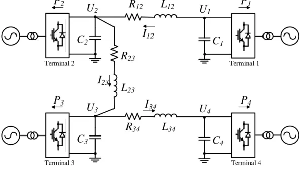
5.0 CASE STUDY OF A FOUR-TERMINAL SYSTEM INTERCONNECT-ING AC AREAS . . . 41

5.1 DISTRIBUTED VOLTAGE REGULATION . . . 43

5.2 PARTIALLY PARTICIPATING VOLTAGE REGULATION . . . 57

5.3 COORDINATED VOLTAGE REGULATION . . . 61

5.3.1 Voltage regulation by communicating local measurement. . . 61

5.3.2 Voltage regulation by full-state feedback . . . 68

5.4 SUMMARY . . . 70

6.0 CASE STUDY OF A FOUR-TERMINAL SYSTEM FOR OFFSHORE WIND INTEGRATION . . . 73

6.1 NATURAL DYNAMICS ANALYSIS . . . 74

6.2 POWER BALANCING CONTROL DESIGN . . . 76

6.2.1 Grid side voltage regulation. . . 76

6.2.2 Wind side voltage regulation . . . 80

6.2.3 Full participating voltage regulation . . . 82

6.3 SUMMARY . . . 85

7.0 CONCLUSIONS AND FUTURE WORK . . . 86

7.1 CONCLUSIONS . . . 86

7.2 FUTURE WORK . . . 88

LIST OF TABLES

1 Table of parameters . . . 42

2 Control effort and performance with different values of weight coefficient . . . 48

3 Control effort and performance with different H . . . 50

4 Norm of A’s row for state P1, U1, and DC currents . . . 53

5 Coordinated control effort and performance with different values ofa1 . . . . 63

6 Coordinated control effort and performance with different H . . . 66

LIST OF FIGURES

1 Abstract representation of research subject . . . 4

2 Abstract network representations of (a) a decentralized, non-cooperative con-trol architecture and (b) an entirely centralized concon-trol architecture. . . 10

3 Decompose the modeling of MTDC: (a) A MTDC system (b) A subsystem consists of a converter and its AC-side component . . . 13

4 Equivalent circuit of a VSC . . . 15

5 Control diagram of the inner-loop current controller . . . 17

6 Step response of an example VSC’s inner-loop control . . . 21

7 Control diagram of the outer-loop power controller . . . 22

8 Step response of an example VSC’s outer-loop control . . . 22

9 Equivalent circuit of a VSC connected to a weak AC system . . . 24

10 Diagram of AC voltage regulation compensator . . . 25

11 AC voltage regulation of example VSC connecting to a weak AC system. (a) Bode plot of the system with AC voltage compensator (b) Simulation result 26 12 Two control schemes of DC voltage regulation: (a) DC voltage PI control ind axis outer loop (b) DC voltage droop control . . . 29

13 UseK’s nonzero patterns to represent different controller structures . . . 37

14 Study case of a four-terminal system. . . 41

15 Eigenvalues of the open-loop system and their participating states . . . 44

16 Close-loop dynamics of the MTDC system withK in distributed form solved by LMI optimization: (a)Eigenvalues (b)Simulation. . . 45

18 Close-loop eigenvalue with different values of kKk listed in Table 2. . . 49

19 P2 response to -0.2 p.u. step change of P2∗ using different K . . . 49

20 Close-loop eigenvalue with different parameter matrixH and coefficient a1 . . 52

21 Close-loop system response to disturbance on different states at initial condi-tion: (a) 0.01 p.u. disturbance is added on U1 (b) 0.01 p.u. disturbance is

added on I12 . . . 54

22 Close-loop eigenvalue with different choices ofH . . . 56

23 Partially participating DC voltage regulation by Terminal 1 and 4. (a) Non-zero pattern of gain matrixK (b) Simulation result . . . 58

24 Corresponding eigenvalues for Figure 23(b) and their participating states. . . 59

25 Close-loop eigenvalue with different values of kKk, when Terminal 1 and 4 regulate DC voltage . . . 60

26 Coordinated DC voltage regulation: (a) Close-loop eigenvalue with different values of coefficient a1 (b) Simulation result when a1 = 0.4 . . . 62

27 Coordinated DC voltage regulation under different choices ofH: (a) Close-loop eigenvalue with different H(b) Simulation result when HU = 50 and HI = 2 65

28 Close-loop eigenvalues using full state feedback solved by LMI and LQR meth-ods . . . 69

29 Simulation result, Ksolved by (a)LMI method (b)LQR method . . . 71

30 Study case of a four-terminal system with wind generation. . . 73

31 Eigenvalues of the offshore wind integration system, and their participating states . . . 75

32 In operation mode 1, close-loop eigenvalues when weight coefficient a1

in-creases: (a) a1 from 0.001(blue) to 0.01(red) (b) a1 from 0.01(blue) to 0.1(red) 77

33 Simulation of operation mode 1: (a) a1 = 0.01 (b) a1 = 0.07 . . . 78

34 In operation mode 2, close-loop eigenvalues when weight coefficienta1 increases

from 0.001(blue) to 0.05(red). . . 80

35 Simulation of operation mode 2: (a) a1 = 0.001 (b) a1 = 0.05 . . . 81

36 In operation mode 3, close-loop eigenvalues when weight coefficient a1

37 Compare critical poles in operation mode 1(a) and 3(b), when weight coefficient a1 changes from 0.001(blue) to 0.01(red) . . . 84

PREFACE

I would like to express my most sincere and deepest gratitude to my advisor, Dr.Zhi-Hong Mao, for his support and guidance. He has been a great mentor in academia and a respectfully kind friend in life. I would also like to thank my co-advisor, Dr. Gregory Reed, for guiding me through amazing research projects and industrial collaboration, which have greatly inspired this dissertation.

I would like to further extend my thanks to my dissertation committee: Dr. Ching-Chung Li, Dr. Thomas McDermott, Dr. William Stanchina, and Dr. Mingui Sun. Their advise and support have motivated me to improve and complete this study.

In addition, I wish to thank my parents, Zhelin Huang and Weiping Ke, as well as my beloved family, for always being supportive to my choices and believing in me.

Finally, thanks to Junqing Wei, my soul mate and dear husband, for his love and respect, and for always inspiring me to become a better self. It has been a long and hard journey, but you make it filled with adventure and fun.

1.0 INTRODUCTION

1.1 BACKGROUND AND MOTIVATION

The past two decades witness the emerging of DC based power technology. With an ever increasing number of installation, systems like high-voltage DC (HVDC) and static compen-sator (STATCOM) have proved their merit in today’s power industry. Inspired by the fast development in power electronics and the worldwide growing demand on upgrading existing power systems, more innovative DC systems have been proposed. As a promising solution for renewable power integration, Multi-terminal DC(MTDC) system is one of the technology that is becoming a vibrate research area while also raise interests in power industry.

It is generally believed that the AC-DC voltage source converter (VSC) is to be used to construct a MTDC grid. This type of converter is a relatively new invention that utilize insulated gate bipolar transistor (IGBT) to have full control of gate switching. Compared to conventional current source converter (CSC), a.k.a line-commutated converter (LCC), VSC allows easier extension to MTDC and support various network topologies. Even in a back-to-back DC setup, VSC has the advantage of reducing requirement on AC stiffness and supporting change of power flow direction. In recent years, VSC has reached to maturity with increased power rating and efficiency, making VSC-MTDC possible for multiple high-voltage and medium-voltage applications.

The idea of medium-voltage MTDC power distribution was first proved on electric ship design, and is now taken to distribution grid by pioneering researchers [1]. The light-weight interface with AC and DC renewable source has made it an attractive alternative for micro-grid backbone. Quite a number of publications on VSC-MTDC are devoted to the application for off-shore wind power collection [2, 3, 4, 5, 6]. It becomes competitive choice against AC

grid due to the better property of underwater DC transmission cable. In the transmission area, some recent conceptual designs propose to use MTDC system for power sharing and frequency support among multiple AC areas [7, 8, 9]. A meshed MTDC supergrid is also believed to be the most possible backbone of a pan-European interconnected system that allows the massive integration of renewable energy sources in the system [10, 11].

Despite its great potential in the future power grid, VSC-MTDC still need to overcome major obstacles before coming to reality [10, 7]. Besides fundamental technical barrier like DC circuit protection, there are still many unknowns from the control and operation per-spective:

• Compared to existing power system structures, MTDC’s are mostly in conceptual and planning stage, we are in general lack of data, models and simulation tools to understand the system dynamics. There is also little knowledge on system’s transient and steady-state response to disturbance and faults.

• There is no determined control and communication architecture. It is a large design space to explore for engineering the system to desired function within realistic constraints.

• There is no standard for DC grid. Control and operation objectives are not as well defined as in AC grid.

• We are still lack of knowledge on the interaction between a MTDC and existing AC grid, and how it will impact the grid stability.

Generally speaking, high dynamics and controllability on the VSC terminals brings both op-portunity to improve dynamics of existing grid as well as risk of introducing undesired control conflicts, which may end up disturbing the overall system stability. Therefore, systematic procedure need to be developed to determine and weigh control objectives and design control and communication accordingly. Stability need to be considered carefully on the grid level. And control and communication structure must be able to coordinate the control action of all converters.

1.2 RESEARCH OBJECTIVE

The objective of this study is to modeling and study interactions among converters in a DC grid, develop a control design method that can coordinate local controllers to stabilize the grid and achieve optimal operation in system level.

The subject under study is a VSC-MTDC network, which can be connected with varieties of AC components, including local wind generation, loads(constant power loads and motors), and AC transmission lines connecting with other AC areas. Such system (Figure1(a)) can be applied as backbone of a microgrid or a DC segmentation out of future transmission network. The basic structure of the research subject is a meshed DC network shown in Figure3(a). It has VSC’s on edge nodes, serving the connection between DC and AC systems. And within the DC system, connections without converter are possible. This structure cannot support arbitrary DC voltage level transforming. Therefore DC-DC converters will be required when transmission is merging to distribution, or when the system contains DC storage or DC renewable sources (e.g. solar power). This leads to a more complex network with a hybrid of DC-DC and DC-AC converters (Figure 1(c)). Due to the lack of mature design of grid level DC-DC converter, existing research on multi-terminal DC system mainly focused on the basic DC network in Figure 3(a).

The essence of the problem is that there are multiple interconnected but physically distributed devices with fast dynamics and high controllability, each serves its own local performance objectives. Control must be designed in a way to coordinate their actions, so the local objectives can be achieved without threatening stability of the networked system. The feature of this work is that we consider the physically interconnected system as a whole instead of decomposing it into local subsystems. Stability issues imposed by interconnections will be studied. We then design a hierarchical control structure to both fit the distributed nature of the MTDC grid and coordinate the subsystems to stabilize the overall networked system. The main goal of this thesis is to:

First Establish analytical model for the full VSC-MTDC system. Then conduct thorough study on its dynamics.

Weak AC

grid

AC grid

grid

AC grid

VSC-MVDC

network

Motor

load/CPL

Renewable

generation

network

Other AC

component

VSC

AC

component

VSC

AC

t

DC source

component

DC source

or storage

Second Design a reconfigurable control architecture with corresponding optimization al-gorithm. So we can explore different control schemes through a unified methodology, and find the proper controller for the VSC-MTDC system to coordinate the converters’ action.

1.3 CONTRIBUTIONS OF THE THESIS

This study proposes a systematic and innovative procedure to model VSC-MTDC system and formulating control problems. The principles, procedure and controller structure developed from this study can be generalized to multiple MTDC applications. The main contributions of the thesis are:

• A systematic modeling method for general VSC-MTDC system. The procedure contains two stages that decouples modeling on local and network level. Moreover, all directional quantities are defined without loss of generality. So it can be applied to arbitrary system configurations with different network topology and various AC-side components. Addi-tional routines such as model assembling, adjustment and operating point solution are proposed to deal with various practical modeling issues.

• Identify local and global control objectives of MTDC systems, understand their couplings from a thorough study of existing local controls and applications of VSC.

• A novel reconfigurable controller concept based on state feedback control. It addresses multiple control topologies and communication constraints by setting feedback gain ma-trix into a set of nonzero patterns. Several existing control schemes can be covered under this unified formulation.

• Formulating the control problem into a standard LMI optimization so it can be efficiently solved efficiently by several third party tools. Practical aspects such as specification for different MTDC applications and convergence improvement are discussed.

• A detailed guideline of LMI parameters tuning for MTDC system control design. By tracking the movement of eigenvalues, different sets of parameters are identified to address

two main pair of trade-off: trade-off between control performance and cost; and trade-off between local and global control objectives.

In summary, this thesis provides a comprehensive solution for MTDC system from mod-eling to control design. The whole procedure and tool sets are designed to be applied to various system setups and control schemes, so that it can be applied to general MTDC studies.

1.4 OUTLINE OF THE THESIS

The study is conducted by analytical modeling, theoretical analysis and time domain simu-lations. The outline of the thesis is:

Chapter 2 A short literature review on converter technologies, VSC-MTDC control meth-ods and general control theories on interconnected systems.

Chapter 3 Propose a systematic and unified modeling method for general VSC-MTDC systems. It is a two-stage procedure that provides proper isolation between modeling at subsystem level and network level, so that it can be applied to arbitrary system configu-ration with different network topologies and various AC-side components. At subsystem level, existing VSC control schemes and applications are thoroughly reviewed, modeled and simulated. At system level, small signal state-space representation is derived.

Chapter 4 Several state space tools are introduced for MTDC analysis and control design. A reconfigurable state-feedback controller for MTDC system is proposed to address differ-ent control topologies and communication constraints. And a LMI optimization problem is formulated to solve the controller.

Chapter 5 The proposed modeling and control design method is applied on a four-terminal HVDC system. Four different control topologies is tested by configuring the gain matrix

K into different nonzero patterns in LMI algorithm. Under each control schemes, we demonstrate the tuning of LMI coefficients and study the resulting close-loop eigenval-ues and time domain performance.

Chapter 6 Another test case of off-shore wind integration is studied. The slow local dy-namics of wind farm connected VSC is modeled using our two-stage modeling procedure. The proposed control design method is then applied to address 3 possible operation modes of wind integration system.

2.0 LITERATURE REVIEW

2.1 CONTROL OF VSC-MTDC SYSTEM

Modeling and control of a single VSC has been extensively studied in the past two decades [12,

13, 14]. The most outstanding achievement is enabling the independent control of real and reactive power exchange, which has become the key feature of the converter. VSC-based technology on STATCOM and back-to-back power transmission has been proven to be of great merit. It is generally believed that DC technology can help improve the controllability of the power system. For instance, Clark et al. [15] propose to segment large AC grid with back-to-back HVDC interconnection, and use its controllability on power flows to prevent propagation of disturbance. However, when extended to multi-terminal system, the network topology somewhat downgrade the controllability on power flow. Van Hertem et al. [10] pointed out that though each terminal can independently control the power exchange between its AC and DC sides, flow congestion and DC voltage instability are still possible to occur. In fact, accurate power flow control is considered a major challenge of some MTDC system. In a DC power network, change of voltage is in fact capacity charging and discharging due to the change of power flow. In a back-to-back HVDC system, balancing of input and output power is done by setting one converter to DC voltage control mode [14]. It has long been suggested to extend this strategy to MTDC system by having one slack converter in DC voltage control mode so that the others can freely decide its power injection [6, 16,

8]. However, this design requires the slack converter to swallow all input/output power difference. Besides, there is no guarantee that the DC voltage on the rest converters would stay within a proper range for the VSC to operate [14].

Some other works [17,18] propose a distributed control scheme for the DC voltage, which let all converters share the task of power balancing. These works point out the similarity between AC frequency control and DC voltage control, and propose a simple droop control to achieve global power balancing by local observation and control. The benefit of droop control is to avoid conflicts between set values on distributed converters. However, unlike AC system, there does not exist a nominal voltage in a DC system. Chaudhuri et al. [19] have shown that local droop control may perform poorly because of this reason. To tackle this problem, Berggren et al. and Chaudhuri et al. [20, 19] propose to use global observation, which requires communication between converters.

Despite these efforts to improve droop control performance, it is after all a P controller. In AC system, secondary control (i.e. automatic generation control (AGC)) is required to complement its static error. The same control scheme is briefly suggested for DC system in [10]. However, the essential assumption of AGC is that the nominal frequency is the same in the entire interconnected system [21]. It can be implied that it is unlikely to directly transfer the primary and secondary control scheme onto DC system, especially for large scale DC grid. In a word, we believe there are great opportunities to explore innovative control design for the future MTDC grid. And it must be carefully designed to coordinate the control actions on all converters.

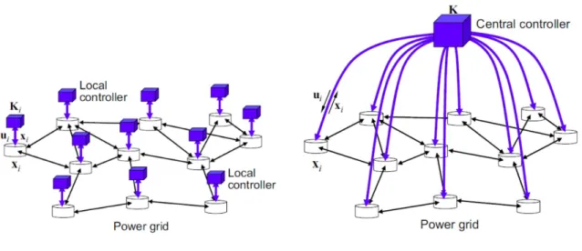
2.2 CONTROLLER STRUCTURE OF INTERCONNECTED SYSTEM

An MVDC system generally is a large, interconnected network. Mathematical description of this network involves differential and algebraic equations with a high-dimensional variable space. The network also requires the coordination of a large number of local actions. Either an entirely decentralized or centralized control structure cannot handle the high dimension-ality in MVDC control satisfactorily. Existing methods for on-line control are focused at the local level and are mostly decentralized, non-cooperative designs (Figure 2(a)). These de-signs can reduce dimensionality in control, but local controllers lack global observation of the subsystems in the MVDC grid and thus cannot achieve high performance network-wide [22].

(a) (b)

Figure 2: Abstract network representations of (a) a decentralized, non-cooperative control architecture and (b) an entirely centralized control architecture

In contrast, centralized control (Figure 2(b)) can achieve globally optimal performance, as-suming that the central controller has sufficient power of computation and there are no delays or losses of data during communication. However, the reality is that the control system must face both computational and communicational constraints. In particular, when communi-cation constraints such as time delays are present, a centralized architecture of control is potentially inferior to a tmore decentralized one [23].

Compared with entirely decentralized or centralized control, hierarchical control with cooperative components has been a more popular choice of control architecture [24]. A large body of existing literature has been contributed to the decentralized, cooperative control for large-scale systems (e.g., see survey papers and books [25, 26, 27, 28]). The optimal design of decentralized and cooperative control has been widely studied since at least the 1970s (e.g. [29,30,31]). In recent years, a trend has been to converge control, communication, and computation in the design of decentralized structure for networked control systems [32, 33]. In most of the existing research works, the topology of the control and communication

structure is known prior to synthesis, and optimal design for decentralized or distributed control is performed subject to this particular structure.

3.0 MODEL OF MTDC SYSTEM

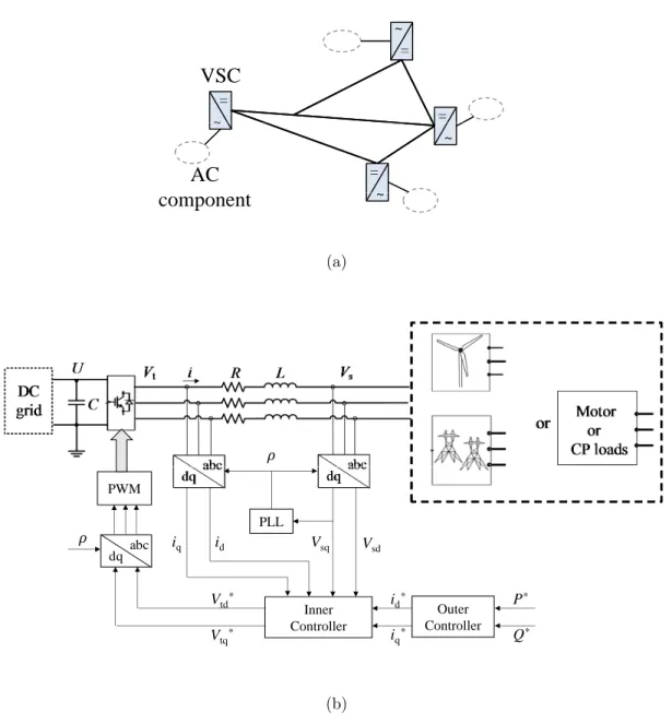
In this chapter, we introduce a systematic procedure to obtain small signal representation of MTDC systems. Figure 3(a) illustrates a typical MTDC system, which consists of multiple converters interconnected through DC cables. We assumed that all converters are VSC’s, and they each could connect to a different type of AC system, such as AC power grid, wind farm, and load, etc. The entire MTDC network can be divided into subsystems that are coupled through DC grid. A subsystem, as shown in Figure 3(b), is defined to represents the local dynamic of a converter together with its AC-side component. To obtain analytical model of the MTDC network, we follow a two-stage procedure: converter modeling and DC grid modeling. It provides proper isolation between modeling at subsystem level and network level, so that the modeling method is generalizable to arbitrary system configuration, such as different network topologies and various AC-side components for individual converters. Besides, the resulting model can be easily reconfigured when the system is changed, making it convenient to explore different designs of a MTDC.

In Section3.1, state space models of various VSC subsystems is derived and simulated. In Section3.2, DC network model is introduced, and subsystem models are assembled together into the overall system model. Finally in Section 3.3, a numerical routine is presented to solve the operating point of the small signal model.

3.1 MODEL OF VSC SUBSYSTEM

In the first stage of our modeling procedure, state space representations of each subsystem are derived. Note that subsystem-level control is also modeled at this stage. The state space

= ~ =

VSC

AC

component

Figure 3: Decompose the modeling of MTDC: (a) A MTDC system (b) A subsystem consists of a converter and its AC-side component

model is a set of first-order differential equations describing the subsystem’s small signal dynamic behavior, which can be expressed in a matrix form of

˙

xk =Akkxk+Bkuk+Bckuck, (3.1)

wherek is the index of the kth terminal in MTDC. In (3.1),xkis local state variables of the

subsystem, which are obtained from both AC-side and DC-side equations of terminalk. The inputs are divided into two groups: uk represents local inputs that can be determined within

a subsystem;uck are inputs that are influenced by other terminals, such as DC current flows

into or out of a converter. Variables in uck are temporarily modeled as input at this stage,

their dynamic behavior will be studied in Section 3.2.

Mathematical modeling for VSC connecting to varieties of AC systems can be found in the literature. These include stiff or weak AC grid [34, 35, 16], wind generation [36], and constant power load [37]. Like these works, we use average model [38, 13] to represent the converters in this paper. Switching of power electronics inside VSC is not modeled, because it is much faster than AC or DC-side dynamics under study. Converter’s average model provides sufficient approximation for the purpose of system stability analysis and control design while greatly reduced model’s complexity. In this section, VSC subsystem models for several major converter applications is introduced.

3.1.1 VSC connecting to AC power grid

We follow a modeling procedure similar to [13] to obtain (3.1) for VSC connecting to AC power grid. Equivalent circuit of the subsystem is shown in Figure 4. On the AC-side, VSC is connected to the grid through a phase reactor and a transformer. Together they can be represented by a combined impedance Z = R+jωL. On its AC-side, VSC can be viewed as a three-phase AC voltage sourceVt. So the basic equation of this circuit is :

Vt−Vs =Ri+L di dt,

R

L

R

L

i

V

V

I

m

n

I

C

U

C

U

DC side

AC side

P

P

PCC

Figure 4: Equivalent circuit of a VSC

The equation is then transformed to a synchronized rotating dq reference frame:

did dt =− R Lid+ωiq+ 1 L(Vtd−Vsd) diq dt =−ωid− R Liq+ 1 L(Vtq−Vsq) (3.2)

Note that the dq transformation projects three-phase quantities onto two orthogonal axes

d and q, which are rotating synchronically with PCC voltage Vs. The synchronization is

implemented by a phase-lock loop(PLL) that alignVs with one of the axes. In this paper, it

is arbitrarily assumed to be the d axis. As long as PLL remains stable, equation:

Vsd=|Vs| and Vsq= 0 (3.3)

always hold. The purpose of dq transformation is to reduce control complexity: First, it brings the three-phase quantities down to two-dimensional, leading to simpler control struc-ture; Second, the rotating reference frame transform sinusoidal signals to DC like quantities, which greatly reduces the requirement on controller bandwidth. As a result, control on dq

Real and reactive power output to AC grid can be expressed in dq-frame quantities by the following derivation:

P +jQ=Vs·i∗ = (Vsd+jVsq)(id−jiq) = (Vsdid+Vsqiq) +j(Vsqid−Vsdiq) (3.4) Substitute (3.3), we got P =Vsdid Q=−Vsdiq (3.5)

AC and DC-side dynamics of VSC is related through the conservation of real power. As shown in Figure 4, when ignoring the loss on switching and phase reactor, real power entering the converter’s DC-side should equal to that being injected to AC grid, i.e.

Pdc=Pac =P.

While P is expressed in (3.5) on the AC-side, it should subject to the following relation on DC-side: real power taken from DC grid at terminal k is the sum of the power converted to AC and the instant charging on large capacitor Ck. This derives:

dUk dt =− 1 Ck P Uk + 1 Ck Ik.

The nonlinear DC-side equation can be linearized around operating point P0 and Uk0 as dUk dt =− 1 CkUk0 P + P0 CkU_k2₀ Uk+ 1 Ck Ik (3.6)

Combining (3.2),(3.5),and (3.6), we have the open-loop state space model of a converter connecting to a strong AC grid in form of (3.1):

      ˙ idk ˙ iqk ˙ Uk       =        −Rk Lk ωk 0 −ωk −R_Lk k 0 − Vsdk CkUk0 0 Pk0 CkUk20              idk iqk Uk       +       1 Lk 0 0 _L1 k 0 0         Vtdk−Vsdk Vtqk−Vsqk  +      0 0 1 Ck      Ik (3.7)

Since the object of this research is MTDC grid-level control, the converter-level controllers are considered as part of the modeling work. Instead of designing innovative control scheme

PI

PI

Figure 5: Control diagram of the inner-loop current controller

for converters, we just model the behavior of existing controllers that are commonly used in VSCs. A common control design for VSC contains two cascaded control loops: a current control inner-loop and an application-specific outer-loop. Feedforward decoupling technique and PI controller are used to achieve independent control of real and reactive power that is being exchanged with the AC grid. The controllers are introduced and close-loop model of the subsystem is derived in the following sections:

3.1.1.1 Current control inner-loop We first assume the AC system is stiff, so voltage

Vsd and Vsq remains constant. The current i that flow through phase reactor can then be

controlled through converter’s AC voltage Vtd and Vtq, which is the control input of VSC.

Figure 5 shows the block diagram of inner controller. It contains a cross feedforward compensate path to cancel out the coupling term between d axis and q axis in (3.7). The decoupled open-loop system has first order dynamics between i and Vt on both axes, each

can be controlled by a PI controller. Ondaxis, to haveid tracking a reference valuei∗d, inner

controller takes the control error and output a set valueV_td∗. The same structure is also used onq axis. The two control outputs can then be transformed back to a three-phase quantity. Note that the set value of Vt still need to be transformed into PWM signal and executed by

To model the close-loop system with inner PI controller in state space, augment the open-loop model (3.7) with stateszintroduced by the I controllers, i.e. the integrated errors ond and q branch:   ˙ x ˙ z  =   Ax+Bu y−r  =   A 0 C 0     x z  +   B 0 0 I     u r   (3.8) in which r= h i∗_d i∗_q i>

is the reference in Figure5 and

x= h id iq U i> , u= h Vtd Vtq i> A=        −Rk Lk 0 0 0 −Rk Lk 0 − Vsdk CkUk0 0 Pk0 CkU_k2₀        , B=       1 Lk 0 0 _L1 k 0 0       , C=hI 0 i

are from (3.7). Since inner-loop control is purely local, all terminal indexes are removed from states for simplification, and the coupling term with other terminals is also omitted. Moreover, compared to (3.7), termωk is canceled inAby the cross feedforward paths shown

in Figure 5, and AC system voltageVs is also cancelled in u.

Next introduce control parameters kP and kI, so that the PI controllers in Figure 5 are

written in form kP+ kI

s . In the close-loop system, we can then expressu in (3.8) as a linear

combination of states and references:

u=−   kP 0 0 0 kP 0  x−   kI 0 0 kI  z+   kP 0 0 kP  r =−hkPI 0 i x−kIIz+kPIr (3.9)

Substitute (3.9) into the augmented system (3.8), we can derive the state space expression of close-loop system ˙ xc =Acxc+Bcr, (3.10) in which xc = h x z i>

Ac=   A 0 C 0  −   B 0   h kPI 0 kII i , Bc =   kPB −I  

At this point, we get the model of VSC with inner-loop control. While other parameters are from system specification, control gains kP and kI need to be picked. And they can

be chosen following a well established method [13, 14]. It is introduced next as part of subsystem modeling. From (3.10), we can derive the close-loop transfer function betweenid

and iq and their references. Since close-loop dynamics on d and q axes are decoupled and

identical, we arbitrarily use id in the following derivation: Id(s)

I∗

d(s)

= G(s) 1 +G(s) in which the loop gain is

G(s) = (kp+ ki s) 1 Ls+R = ( kp Ls) s+ki/kp s+R/L.

Note in the denominator that the VSC has a pole determined by phase reactor parameters:

s=−R

L.

Common values of R and L make this pole very close to zero. So a compensator zero is usually used to cancel it out, and thus we have

ki kp

= R

L (3.11)

After the zero pole cancellation, the close-loop transfer function of id becomes Id(s)

I_d∗(s) =

1 (L/kp)s+ 1

,

a first order system with time constant

From (3.11) and (3.12), we can derive the rule by which proportional and integral gains of inner control can be calculated from phase reactor parameters and expected close-loop time constant: kP= L τi , kI= R τi . (3.13)

Time constant τi is usually selected very small for fast current tracking response. It

can be arbitrarily small with the only constraint that the current controller dynamics must be sufficiently slower than switching frequency of power electronics. It is suggested that bandwidth of the close-loop system is smaller than 1/10 of the VSC’s switching frequency in rad/s. Typically, τi ranges from 0.5ms to 5ms for a VSC [14].

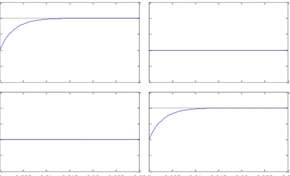
Figure6 shows the step response of an example VSC withR=0.0015p.u.,L=0.15p.u. at base value 100kV, 200MVA and 60Hz. A 5ms time constant is used for inner controller. It shows that, under inner-loop control, id and iq are fully decoupled, and each can track its

reference at expected speed.

Now we have fully derived the average model of VSC with inner-loop current control which can be used for subsystem simulation. However, it may not be controllable due to the zero pole cancellation in(3.11). To apply state space design methods to the system, an equivalent minimal realization is also derived to guarantee controllability and observability. Written in form of (3.1), we have:

      ˙ idk ˙ iqk ˙ Uk       =        − 1 τik 0 0 0 − 1 τik 0 − Vsdk CkUk0 0 Pk0 CkUk20              idk iqk Uk       +       1 τik 0 0 _τ1 ik 0 0          i∗_dk i∗_qk   +      0 0 1 Ck      Ik. (3.14)

3.1.1.2 Real and reactive power control outer-loop Reference value of the inner controllerid andiqis set by the outer controller. The purpose of this outer-loop is to control

real and reactive power P and Q being exchanged between VSC and its AC side. Based on (3.5), as long as Vsd is relatively well regulated, real power P is determined by id while

reactive power Qis determined byiq. As a result,P and Qcan be independently controlled

-1 -0.5 0 0.5 1 1.5 From: i_d* (pu) T o : i d ( p u ) 0 0.005 0.01 0.015 0.02 0.025 0.03 -1 -0.5 0 0.5 1 1.5 T o : i q ( p u ) From: i_q* (pu) 0 0.005 0.01 0.015 0.02 0.025 0.03 Step Response Time (seconds) A m p lit u d e

Figure 6: Step response of an example VSC’s inner-loop control

Figure 7 shows the diagram of VSC’s outer controller. Either real or reactive power control contains two parts: 1) a feedforward branch that directly calculates reference current using (3.5); 2)an optional feedback control loop that eliminates control error in case mea-surement of Vsd is not accurate. The two controllers work in parallel, or only the open-loop

control is used for simplicity. In general, dynamics of real and reactive power control is dominated by the faster feedforward control.

i∗_d = P ∗ Vsd + (kpp+ kii s )(P ∗ ₋ P) i∗_q=−Q ∗ Vsd −(kpp+ kii s )(Q ∗₋ Q) (3.15)

(3.15) is the mathematical description of Figure 7. Due to the immediate reaction of feedforward control, PI control parameters kpp and kii are usually picked small and can be

PI

PI

Figure 7: Control diagram of the outer-loop power controller

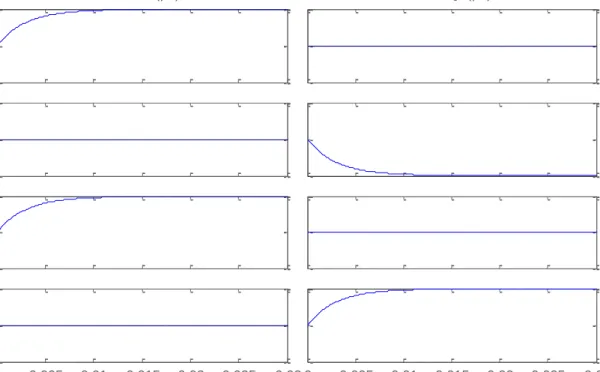
-1 0 1 From: P* (pu) T o : i d ( p u ) -1 0 1 T o : i q ( p u ) -1 0 1 T o : P ( p u ) 0 0.005 0.01 0.015 0.02 0.025 0.03 -1 0 1 T o : Q ( p u ) From: Q* (pu) 0 0.005 0.01 0.015 0.02 0.025 0.03 Step Response Time (seconds) A m p lit u d e

also introduce two extra states. The state space expression of the close-loop system can be obtained using the same augmented equation in (3.10). For outer control, plant matrices A

and B are that of the close-loop inner system, while

C=   Vsd Vsq 0 Vsq −Vsd 0  

is the observation matrix for real and reactive power. For close-loop system of outer control, the new input u =

h

P∗ Q∗ i>

is the power references. And the feedforward branches can be easily added to input coefficient matrix Bc of the close-loop model.

Figure8shows the outer-loop response to step change of real and reactive power reference. It is the same example VSC in section 3.1.1.1, with R=0.0015p.u., L=0.15p.u. And a 5ms time constant is selected for the inner controller. It shows that P and Q can be controlled independently by the outer controller. And they each track their references at the same speed of inner controller. This is because of the feedforward control can instantly calculate the input to inner controller.

It is noted that this fast open-loop effect cannot be represented by eigenvalues of close-loop system matrix. To capture this first order dynamics in further system analysis and control design, we also derive an equivalent minimal realization:

      ˙ Pk ˙ Qk ˙ Uk       =        − 1 τik 0 0 0 − 1 τik 0 − Vsdk CkUk0 0 Pk0 CkUk20              Pk Qk Uk       +       1 τik 0 0 _τ1 ik 0 0          P_k∗ Q∗_k   +      0 0 1 Ck      Ik. (3.16)

3.1.1.3 AC voltage regulation Reactive power tracking is usually not a direct control goal for a VSC subsystem. When connecting to stiff AC systems, reference Q∗ is usually constant zero. However, when it is connected to a weak AC network, of which the AC voltage level is not constant at PCC, the reactive power control on q axis can be used to regulate AC voltage Vs.

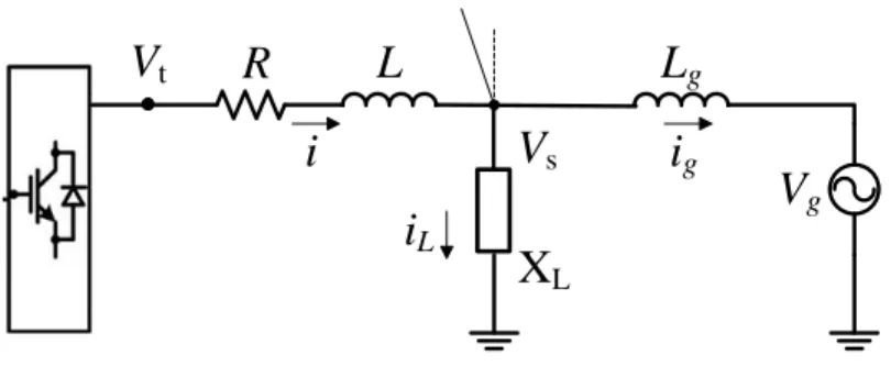
Figure 9 shows the circuit we use to simulate a weak AC connection. Inductor Lg is

added between PCC and the ideal voltage source so Vs at PCC becomes a variable. And a

R

L

i

V

V

I

m

n

I

U

Cj

U

L

C

V

i

C

R

L

i

V

V

L

V

i

i

X

R

L

PCC

PCC

Figure 9: Equivalent circuit of a VSC connected to a weak AC system

The strength, or weakness, of an AC system is measured by short circuit ratios(SCR). It is defined by SCR = S/Pd, in which S is PCC’s three phase short circuit level in MVA

at nominal AC system voltage Vs0, and Pd is the VSC’s rated DC power in MW. An AC

system is considered stiff when SCR > 3.0, weak when 2.0 < SCR < 3.0, and very weak when SCR<2.0. From its definition, we can derive that the test circuit’s SCR is determined by per unit value of Lg (base value Vs0,Pd and ω0, where ω0 is the nominal value of angular

velocity at PCC): SCR = V 2 s0 ω0Lg·Pd = 1 Lg(p.u.) .

For a weak AC connection, when the PLL remains stable, an extra I controller on the

q axis control branch(Figure10) can regulate AC voltage Vs [39, 14]. With the assumption

that PLL is stable, (3.3) is still valid. So Vs regulation is equivalent to Vsd regulation. The

compensator shown in Figure 10 is to be in cascade with the reactive power control outer loop. The output of the I controller sets the reference value Q∗ for the outer controller.

In this design, the outer and inner controller structure remains the same as for stiff AC system. Even though the inner loop control (Figure 5) treats ω and Vsd as constant for

decoupling an compensation, these two variables can also be measured in real-time for this purpose. It is also mentioned in [14] that nominal value ω0 can be used instead to still

get good decoupling result. However, this requires good regulation of Vs. The close-loop

I

∗

∗

Figure 10: Diagram of AC voltage regulation compensator

The AC voltage regulator in Figure 10is verified in our test circuit. The same example VSC is used, parameters: R=0.0015p.u.,L=0.15p.u. at base value 100kV, 200MVA and 60Hz. Real and reactive power controller is tuned to have 5ms time constant. For the weak AC circuit, set Lg=0.5p.u. so SCR is 2.0. And the integration gain for Vsd control is

tuned by Bode plot of the system, shown in Figure 11(a). Considering the characteristics of disturbance on load is often unknown in practice, large phase margin of about 90◦ is chosen for good robustness. Figure 11(b) plots the simulation result. A set of events is tested in this run:

• At 0.1s a 0.1p.u. step change is placed on V_sd∗ to show the step response of voltage regulation. It shows slower response than inner controller to reduce its influence on current control.

• At 0.7s a 0.1p.u. step change happens on P∗ to show that the real and reactive power control is still decoupled around the operating point.

• At 1s a gradual and then at 1.8s a step load current disturbance are introduced to show AC voltage can be regulated under small disturbance.

It is noted that there are limitations and conditions for this AC voltage control to work well. First it uses PLL, so dynamics ofVscannot exceed the bandwidth of PLL or it becomes

unstable. Second its stability is proved around an operating point of Vs and P. While Vs

is supposed to be regulated to a certain value, this condition limits the capability of real power tracking to relatively small bias from the real power operating point. Even though the real and reactive power control is still independent in the inner controller’s perspective, fast

−100 −80 −60 −40 −20 0 20 Magnitude (dB) 101 102 103 104 −180 −135 −90 Phase (deg) Bode Diagram Frequency (rad/s) (a) 0 0.5 1 1.5 2 1 1.05 1.1 1.15 V s d (pu) V_sd V_sd* 0 0.5 1 1.5 2 −1 −0.95 −0.9 P (pu) P P* 0 0.5 1 1.5 2 −0.1 −0.05 0 iLq (pu) (b)

Figure 11: AC voltage regulation of example VSC connecting to a weak AC system. (a) Bode plot of the system with AC voltage compensator (b) Simulation result

and large real power change at PCC imposes disturbance on Vs that can cause instability

on PLL. As a result, this voltage regulator is most commonly used on STATCOM, a VSC for the sole purpose of AC voltage regulation instead of real power exchange. Stand alone AC voltage regulation equipment like STATCOM is often added to a weak AC connection in addition to the converter to improve stiffness on the AC side. We find this AC voltage control through q axis works well in simulation with proper ramping or saturation of ∆P∗

for SCR >2.0. For very weak AC system, real power transmission level is further limited, VSC connecting to system with SRC = 1 can only transmit 0.4p.u. power using traditional controller [40].

When connecting to a very weak AC system whose SCR < 2.0, innovative control of VSC is still an active research topic. The main difficulty is to understand and control PLL’s transient under large disturbance of Vs. Durrant et al. [41] derived an average VSC model

which includes linearized PLL dynamics. However, due to the high order and nonlinear nature of PLL, such model stands only within very tight operating boundary. In our simu-lation, we also find it very hard to get good approximation of very weak AC system using just one linear model. Farag et al. [42] uses a similar linearization method but obtained multiple linear models around 52 operating points. An LMI method is then used to design a robust controller for these operating points. Such method requires intensive modeling effort on a single subsystem, thus can be very challenging to generalize for multi-terminal system. Besides the effort on detailed PLL modeling and control, another recent trend is to find alternatives to PLL [35, 43, 40, 44]. In [40] a model predictive control approach is intro-duced by Beccuti et al. to achieve real power control, AC voltage regulation and dq frame synchronization through one MIMO controller. While in [35, 43], Zhang et al. proposed to directly control the phase and magnitude of Vs so that dq frame alignment is not needed.

Under this control, the VSC shows similar dynamics as a synchronous machine and enables 0.86p.u. power transmission from a system with SCR = 1.2 in simulation. This controller is verified in [44] through simulation to integrate offshore wind generation by a VSC-HVDC link to a weak AC.

Since these new control concepts are still evolving and to be verified in industrial im-plementation. Only the traditional control method in Figure 10 is modeled in this work.

AC voltage regulation is considered a local control goal and is not coupled to real power control because detailed transient of PLL is not modeled. Instead, limitation on real power operating point and magnitude of ∆P∗ is considered as extra control requirements on the subsystem containing a weak AC. Moreover, ramping of P∗, if wanted, can be equivalently modeled by a larger time constant on the real power control.

3.1.1.4 DC voltage regulation Voltage regulation on DC side plays an important role in a VSC based DC system. One can see on the DC side of Figure4that voltageUk indicates

the charging of large capacitor Ck. When Uk increase, Ck is charging, implying that the

DC grid is accumulating power. On the other hand, when Uk decrease, Ck is discharging,

implying that the DC grid is loosing power. In other word, DC voltage is the indicator of power balance in a DC network, comparable to frequency in an AC grid. And thus the DC voltage regulation is thus as critical as primary control in AC system.

Since only real power is exchanged between AC and DC side of a VSC, DC voltage can be controlled through P control branch on d axis. This means that the two important control goals: real power tracking and DC voltage regulation, are controlled through the same input

V_td∗ of VSC. So some mechanism is needed to select or weigh between the two.

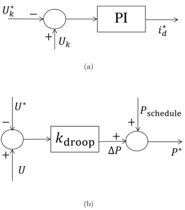
In a two terminal DC system, such as traditional HVDC or MVDC connection, power control and voltage regulation can be simply divided onto rectifier and inverter. Since the system is to transmit desired amount of power stably through a single DC link, it is common to have one terminal working in power tracking mode and the other in DC voltage regulation mode. In DC voltage regulation mode, outer controller ondaxis is replaced by a PI feedback control ofUk, which is shown in Figure12(a). This controller directly set reference for inner id controller. And a negative sign is added to control error because our defined positive

direction of id and P is discharging the DC side.

In an MTDC system, control strategies for power balancing is still an active research topic:

• One earlier control scheme is the slack converter method, which is directly generalized from two terminal technology. Using this method, we have N −1 converters out of a

PI

Δ

Figure 12: Two control schemes of DC voltage regulation: (a) DC voltage PI control in d

axis outer loop (b) DC voltage droop control

to be the “slack” that works solely on DC voltage regulation. The control of the slack converter is the same as that in traditional HVDC system (Figure 12(a)). This is the basic power balancing scheme commonly adopted in MTDC researches [6,45,16,46]. It is very simple but with obvious disadvantages. First the voltage regulation VSC takes all power disturbance in the system, which can impose great stress to its AC side frequency and voltage stability. Second, no power transmission can be scheduled for this voltage regulation VSC. Last but not least, there is no redundancy for DC voltage regulation in the system in case of fault or failure on the slack converter.

• To share the task of power balancing among multiple terminals, a voltage droop control method has been proposed in several papers[18, 17]. This control structure is adopted from primary control of AC frequency regulation. Figure12(b)shows one implementation of such droop controller. The droop gain kdroop is basically a P controller which take

the DC voltage error and generate a small adjustment ∆P on scheduled power reference

Pschedule. The two are combined as real power reference P∗ for the outer controller. The

reason for using only a P controller is to allow some control error. Due to their tightly coupled DC sides, such control error can avoid conflict among terminals. This allows the controller in Figure 12(b) to be deployed on multiple VSCs in an MTDC system. DC side dynamics is determined by the overall MTDC system, so we consider DC voltage regulation as a global control goal. The control design and performance will be studied after deriving the full model of MTDC.

3.2 MODEL OF DC CABLE NETWORK

In the second stage, models of subsystems are assembled into one system level model. At this stage, we first use circuits laws to derive state space model of the DC cable network. This introduces a new set of state variablesxc, which represents the couplings among subsystems.

An example of this type of state variables is the current on DC cables. Based on the coupling model, uck from stage one can now be expressed as a set of functions of xc:

uck =F(xc).

Then we can connect the subsystems by substituting these equations to (3.1).

In this paper,π-circuit is used to model DC connection between two nodes in the network. The capacitors in theπ-circuits combines both cable capacitor and VSC’s DC side capacitor, while value of the later is dominant. Equivalent circuit of the DC cable network is shown on the DC side of Figure 4. without loss of generality, we define all current flows from nodes with lower index to nodes with higher index. If the actual current is in the opposite direction, its value will be negative in our model. For the DC circuit network, current through inductor and voltage across capacitor are the natural choice of state variables. As dynamics of Uk is

already modeled in subsystem level, we only introduce new states:

xc=

h

· · · ijk · · · i>

Each DC connection will introduce one state variable. So the length of vector xc equals to

the total number of DC branches, nbranch, in the network. We then derive the dynamics of

allIjk, and use them to re-express the coupling inputIk in the subsystem model: dIjk dt =− Rjk Ljk Ijk + 1 Ljk (Uj −Uk) Ik = k−1 X j=1 Ijk− nbranch X j=k+1 Ikj (3.17)

For a general network topology, it is possible to have intermediate nodes that are in the joint of multiple DC cables but not in connect to a VSC. However such topology is rarely used in existing MTDC design and studies. So such intermediate nodes are not considered in our model for simplification of expression.

State space representation of a N-terminal DC system can be assembled by stacking up local statesxk from index 1 to N, then arranging coupling states xc at the end of the state

vector. The resulting linear model would take the form:

           ˙ x1 ˙ x2 .. . ˙ xN ˙ xc            =            A11 0 · · · 0 A1c 0 A22 · · · 0 A2c .. . ... . .. ... ... 0 0 · · · AN N ANc Ac1 Ac2 · · · AcN Acc                       x1 x2 .. . xN xc            +            B1 0 · · · 0 0 B2 · · · 0 .. . ... . .. ... 0 0 · · · BN 0 0 · · · 0                    u1 u2 .. . uN         . (3.18)

In (3.18), system matrix is mostly block diagonal with sparse coupling elements on the side. Subsystem matrix Aii can be of different dimension depending on type of AC system and

level of modeling detail of terminal i. Input matrix is also a block matrix because all control inputs are local and cannot directly effect states of other terminals. The all zero rows at the

bottom have the same number of rows as xc’s dimension. This indicates that no input can

directly affect coupling states in DC network.

The two-stage model generation method is implemented in a MATLAB script and can be applied to arbitrary MTDC setup. Moreover, the resulting state space model can be easily adjusted or reconfigured. When there is a change in subsystem i, we can simply changeAii

and Bi. Even dimension change in Aii can be easily handled with adding or removing all

zero rows inAicand columns inAci. Similarly when change is wanted on DC network, either

parameter or topology, it can be implemented by adjusting a few coupling elements on the side of system matrix without disturbing the subsystem models. This enables researchers to conveniently explorer different system setups and make adjustment on their MTDC design.

3.3 OPERATING POINT

For an N-terminal MTDC system, (3.18) is a linear small signal model around operating point

h

P10 · · · PN0 U10 · · · UN0

i> ,

in whichPk0 and Uk0 are the steady state power and DC voltage at terminal k,k = 1· · ·N.

While Pk0’s are usually specified by grid operator during scheduling, most Uk0’s are to be

determined. This is a special property of DC power grid comparing to an AC grid. While there is only one nominal frequency in an AC network, power flow in DC grid is driven by voltage difference between two nodes. Thus the steady state DC voltage is different from one terminal to another. Interestingly, voltage in DC grid is not only indicator of power balance but also key factor for power flow control. In other word, it plays both roles of frequency and phase in an AC system. In this section, we introduce the method being used to solve the operating point.

In steady state, Pk0’s and Uk0’s should obey the following circuit law:

IDC =−YUDC Pk =UkIk

in which Y is the admittance matrix of the DC network, IDC = h · · · Ik · · · i> , andUDC= h · · · Uk · · · i>

. Remind that definition ofIk,Uk and Pk can all be find in Figure4.

Matrix Y can be constructed based on (3.17). In steady state, we can derive

Ik = k−1 X j=1 Uj −Uk Rjk − N X j=k+1 Uk−Uj Rkj = " R−_1k1 · · · R−_k−1_1,k − N X j=1 R_jk−1 R−_k,k1₊₁ · · · R_k,N−1 # UDC (3.20)

In (3.20), Rjk = Rkj because connection between any two terminals is single and

bidirec-tional. If connection does not exist between terminal j and k, Rjk = ∞. Finally, Rkk = 0

as connection is not defined from a terminal to itself. From (3.20), we have the kth row of matrix Y as Yk =− " R−_1k1 · · · R−_k−1_1,k − N X j=1 R−_jk1 R_k,k−1₊₁ · · · R−_k,N1 #

Cancelling IDC from (3.19), we get a set ofN equations between Pk0’s and Uk0’s:

YUDC+      .. . PkU_k−1 .. .      = 0 (3.21)

For an N-terminal, it is common to specify operating power for N −1 terminals and select DC voltage level for the rest one terminal. Without loss of generality and for the purpose of notation simplification, set terminal N to be the one with known UN0. So the goal is to

solve Ux= h

· · · Uk0 · · ·

i>

, k = 1,· · · , N −1 andPN0.

Partition matrix Y from the last row and column:

Y=   Y11 y12 y21 y22   (3.22)

We can rewrite (3.21) in two parts: Y11Ux+y12UN0+      .. . Pk0Uk−01 .. .      = 0 k= 1,· · · , N−1 y21Ux+y22UN0+UN−10PN = 0 (3.23)

The first part containsN−1 nonlinear equations of unknown vectorUx. It can be solved

by Newton method. Substitute the solved Ux back into (3.23), we can directly get the last

unknown PN in the second part.

To solve the first part, define

f(Ux) =Y11Ux+y12UN0+      .. . Pk0Uk−01 .. .      .

We get its Jacobian matrix:

Jf(Ux) = Y11−diag(P10 · · · PN−1,0)      U₁₀−2 .. . U_N−₋2_1,0      .

Initial all elements of Ux with UN0, the solution can then be numerically searched by the

following iterative process: • Solve Jf(U (i) x )∆Ux=−f(U (i) x ) for ∆Ux. • Let U(xi+1) =U(xi)+ ∆Ux

Since the givenUN0 provides good initial guess to all terminals’ DC voltages. The Newton

algorithm can converge very fast within a few iterations. Solving (3.23) is equivalent to a DC analysis on a circuit of N −1 power source and one voltage source. Since power source is not available in most circuit simulators, this routine of Newton algorithm becomes quite helpful to MTDC model generation.

3.4 SUMMARY

In this chapter, a systematic method is proposed to obtain small signal state space model of MTDC systems. It is a two-stage procedure that provides proper isolation between mod-eling at subsystem level and network level, so that it can be applied to arbitrary system configuration with different network topologies and various AC-side components.

In Section 3.1, models of a VSC subsystem is derived. A subsystem contains a VSC and its AC side components, so all local dynamics and control goals can be addressed. Detailed literature review is conducted on multiple VSC applications at subsystem level. Average circuit simplification and the basic double loop control structure of VSC are described and modeled. Extensions for different AC and DC side control applications is also presented. Correctness of these subsystem models are verified in simulation.

In Section 3.2, the DC network model is derived. The model assembling procedure is then introduced and the overall system model is presented.

In Section3.3, dimension of operating point and its degree of freedom is discussed. Steady state equations are derived from circuit laws that the operating point must obey. Due to the nonlinearity of the set of equations, an numerical routine based on Newton method is proposed to solve the operating point.

4.0 LMI-BASED CONTROL DESIGN

Obtaining the state space model opens up the door to many control design techniques in modern control theory. But due to the distributed nature of MTDC system, information constraints must be imposed to get feasible controllers. We decide that LMI-based design method is the proper tool for this problem. In this section, we will introduce how different control structures are modeled. It is also explained why and how the control design is formulated as a LMI optimization problem, which can be efficiently solved in Matlab [47,48].

4.1 RECONFIGURABLE STATE-FEEDBACK CONTROL FOR MTDC

SYSTEM

To have a reconfigurable controller model, we consider the most commonly used control law: constant-gain, full-state feedback control.

u =Kx (4.1)

The system under control is now described by

˙

x= (A+BK)x (4.2)

Different controller structures can be indicated by different nonzero patterns of the con-trol gain matrix K. Figure 13 illustrates some possible control schemes in form of K’s nonzero pattern. The white regions in K are all zeros, while the shaded regions can have nonzero elements.

(a) (b) (c)

Figure 13: Use K’s nonzero patterns to represent different controller structures

Figure 13(a) represents a set of distributed controllers. Each nonzero block of K can be seen as a local controller, because when applying control law (4.1), local control outputs

uk is obtained merely through linear combination of local states xk. Note that the

all-zero columns in K means that coupling states on DC cables are not used by controllers, considering the scenario where sensor is not available on cables or communication is not fast enough to feedback these data in real time. The basic droop control of DC voltage falls into this category, as a special case with only one nonzero element (droop gain) in the local control gain matrix. If a subsystem does not participate in droop control, for example a CPL or a wind generator in MPPT mode, the columns inKcorresponding to its local states will be all zeros, like for the coupling states.

Similarly, Figure 13(b) describes the control scheme when communication between ter-minals is available. In this case, controller can determine local control output based on states of multiple subsystems. Control methods with global observation [20, 19] can be modeled with such K.

Last but not least, Figure 13(c) is a full-state feedback control structure, which further requires sensors or estimator for the coupling states. The physical meaning of the later two nonzero patterns can be two-fold: enabling cooperative behavior among distributed controllers through communication, or serving as a slower higher level centralized controller for the purpose of secondary control and power flow management.

To summarise, specification on matrix K’s nonzero pattern constrains the information structure of our distributed MIMO system, so we can easily configure the control architecture based on what’s available in the real system. Furthermore, it provides an efficient way to

study the trade-off between performance and communication cost, as various communication topologies can be easily modeled in an unified method.

4.2 LMI-BASED CONTROL DESIGN

To design control for the MTDC system, we need to find feedback gain matrix K that: (1) can stabilize the system; (2) has practical control gains; (3) matches with specified nonzero pattern. Because of the third requirement, popular design techniques based on full-state feedback, such as LQR, cannot be directly applied. In this paper, we choose a LMI-based method that can numerically search for the desired K.

Starting with the first requirement, to ensure the global asymptotic stability of the closed-loop system (4.2), we need to search for a control gainK and Lyapunov function

V(x) =x>Px (4.3)

with matrix P being symmetric so thatP>0 (positive definite) and

(A+BK)>P+P(A+BK)<0. (4.4)

Note that (4.4) is not linear in the unknown P and K, so it is generally difficult to solve this matrix inequality. To avoid such difficulty, we follow a procedure proposed in [25] and introduce new matrices:

Y =τP−1(τ >0) and L=KY

with which we can rewrite P>0 and (4.4) as

Y >0 and YA>+AY+L>B>+BL<0.

Any feasible Y and L subject to the above inequalities can produce a control gain matrix

K=LY−1

In order to prevent control gains from becoming unacceptably large, we need to add conditions to bound the norm of K. We include the following inequalities about L and Y

to bound kKk2 implicitly:   −κLI L> L −I  <0 and   Y I I κYI  >0 (4.5)

where κL and κY represent scalar variables, while I refers to identity matrix. Using the

Schur complement formula [49], it can be seen that (4.5) is equivalent to the constraints kLk2 <

√

κL and kY−1k2 < κY, which imply kKk2 ≤ kLk2kY−1k2 <

√

κLκY.

Furthermore, to satisfy an arbitrary nonzero pattern of K, we can require that matrixL

has the identical nonzero pattern as that of matrixKand matrixY has a diagonal form [50]. Finally, to improve robustness of the close-loop system, an extra term α2x>H>Hx is introduced to measure the level of uncertainty system (4.2) can tolerate.Note that H is a constant square matrix, and α is a scalar parameter. For a given H, the larger α is, the more robust the system will be.

Taking into account the bound ofkKk2and the robustness measurement, the original

sta-bilization problem (4.4) is converted to the following LMI optimization problem in variables

γ, κY,κL, Y, and L: Minimize a1γ+a2κY+a3κL, subject to      YA>+AY+L>B>+BL I YH> I −I 0 HY 0 −γI      <0 Y >0,   −κLI L> L −I  <0, and   Y I I κYI  >0 (4.6)

in whichγis defined byγ = 1/α2_{, so that minimizingγ is equivalent to maximizing the}

mar-gin α. As one can see, the cost function contains one term γ for improving performance and two terms κY and κL for reducing control effort. They are weighted by positive coefficients a1, a2 and a3. In addition to the three weights, H is another important set of parameters