Title: Optimizing Echo State Networks for Static Pattern Recognition
Authors: Adam J. Wootton1,2*, Sarah L. Taylor3, Charles R. Day2, Peter W. Haycock1 *Corresponding author email address: [email protected]
1) Foundation Year Centre, Keele University, Staffordshire, United Kingdom, ST5 5BG
2) School of Computing and Mathematics, Keele University, Staffordshire, United Kingdom, ST5 5BG 3) School of Life Sciences, Keele University, Staffordshire, United Kingdom, ST5 5BG
Conflict of Interest: Adam Wootton declares that he has no conflict of interest. Sarah Taylor received a research grant from NERC FSF. Charles Day declares that he has no conflict of interest. Peter Haycock declares that he has no conflict of interest.
STRUCTURED ABSTRACT
Background: Static Pattern recognition requires a machine to classify an object on the basis of a combination of attributes, and is typically performed using machine learning techniques such as Support Vector Machines and Multilayer Perceptrons. Unusually, in this study we applied a successful time-series processing neural network architecture, the Echo State Network (ESN), to a static pattern recognition task. Methods: The networks were presented with clamped input data patterns, but in this work they were allowed to run until their output units delivered a stable set of output activations, in a similar fashion to previous work that focused on the behaviour of ESN reservoir units. Our aim was to see if the short term memory developed by the reservoir and the clamped inputs could deliver improved overall classification accuracy. The study utilized a challenging, high dimensional, real-world plant species spectroradiometry classification dataset with the objective of accurately detecting one of the world’s top 100 invasive plant species. Results: Surprisingly, the ESNs performed equally well with both unsettled and settled reservoirs. Delivering a classification accuracy of 96.60%, the clamped ESNs outperformed three widely used machine learning techniques, namely Support Vector Machines, Extreme Learning Machines and Multilayer Perceptrons. Contrary to past work, where inputs were clamped until reservoir stabilization, it was found that it was possible to obtain similar classification accuracy (96.49%) by clamping the input patterns for just two repeats. Conclusions: The chief contribution of this work is that a recurrent architecture can get good classification accuracy, even while the reservoir is still in an unstable state.
Keywords: Echo State Networks; Static Pattern Recognition; Input Clamping; Hyperspectral sensors; Remote Sensing
1. INTRODUCTION
Static pattern recognition is a common problem in machine learning, where classifiers are trained to recognize a combination of attributes as belonging to particular classes and there is no spatial or time-series relationship between consecutive input patterns. In this paper, Echo State Networks (ESNs), a reservoir computing technique usually reserved for problems involving time-series data, were optimized to classify static input patterns. In a similar fashion to the previous work that investigated the behaviour of ESN reservoir units under a static input pattern clamping regime [1–4], our objective was to explore how such input pattern clamping might affect overall ESN output unit classification accuracy.
Rhododendrons (Rhododendron ponticum) are an invasive plant species that needs managing in many parts of the UK [5]. In 2010, it was reported that the annual cost of controlling rhododendron is in excess of £8.5 million [6]. Since the size of most survey areas makes visual inspection impractical, airborne or satellite-based remote sensing techniques for locating them are being developed, including the use of optical spectroradiometry reflectance data [7–10]. Reflectance data sampled under
laboratory conditions at 1869 wavelengths have been collected from evergreen rhododendron leaves and the leaves of species also present in the shrub layer of UK woodlands and analysed using ESNs and several alternative very widely used computational intelligence techniques, each of which was optimized to deliver their best performance with this dataset. It was hoped that successful application to laboratory data would make the techniques used here viable candidates for application to ‘real-world’ remote sensing datasets, such as those already gathered at Coed-y-Brenin, Kiedler Forest District, Glen Affric and the Queen Elizabeth Forest Park [11].
ESNs are a type of recurrent artificial neural network and, alongside Liquid State Machines (LSMs), comprise the field of reservoir computing [12–14]. What sets reservoir computing apart from many other types of neural network is the existence of a sparsely interconnected reservoir, with recurrent connections within this reservoir that allow time-series data to resonate, effectively giving the network a short term memory. However, ESNs have an advantage over their LSM counterparts in practical applications [15], and so only ESNs are considered here. There are several parameters that can be adjusted to tailor an ESN to optimize performance on a given dataset and these, along with the theory behind ESNs, are discussed in greater detail in section 2.
The ability of ESNs to exhibit a short term memory means that most applications have involved either time-series data – in areas such as audio classification [16] and recognition of forehands in tennis [17] – or spatially varying data, such as raw magnetic flux leakage data [18], [19], and microscopic cellular image segmentation [20]. The use of ESNs on static data is not new but is quite rare and, of the few approaches that do exist, most involve a procedure for allowing the state of the reservoir to settle as each static input pattern is repeatedly presented: a process characterised as clamping [1–4].
Here, ESNs optimized for static pattern recognition have been applied to a plant leaf classification task. The motivation for this was that conventional static pattern recognisers, such as MLPs, will produce exactly the same response when presented with a static input pattern, regardless of how many times the pattern is presented and regardless of what might have been presented in the recent past. In contrast, a recurrent architecture, after its initial response, is likely to follow a trajectory towards an attractor in the high dimensional reservoir space that might not have been reached by a single static pattern presentation. This could allow the weights connecting the reservoir units to the output units (see Section 2.1) to be better able to classify the input patterns. More detail on the information contained within the plant leaf dataset can be found in section 1.1.
The aim of the study was to see if the short term memory developed by the ESN reservoir and the statically clamped inputs could deliver improved overall classification accuracy when compared to other typical classification techniques. This work differs from a past work on the optimization of ESNs for static pattern recognition in that it considers a wider range of ESN parameters [21]. Furthermore, while past works allow the reservoir units to settle, we consider the possibility of instead allowing the output units to settle, or of letting neither settle.
1.1 Leaf Sample Spectroradiometry Dataset
A leaf sample spectroradiometry dataset was used to measure the classifier performance. The dataset contained 282 real world leaf samples, each with 1869 attributes, corresponding to the absolute optical reflectance of the leaf sample in 10 nm wavelength bands. Precise details on how the data were gathered have been given by Taylor et al [9]. The leaf set samples consisted of various species: 126 rhododendron, 48 beech (Fagus sylvatica), 36 holly (Ilex aquifolium), 36 ivy (Hedera helix) and 36 cherry laurel samples (Prunus laurocerasus). This was done in order to ensure that any classifier was able to distinguish between rhododendron and four other species commonly found in the UK, three of which are native. Our classifiers were presented with 24 randomly selected samples from each species for training and then the rest of the data were used during the testing phase.
Although there were five different plant species to identify, particular importance was placed on the detection of the rhododendron samples, since this was the target invasive species under consideration as an important vector for plant infections. Therefore, two key performance aspects of our classifiers were the percentage of rhododendron samples correctly identified and the percentage of samples of other species that were misclassified as rhododendron.
2. METHODS
All ESNs used in this work were built, trained and tested using the reservoir computing toolbox for MATLAB [14].
As an extra test of the importance of the ESN’s short term memory in static pattern classification, Extreme Learning Machines (ELMs) were also trained and applied to the data. An ELM can be thought of as an ESN without the possibility of recurrence, with no interconnectivity in the reservoir (i.e. a spectral radius of zero) and, therefore, no short term memory. While this could be implemented using the reservoir computing toolbox, it was found that the training regime used in Huang’s ELM implementation for MATLAB [22] gave better performance. Using this implementation, it was found that using a triangular basis activation function in a 1000 unit hidden layer produced excellent results that were considerably better than the results obtained using other activation functions or different numbers of ELM hidden layer units. So as to provide further performance comparison, two other very widely used classification methods were applied to the same data: Multilayer Perceptrons (MLPs – implemented using the neural network toolbox for MATLAB) and Support Vector Machines (SVMs – implemented using libsvm for MATLAB [23]). For each of these classifier approaches, a similar grid-search optimization method was used, so as to provide the optimal set of parameters for each approach. The best performing MLP had a hidden layer with eight units and the best performing SVM was found to use a linear kernel function. Since the weighted connections in ELMs, MLPs and ESNs are randomly generated at initialisation, it is possible that a particularly favourable or unfavourable set of weights will be generated for any given network. Thus, the results given for these three methods are the average performance of 1000 separately trained networks for each technique. Similarly, the performance of SVMs is strongly dependent on the training data, so 1000 random training datasets were
generated and the average performance of the SVM is reported below. The classification accuracy was calculated using (1).
Accuracy = 100(1 – m/n)
In (1), m is the number of misclassified samples and n is the total number of samples. Since the Matthews Correlation Coefficient (MCC) takes into account true positives, false positives, true negatives and false negatives, rather than just considering classification accuracy, it is used as a reliable summary of the performance of a classifier [24]. The MCC is also particularly useful as a measure of performance on unbalanced datasets, such as the one used here. For each classifier, the MCC was calculated for each output class. All of the data were normalised between +1 and -1 prior to presentation to any of the classifiers.
Prior to the use of the leaf sample spectroradiometry dataset, the ESN approach was validated using two well-known benchmark datasets from the UCI machine learning repository [25], namely the Iris dataset and the WDBC dataset. The former consists of 150 samples, each with four different attributes. There are three possible classes for the data to be sorted into and 50 samples for each class. Each of the classifiers was presented with 25 samples of each class for training and tasked with correctly classifying the remaining 25 samples during testing. The breast cancer dataset is somewhat more challenging, containing 569 samples with 30 features each, with two possible classes. There were 357 samples for the first class and 212 for the second class. Fifty samples from each class were used for training the classifiers, which were then tasked with classifying the remaining data in the testing phase.
2.1 ESNOPTIMIZATION FOR STATIC PATTERN RECOGNITION
A typical ESN topology can be seen in Fig. 1. The input units are fully connected to the reservoir, whereas the reservoir units themselves are only sparsely interconnected, and all of these weighted connections are randomly generated at the initialization of the reservoir and kept constant throughout. Only the weights on the connections between each reservoir unit and each output unit are trained. Past approaches have used a linear solver to train these weights, but this led to poor classification performance for larger reservoir sizes [21], and so ridge regression was used in this work [26–28]. ESNs have a number of tuneable parameters and this section details how the adjustment of these parameters was observed to affect the performance of ESNs when given a static pattern recognition task. The tuned parameters here were the spectral radius, the leak rate, the reservoir size and the input scaling; a good general guide to the effects of each one of these on conventional ESN behaviour was produced by Lukosevicius in 2012 [29].
sample spectroradiometry dataset. This required an ESN with 1869 input units – one for each wavelength reflectance attribute – and five output units, each representing a different plant species classification. An attempt was made to reduce the dimensionality of the dataset using principle component analysis; this did not lead to improved performance in preliminary investigations. The overall performance of the network was then thoroughly tested using 20-fold cross validation and it was on this basis that the optimal settings were chosen.
The presence of recurrent connections in the reservoir of a conventional ESN means that the ESN can have a memory of past inputs that will affect the final output unit activations. Static data, by definition, have only one set of input data for each sample and so the most common approach is to keep the input clamped until the reservoir state has settled [1–4]. The approach used here, though, was to maintain the clamped inputs until the output unit states were settled. The output node that produced the highest value at the end of a sequence of repeated pattern presentations was considered the ‘winner’ for that set of clamped inputs. During each clamped sequence of input pattern presentations, the output of each output node gradually converged and eventually settled on a particular value. The input pattern clamping regime effectively prevents the ESN learning a relationship between two consecutive input patterns. Initially, the number of pattern presentations for each input pattern was set to 400, as this was long enough to allow the full effect of adjusting the ESN leak rate to be seen.
2.1.1 Leak Rate
The contribution of the leak rate to the overall ESN output is described in (2), which explains how the activation of an ESN reservoir neuron at time t is determined.
1))) ( 1) ( ( 1) -( δ) -((1 ) (t f xt W ut W xt
x resinp resres (2)
In (2),
W
resinpis the input to reservoir weight matrix, f is the tanh activation function that was used here, x(t) is the vector of the activations of the reservoir neurons at time t, which is the current time step, t − 1 is the previous time step,W
resresis the reservoir weight matrix, u(t) is the vector of the input data at time t and δ is the leak rate. The leak rate acts as an inverse time constant and sets the dynamics of the reservoir, since it determines the extent to which the reservoir neurons’ activations decrease over a period of time. It was observed that the higher the leak rate, the smaller the number of repeated input pattern presentations required for each output unit to settle on a value. Once the outputs had settled, they continued to produce this value for every subsequent repeated input pattern presentation. The sooner the outputs converge, the fewer repeated input pattern presentations are required.Although the size of the leak rate did not radically affect the classification performance of the ESN during cross validation, so long as there were sufficient repeated input pattern presentations, the best classification performance came with a leak rate of 0.3820. Fig. 2 shows that for input patterns that are difficult to classify (for example, rhododendron often misclassifies as cherry laurel), having a lower leak rate allows the ESNs to distinguish more clearly between input patterns from those classes. For the outputs shown in Fig. 2, both ESNs were repeatedly presented with the same input data taken from a cherry laurel sample. However, in Fig. 2B, the final output activation for the laurel output node is almost the same as the rhododendron output node’s activation, showing that the network has difficulty distinguishing between these two classes. In Fig. 2A, the ESN has a lower leak rate and the output unit classifications are correctly separated. It was generally observed that there was a clearer distinction between classes for a slower reservoir of this sort. A leak rate of 0.3820 provided a good balance, offering sufficiently slow dynamics and also requiring a suitably small number of repeated presentations; classification performance did not improve when the number of input pattern presentations was more than 60.
2.1.2 Reservoir Size
Often, increasing the number of reservoir neurons can lead to improved network performance [29]. In this case, however, it was found that a relatively small reservoir consisting of just 55 neurons provided the best classification performance on the cross validation data, actually decreasing slightly for bigger reservoirs. This is a curious result and led to an unconventional application of ESNs in this work. One of the basic ideas of ESNs is to project an input into a higher-dimensional space – the reservoir – allowing for the data to become more linearly separable [30], [31]. Consequently, one might assume that the very high-dimensional input used here would necessitate a reservoir containing in excess of 1869 neurons, which could be computationally unwieldly. The use of a lower-dimensional representation is more akin to the recent work by Bozhkov et al., where ESNs were used for the dimensionality reduction of static input patterns [32]. Whereas that work featured combinations of the equilibrium states of reservoir neurons being fed into classification techniques such as SVMs and decision trees, the high-dimensional input data here effectively undergoes dimensionality reduction by being fed into the low-dimensional reservoir, with the output weights then trained to learn the relationship between this representation and the desired output. In this sense, the static reservoir acts almost as a feature selection tool and classifier.
2.1.3 Spectral Radius
In a conventional network, the spectral radius affects an ESN’s short term memory, as values very close to one give a longer memory than a spectral very close to zero [29]. The ESN used here is unconventional in the sense that the inputs are static, but it can still be said that the spectral radius has influence over the extent to which the ESN outputs vary with each repeated input presentation. The dependence of the final internal reservoir weights on the spectral radius is shown by (3) [33].
max / ' res res res res W W (3)
In (3), α is the spectral radius and λmax is the maximum eigenvalue of
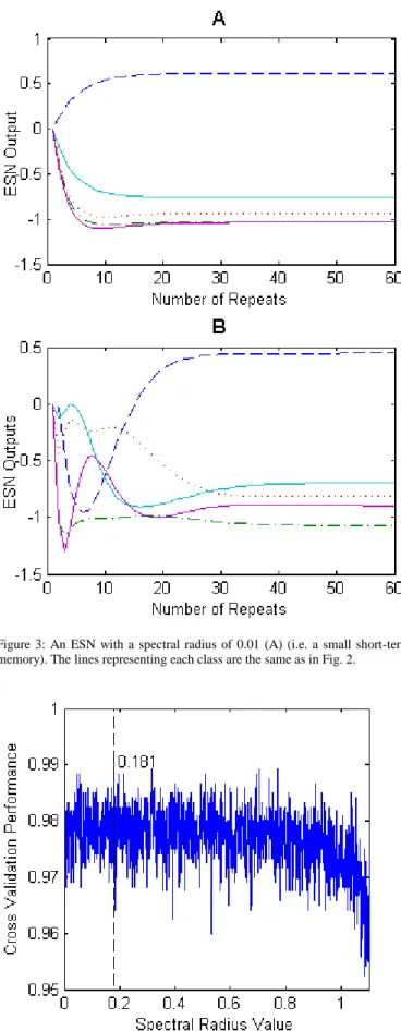
W
'
resres, which represents the initial reservoir weights. Fig. 3 shows the output of two ESNs processing the same clamped input pattern, but with different spectral radii: 0.99 in 3A and 0.01 in 3B. Comparing the plots in Fig. 3A and B, it is clear that the number of repeated input pattern presentations required for the output unit activations to settle is similar, if slightly longer for the smaller spectral radius. Prior to that point, though, the behaviour of the output units is significantly influenced by the network’s memory of previous inputs. When the spectral radius was increased past a value of one, chaotic outputs and poor network classification performance were observed. Based on classification accuracy during the cross-validation testing, the best value for the spectral radius was found to be quite low at 0.181. This suggests that for static classification tasks, a network should be strongly driven by the clamped input pattern, and that reservoir feedback is less important. Consequently, it is better to use a network with more stable dynamics. Importantly, it should be noted that that some feedback is required (i.e. the best spectral radius was greater than zero and performance was generally good for all spectral radii less than one, as can be seen by the range of spectral radii evaluated in Fig. 4). A non-zero spectral radius is therefore one of the properties of the ESN that is desirable for a static pattern classification task.2.1.4 Input Scaling
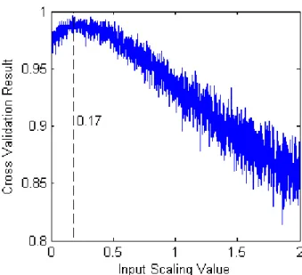
Fig. 5 shows how the performance of the ESN varied as input scaling was varied. When smoothed over 100 points, the results in Fig. 5 can be expressed as a third order polynomial of the form 0.0321s3 - 0.1149s2 + 0.0413s + 0.9825 (R2 = 0.9987), where s is the value of the input scaling. Classification performance during cross-validation peaked with an input scaling value of 0.17. Generally for ESNs, the lower the input scaling value, the more the reservoir units act around the zero point of their hyperbolic tangent (tanh) activation functions. This means that the reservoir units would have been operating in the linear part of the tanh curve.
2.1.5 Interaction between reservoir and output neurons
One of the most instructive details found during the optimization process concerned an important relationship involving the interaction of the ESNs’ reservoir neurons and their output neurons. Compared to the work of Alexandre et al [1], whose focus was on reservoir behaviour, Fig. 6A shows the outputs of twelve randomly selected reservoir neurons for each presentation of a randomly chosen clamped input pattern that was clamped at the input units. Fig. 6B shows the corresponding output activations from each of the five output units during the same input pattern clamping. The vertical dashed line on each plot marks the point
at which output units and the selected reservoir units had plateaued, respectively. The lag between the number of pattern presentations for the reservoir and the output units to plateau indicates that the best results may not necessarily achieved by harvesting values after reservoir stabilisation, as suggested by Alexandre et al [1], but after output unit stabilisation has occurred instead. Furthermore, although the output unit activations had all plateaued after around 24 input pattern presentations during training, the best cross validation classification results were obtained with 60 input pattern presentations, suggesting that the output weights of the ESN need to be trained on a settled reservoir. However, only 24 input pattern presentations are required when a trained network is presented with unseen test data.
2.1.6 Input clamping
Earlier work has noted that reservoir neurons need to be ‘clamped’ until full reservoir stabilisation has been achieved for good classification performance [1–4]. However, while a grid search found that using 60 repeated input pattern presentations (i.e. the same clamping period that was used with the training data) was optimal, it was observed that quite good performance could also be achieved by as few as two input pattern presentations during both the training and testing period. Using only two input presentations is equivalent to obtaining an output without allowing the reservoir to settle at all, suggesting that for good (if not optimal) performance, input ‘clamping’ may be almost unnecessary. This is a counter-intuitive result that goes against the conventional wisdom.
Interestingly, the fact that the reservoir is still in an unstable state for the first ten input presentations means that the number of input presentations in testing must not exceed that used in training, unless the number used in training is greater than the extent of the unstable state. Fig. 7 shows how the output from each node varied with each repeated input pattern. The purple line represents the cherry laurel output node, which should give the highest output value for this test pattern in question. This plot demonstrates why it is important that the number of testing repetitions should not exceed the number of training repetitions when using this approach. Although the cherry laurel node has the highest output after the second presentation, beyond this point a different output node starts to produce much higher values, causing that to become the winner after 25 testing presentations were used. It was usually the case that for every sample presented during testing, each ESN trained on two presentations had one output node consistently produce much higher output values than all of the others, although this was not necessarily the correct winning output node. It seems to be the case that the dynamics of the reservoir and corresponding output weights of the network had been tuned so that the correct output was obtained after the first two presentations, but these weights were not configured to continue produce the correct output when the reservoir dynamics were driven beyond this number of presentations, possibly due to the short term memory of the network.
above. ESNs subject to the first training regime (henceforth referred to as ESN-Op) were presented with the optimal 60 input repeats during both training and testing, while ESNs subject to the second training regime (henceforth referred to as ESN-2R) were given two input repeats during training and testing. By doing this, it would be possible to determine exactly how necessary reservoir stabilisation is for good performance.
3. RESULTS
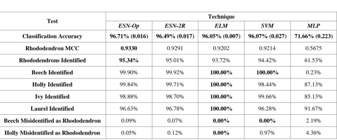
Table 1 gives the performance of each technique on the benchmark datasets. These results show that on average, both ESN architectures achieved better performance than all of the other classifiers, with the exception of the MLP. This confirms that the input clamping methodology can provide good performance when compared to other widely-used classifiers.
As shown in Table 2, the two ESN training regimes used here, ESN-Op and ESN-2R, both produce good test data classification performance comparable to the very widely used ELM and SVM techniques. The MLP, in contrast, was the worst performing technique in all but one category. While it was adept at dealing with the relatively straightforward benchmark datasets, the more challenging real-world dataset proved to be too complex for the MLP. The ELM proved to be the best at distinguishing between non-rhododendron samples, having achieved perfect classification for these during testing. Despite this, the two ESNs were found to be better at correctly identifying rhododendron samples and also gave slightly better overall classification accuracy. The SVM produced good results, but was outperformed by both ESN training regimes in all but three categories. Given that the focus of this task was on detecting rhododendron and that, although they did not classify the other species perfectly, the ESNs misclassified very few of the non-rhododendron samples as false positives, the ESNs offered the best performance of the computational intelligence techniques used for this particular problem.
Curiously, the SVM and ELM gave very similar overall performance, with the SVM proving to be marginally better at rhododendron detection, but with the ELM superior at classifying the other plant species. It would seem that while other classifiers can offer good performance, the recurrent reservoir in an ESN adds certain discriminatory advantages that are not available to other methods.
4. DISCUSSION
Looking at the difference between ESN-Op and ESN-2R, it would appear that there is very little difference between the two techniques in terms of the overall accuracy. ESN-Op marginally outperformed ESN-2R on seven out of the eleven performance measures, including the critical classification accuracy, percentage of rhododendrons identified and rhododendron MCC measures. This difference was, however, found to be insignificant at a 5% significance level using a two tailed t-test. So long as the number of repeated input pattern presentations used during testing is kept the same as the number of clamped presentations
used during training, this t-test result suggests that there is no need to clamp the reservoir neurons until reservoir stabilisation has occurred: contrary to results reported in the literature elsewhere, where it was proposed that the activations of the reservoir units needed to be allowed to settle in order to provide the best ESN performance [1–4]. The most significant contribution of this work, therefore, is that it is possible to obtain accurate results while the reservoir is still unstable, so long as the number of repeated input presentations used during testing is the same as during training. The need for algorithms to determine the point at which the reservoir units can be deemed to have stabilised are thus rendered unnecessary.
5. CONCLUSION
In this paper, ESNs were optimized for static pattern classification and the effect of altering spectral radius, leak rate, input scaling, reservoir size and input pattern repeats on the behaviour of both reservoir and output units was investigated. The performance of these was then tested by presenting them with a challenging classification dataset and comparing them against a standard MLP and very widely used ELMs and SVMs.
Two different ESN training regimes were employed, ESN-2R and ESN-Op, and in each case it was found that the optimized ESNs outperform the widely used classification techniques. Only the MLP produced better classification accuracy on the benchmark datasets, although the MLP later proved incapable of dealing with the more complex leaf sample spectroradiometry dataset. The fact that the ELM and SVM achieved very similar performance implies that the recurrent connections within the reservoir are important for providing optimal classification performance, as does the fact that the optimal ESN spectral radius was greater than zero. The literature regarding the use of ESNs for static pattern recognition suggests that it is necessary to allow the reservoir to settle into a stable state, by ‘clamping’ the input patterns. However, it was found that it is possible to obtain similar classification capability by presenting the input pattern only twice, even though the ESN reservoir might still be in a highly unstable state at this stage, a contribution that defies the conventional wisdom. This idiosyncratic network behaviour needs further investigation, in particular how the spectral radius affects final output designations and the function of the unusually small reservoir. Further work will look into the importance of the reservoir and short term memory for classification ability.
6. ACKNOWLEDGEMENTS
The authors thank NERC FSF for the provision of an equipment grant to S. L. Taylor, which was used to capture the original leaf sample spectroradiometry dataset.
7. COMPLIANCE WITH ETHICAL STANDARDS
Funding: S. L. Taylor has received a research grant from NERC FSF, which was used to capture the original leaf sample spectroradiometry dataset.
Ethical approval: This article does not contain any studies with human participants or animals performed by any of the authors.
[1] L. A. Alexandre, M. J. Embrechts, and J. Linton, “Benchmarking reservoir computing on time-independent classification tasks,” in International Joint Conference on Neural Networks, 2009. IJCNN 2009., 2009, pp. 89–93.
[2] M. J. Embrechts, L. A. Alexandre, and J. D. Linton, “Reservoir computing for static pattern recognition,” in European Symposium on Artificial Neural Networks (ESANN) 2009, 2009.
[3] C. Emmerich, R. Reinhart, and J. Steil, “Recurrence Enhances the Spatial Encoding of Static Inputs in Reservoir Networks,” in Artificial Neural Networks - ICANN 2010, vol. 6353, K. Diamantaras, W. Duch, and L. Iliadis, Eds. Springer Berlin Heidelberg, 2010, pp. 148–153.
[4] R. F. Reinhart and J. J. Steil, “Attractor-based computation with reservoirs for online learning of inverse kinematics,” in European Symposium on Artificial Neural Networks (ESANN) 2009, 2009.
[5] C. Edwards and S. L. Taylor, “A survey and strategic appraisal of rhododendron invasion and control in woodwood areas in Argyll and Bute,” Perth Conservancy, Forestry Commision Scotland, 2008.
[6] F. Williams, R. Eschen, A. Harris, D. Djeddour, C. Pratt, R. S. Shaw, S. Varia, J. Lamontagne-Godwin, S. E. Thomas, and S. T. Murphy, “The Economic Cost of Invasive Non-Native Species on Great Britain,” CABI, 2010.
[7] M. A. Cho, I. Sobhan, A. K. Skidmore, and J. de Leeuw, “Discriminating species using hyperspectral indices at leaf and canopy scales,” in ISPRS 2008 : Proceedings of the XXI congress: Silk road for information from imagery: the International Society for Photogrammetry and Remote Sensing, 2008, pp.
369–376.
[8] K. S. He, D. Rocchini, M. Neteler, and H. Nagendra, “Benefits of hyperspectral remote sensing for tracking plant invasions,” Diversity and Distributions, vol. 17, no. 3, pp. 381–392, 2011.
[9] S. L. Taylor, R. A. Hill, and C. Edwards, “Characterising invasive non-native Rhododendron ponticum spectra signatures with spectroradiometry in the laboratory and field: Potential for remote mapping,” ISPRS Journal of Photogrammetry and Remote Sensing, vol. 81, no. 0, pp. 70–81, 2013. [10] L. Wang, “Invasive species spread mapping using multi-resolution remote sensing data,” The International Archives of the Photogrammetry, Remote
Sensing and Spatial Information Sciences, vol. 37, pp. 135–142, 2008.
[11] R. Gaulton, G. Olaya, E. D. Wallington, and T. J. Malthus, “Continuous Cover Forestry Sensing in the UK? Quantifying Forest Structure using Remote Sensing,” in Proceedings of ForestSAT Conference, 2005.
[12] H. Jaeger, “The ‘echo state’ approach to analysing and training recurrent neural networks,” Fraunhofer Institute for Autonomous Intelligent Systems, 2001.
[13] T. Natschlager, W. Maass, and H. Markram, “The ‘Liquid Computer’: A Novel Strategy for Real-Time Computing on Time Series,” Special Issue on Foundations of Information Processing of TELEMATIK, vol. 8, no. 1, pp. 39–43, 2002.
[14] D. Verstraeten, B. Schrauwen, M. D’Haene, and D. Stroobandt, “An experimental unification of reservoir computing methods,” Neural Networks, vol. 20, no. 3, pp. 391–403, 2007.
[15] L. Busing, B. Schrauwen, and R. Legenstein, “Connectivity, Dynamics, and Memory in Reservoir Computing with Binary and Analog Neurons,” Neural Computation, vol. 22, no. 5, pp. 1272–1311, May 2010.
[16] S. Scardapane and A. Uncini, “Semi-supervised Echo State Networks for Audio Classification,” Cognitive Computation, pp. 1–11, 2016. [17] B. Bacic, “Echo State Network for 3D Motion Pattern Indexing: A Case Study on Tennis Forehands,” in Image and Video Technology: 7th Pacific-Rim
Symposium, PSIVT 2015, Auckland, New Zealand, November 25-27, 2015, Revised Selected Papers, T. Braunl, B. McCane, M. Rivera, and X. Yu, Eds. Cham: Springer International Publishing, 2016, pp. 295–306.
[18] J. B. Butcher, C. R. Day, P. W. Haycock, D. Verstraeten, and B. Schrauwen, “Defect Detection in Reinforced Concrete using Random Neural Architectures,” Computer-Aided Civil and Infrastructure Engineering, vol. 29, no. 3, pp. 191–207, 2014.
[19] A. J. Wootton, C. R. Day, and P. W. Haycock, “Echo State Network Applications in Structrual Health Monitoring,” in Proceedings of the 53rd Annual Conference of The British Institute of Non-Destructive Testing (NDT 2014), 2014, pp. 289–300.
[20] B. Meftah, O. Lezoray, and A. Benyettou, “Novel Approach Using Echo State Networks for Microscopic Cellular Image Segmentation,” Cognitive Computation, vol. 8, no. 2, pp. 237–245, 2016.
[21] L. A. Alexandre and M. J. Embrechts, “Reservoir Size, Spectral Radius and Connectivity in Static Classification Problems,” in Artificial Neural Networks - ICANN 2009, vol. 5768, C. Alippi, M. Polycarpou, C. Panayiotou, and G. Ellinas, Eds. Springer Berlin Heidelberg, 2009, pp. 1015–1024.
[22] G.-B. Huang, Q.-Y. Zhu, and C.-K. Siew, “Extreme learning machine: a new learning scheme of feedforward neural networks,” in Neural Networks, 2004. Proceedings. 2004 IEEE International Joint Conference on, 2004, vol. 2, pp. 985–990 vol.2.
[23] C.-C. Chang and C.-J. Lin, “LIBSVM: A library for support vector machines,” ACM Transactions on Intelligent Systems and Technology, vol. 2, no. 3, pp. 27:1–27:27, 2011.
[24] B. W. Matthews, “Comparison of the predicted and observed secondary structure of T4 phage lysozyme,” Biochimica et Biophysica Acta (BBA) - Protein Structure, vol. 405, no. 2, pp. 442–451, 1975.
[25] K. Bache and M. Lichman, “UCI Machine Learning Repository.” University of California, Irvine, School of Information and Computer Sciences, 2013. [26] X. Dutoit, B. Schrauwen, J. V. Campenhout, D. Stroobandt, H. V. Brussel, and M. Nuttin, “Pruning and regularization in reservoir computing,”
Neurocomputing, vol. 72, no. 7–9, pp. 1534–1546, 2009.
[27] A. E. Hoerl and R. W. Kennard, “Ridge Regression: Biased Estimation for Nonorthogonal Problems,” Technometrics, vol. 12, no. 1, pp. 55–67, 1970. [28] D. C. Montgomery, E. A. Peck, and C. G. Vining, Introduction to Linear Regression Analysis. Wiley, 1982.
[29] M. Lukosevicius, “A practical guide to applying echo state networks,” in Neural Networks: Tricks of the Trade, 2nd ed., vol. 7700, G. Montavon, G. B. Orr, and K.-R. Muller, Eds. Springer Berlin Heidelberg, 2012, pp. 659–686.
[30] H. Jaeger, “A tutorial on training recurrent neural networks, covering BPPT, RTRL, EKF and the ‘echo state network’ approach,” Fraunhofer Institute for Autonomous Intelligent Systems (AIS), 4, 2013.
[31] H. O. Sillin, R. Aguilera, H.-H. Shieh, A. V. Avizienis, M. Aono, A. Z. Stieg, and J. K. Gimzewski, “A theoretical and experimental study of neuromorphic atomic switch networks for reservoir computing,” Nanotechnology, vol. 24, no. 38, p. 384004, 2013.
[32] L. Bozhkov, P. Koprinkova-Hristova, and P. Georgieva, “Reservoir computing for emotion valence discrimination from EEG signals,” Neurocomputing, vol. 231, pp. 28–40, 2017.
[33] M. H. Tong, A. D. Bickett, E. M. Christiansen, and G. W. Cottrell, “Learning grammatical structure with Echo State Networks,” Neural Networks, vol. 20, no. 3, pp. 424–432, 2007.
9. TABLES
Technique Dataset Classification Accuracy
Iris WDBC Average ESN-Op 96.37% 95.17% 95.77% ESN-2R 97.69% 94.90% 96.30% ELM 91.20% 99.96% 95.58% SVM 94.67% 92.75% 93.71% MLP 98.63% 95.99% 97.31%
Table 1: Benchmark dataset results
Test Technique
ESN-Op ESN-2R ELM SVM MLP
Classification Accuracy 96.71% (0.016) 96.49% (0.017) 96.05% (0.007) 96.07% (0.027) 71.66% (0.223) Rhododendron MCC 0.9330 0.9291 0.9202 0.9214 0.5675 Rhododendrons Identified 95.34% 95.01% 93.72% 94.42% 61.53% Beech Identified 99.90% 99.92% 100.00% 100.00% 0.23% Holly Identified 99.84% 99.71% 100.00% 98.44% 87.13% Ivy Identified 98.88% 98.70% 100.00% 99.66% 85.13% Laurel Identified 96.63% 96.78% 100.00% 96.28% 91.67% Beech Misidentified as Rhododendron 0.09% 0.07% 0.00% 0.00% 2.19%
Ivy Misdentified as Rhododendron 0.91% 0.95% 0.00% 0.24% 8.53% Laurel Misidentified as Rhododendron 3.01% 2.82% 0.00% 3.09% 2.30%
10. FIGURES
Figure 1: A typical ESN topology. The input units (left) are fully connected to the reservoir neurons via randomly weighted connections set at initialization. The reservoir is sparsely interconnected with randomly weighted connections and there is potential for recurrent loops. Each reservoir node is connected to each output node (right) and these connections are the only ones that are trained.
Figure 2: ESN outputs over 400 input pattern presentations for the same set of input data. Each coloured line represents values produced by a different output node, with each node representing a different class. The ESN in A has a very low leak rate (0.1) and hence the output varies for some time as the repeats progress, while the ESN in B has a high leak rate (0.9) and thus very fast dynamics. While the output of most units is roughly the same in both cases, the holly output unit settles on a much lower output of -0.7, rather than -0.4. Note also that in 2B, it can be difficult to distinguish between the rhododendron and laurel outputs, which give very similar values.
Figure 3: An ESN with a spectral radius of 0.01 (A) (i.e. a small short-term memory) and an ESN with a spectral radius of 0.99 (B) (i.e. a long short-term memory). The lines representing each class are the same as in Fig. 2.
Figure 6: The activations of twelve randomly selected reservoir neurons (A) and the corresponding outputs of the five output units (B). On each graph, the point at which the data had all plateaued is marked with a dashed line.
Figure 7: The effect of presenting more than two presentations to a network trained on only two presentations. The lines representing each class are the same as in Fig. 6.