Statistical Learning Methods for Personalized Medicine

(1)

Xin Qiu

Submitted in partial fulfillment of the requirements for the degree

of Doctor of Philosophy under the Executive Committee of the Graduate School of Arts and Sciences

COLUMBIA UNIVERSITY

(2)

(3)

Statistical Learning Methods for Personalized Medicine

Xin Qiu

The theme of this dissertation is to develop simple and interpretable individualized treatment rules (ITRs) using statistical learning methods to assist personalized decision making in clinical prac-tice. Considerable heterogeneity in treatment response is observed among individuals with mental disorders. Administering an individualized treatment rule according to patient-specific character-istics offers an opportunity to tailor treatment strategies to improve response. Black-box machine learning methods for estimating ITRs may produce treatment rules that have optimal benefit but lack transparency and interpretability. Barriers to implementing personalized treatments in clin-ical psychiatry include a lack of evidence-based, clinclin-ically interpretable, individualized treatment rules, a lack of diagnostic measure to evaluate candidate ITRs, a lack of power to detect treatment modifiers from a single study, and a lack of reproducibility of treatment rules estimated from single studies. This dissertation contains three parts to tackle these barriers: (1) methods to estimate the best linear ITR with guaranteed performance among the class of linear rules; (2) a tree-based method to improve the performance of a linear ITR fitted from the overall sample and identify subgroups with a large benefit; and (3) an integrative learning combining information across trials to provide an integrative ITR with improved efficiency and reproducibility.

In the first part of the dissertation, we propose a machine learning method to estimate optimal linear individualized treatment rules for data collected from single stage randomized controlled trials (RCTs). In clinical practice, an informative and practically useful treatment rule should be simple and transparent. However, because simple rules are likely to be far from optimal, effective methods to construct such rules must guarantee performance, in terms of yielding the best clinical outcome (highest reward) among the class of simple rules under consideration. Furthermore, it is important to evaluate the benefit of the derived rules on the whole sample and in pre-specified

(4)

maximization, referred to as the asymptotically best linear O-learning (ABLO), which estimates a linear treatment rule that is guaranteed to achieve optimal reward among the class of all linear rules. We then develop a diagnostic measure and inference procedure to evaluate the benefit of the obtained rule and compare it with the rules estimated by other methods. We provide theo-retical justification for the proposed method and its inference procedure, and we demonstrate via simulations its superior performance when compared to existing methods. Lastly, we apply the proposed method to the Sequenced Treatment Alternatives to Relieve Depression (STAR*D) trial on major depressive disorder (MDD) and show that the estimated optimal linear rule provides a large benefit for mildly depressed and severely depressed patients but manifests a lack-of-fit for moderately depressed patients.

The second part of the dissertation is motivated by the results of real data analysis in the first part, where the global linear rule estimated by ABLO from the overall sample performs inadequately on the subgroup of moderately depressed patients. Therefore, we aim to derive a simple and interpretable piece-wise linear ITR to maintain certain optimality that leads to improved benefit in subgroups of patients, as well as the overall sample. In this work, we propose a tree-based robust learning method to estimate optimal piece-wise linear ITRs and identify subgroups of patients with a large benefit. We achieve these goals by simultaneously identifying qualitative and quantitative interactions through a tree model, referred to as the composite interaction tree (CITree). We show that it has improved performance compared to existing methods on both overall sample and subgroups via extensive simulation studies. Lastly, we fit CITree to Research Evaluating the Value of Augmenting Medication with Psychotherapy (REVAMP) trial for treating major depressive disorders, where we identified both qualitative and quantitative interactions and subgroups of patients with a large benefit.

The third part deals with the difficulties in the low power of identifying ITRs and replicating ITRs due to small sample sizes of single randomized controlled trials. In this work, a novel inte-grative learning method is developed to synthesize evidence across trials and provide an inteinte-grative ITR that improves efficiency and reproducibility. Our method does not require all studies to collect a common set of variables and thus allows information to be combined from ITRs identified from

(5)

to enhance a high-resolution ITR by borrowing information from coarsened ITRs or improve the coarsened ITR from a high-resolution ITR. With a simple modification, the proposed integrative learning can also be applied to improve the estimation of ITRs for studies with blockwise missing feature variables. We conduct extensive simulation studies to show that our method has improved performance compared to existing methods where only single-trial ITRs are used to learn personal-ized treatment rules. Lastly, we apply the proposed method to RCTs of major depressive disorder and other comorbid mental disorders. We found that by combining information from two studies, the integrated ITR has a greater benefit and improved efficiency compared to single-trial rules or universal non-personalized treatment rule.

Key Words: Personalized medicine; Machine learning; Treatment response heterogeneity; Indi-vidualized treatment rules; Qualitative interaction; Quantitative interaction; Robust loss function; Tree-based method; Integrative learning; Blockwise missing data

(6)

List of Figures iv

List of Tables vi

1 Introduction 1

1.1 Background and Overview . . . 1

1.2 Introduction to Estimation and Evaluation of Linear Individualized Treatment Rules 3 1.3 Introduction to Composite Interaction Tree for Learning Optimal Individualized Treatment Rules and Subgroups . . . 6

1.4 Introduction to Integrative Learning to Synthesize Individualized Treatment Rules Across Multiple Trials . . . 10

2 Estimation and Evaluation of Linear Individualized Treatment Rules to Guar-antee Performance 15 2.1 Overview . . . 15

2.2 Methodologies. . . 16

2.2.1 Estimating Optimal Linear Treatment Rule . . . 17

2.2.2 Performance Diagnostics for the Estimated ITR. . . 21

(7)

2.4 Simulation Studies . . . 30

2.4.1 Simulation Design . . . 30

2.4.2 Simulation Results . . . 33

2.5 Application to the STAR*D Study . . . 35

2.6 Discussion . . . 38

3 Composite Interaction Tree for Learning Optimal Individualized Treatment Rules and Subgroups 46 3.1 Overview . . . 46 3.2 Methodologies. . . 47 3.3 Simulation Studies . . . 52 3.3.1 Simulation Study 1 . . . 53 3.3.2 Simulation Study 2 . . . 57

3.4 Application to the REVAMP Study . . . 63

4 Integrative Learning to Synthesize Individualized Treatment Rules Across Mul-tiple Trials 74 4.1 Overview . . . 74

4.2 Methodologies. . . 75

4.2.1 Integrative Learning for High-Resolution ITR Using Coarsened ITRs . . . 75

4.2.2 Integrative Learning for Coarsened ITRs Using High-Resolution ITR . . . 78

(8)

4.4 Simulations . . . 83

4.4.1 Simulation Design . . . 83

4.4.2 Simulation Results . . . 85

4.5 Application to the EMBARC trial . . . 89

Bibliography 96 A Appendices for Chapter 2 106 A.1 Computing the Theoretical Optimal Linear Rule . . . 106

A.2 Additional Simulation Results. . . 108

A.3 Sensitivity to the Starting Values of ABLO . . . 108

B Appendices for Chapter 3 114 B.1 Estimation of Variance forbδC1(fb)−bδC2(fb) . . . 114

C Appendices for Chapter 4 118 C.1 Simulation Study for Multiple Trials with Different Treatment Effects . . . 118

(9)

1.1 Three types of covariates (prognostic, predictive and prescriptive). . . 2

2.1 Different approximation functions of the zero-one loss . . . 18

2.2 Clinical outcome (R) versus W with treatment 1 or −1 in each latent group in the

simulation setting. Two vertical dotted lines indicate W =−0.5 andW = 0.5.. . . . 32

2.3 Simulation results: Overall ITR benefit and optimal treatment accuracy rates for

the four methods . . . 40

2.4 Simulation results: Subgroup ITR benefit for the four methods . . . 43

2.5 STAR*D analysis results: Distribution of the estimated ITR benefit (the higher the

better) and QIDS score (the lower the better) at the end of level-2 treatment for the

four methods (based on 500 cross-validation runs). . . 45

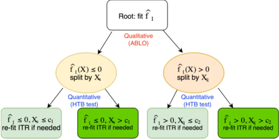
3.1 Diagram of an example Composite Interaction Tree (CITree)∗ . . . 48

3.2 CITree structure for generating data of simulation studies (left panel: simulation

study 1; right panel: simulation study 2) . . . 54

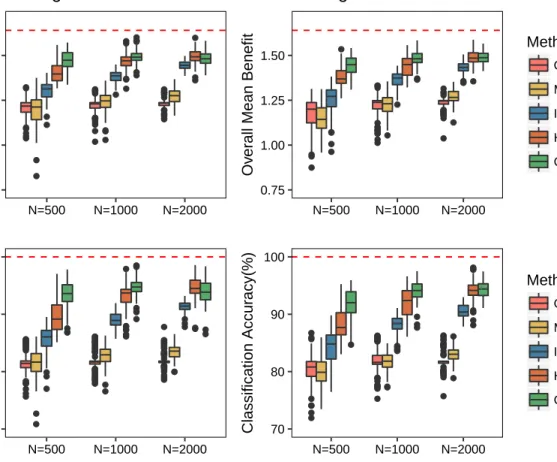
3.3 Overall performance of five methods in simulation study 2 . . . 59

3.4 Simulation 2 results for subjects in terminal nodes T1, T2, and T5∗ . . . 69

(10)

3.7 CITree for optimal individualized treatment decision (the REVAMP Study) . . . 73

4.1 An example for data collected with blockwise feature domains . . . 80

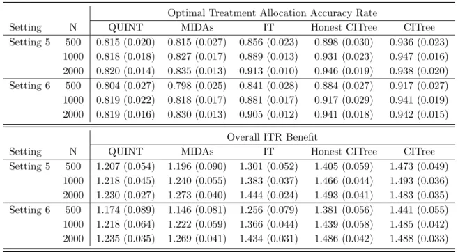
4.2 Overall ITR benefit and optimal treatment allocation accuracy for the four methods. 87

4.3 Overall ITR benefit and optimal treatment allocation accuracy for the three methods. 89

4.4 Overall performance of the four methods in EMBARC study using HEAL ITR . . . 92

4.5 Overall performance of the four methods to handle blockwise feature domain data

in EMBARC study . . . 93

A.1 Simulation results: Overall ITR benefit and accuracy rates for the four methods . . 111

A.2 Simulation results: Subgroup ITR benefit for the four methods . . . 112

A.3 Performance of the algorithm on two example datasets evaluated by value function

and penalized weighted sum of ramp loss. . . 113

C.1 Overall ITR benefit and optimal treatment allocation accuracy for the four methods 120

C.2 Overall ITR benefit and optimal treatment allocation accuracy for the three methods.121

(11)

2.1 Simulation results: mean and standard deviation of the accuracy rate, mean ITR

benefit, and coverage probability for estimation of the benefit of the optimal ITR . . 41

2.2 Simulation results: probability of rejecting the null hypothesis that the treatment benefit across subgroups is equivalent by the HTB test . . . 42

2.3 Simulation results: Comparison of the ITR to the non-personalized universal rule. The proportion of rejecting the null that the ITR has the same benefit as the universal rule∗ are reported for the overall sample and by subgroups. . . 44

2.4 Results of STAR*D Data Analysis . . . 45

3.1 Simulation study 1 results: type I error rate and power for HTB tests . . . 56

3.2 Simulation study 2 results: comparing overall performance of five methods . . . 60

3.3 Simulation study 2 results: classification accuracy among subjects truly belong to each terminal node . . . 68

3.4 Simulation study 2 results: total nodes or levels of tree based methods . . . 71

3.5 Simulation study 2 results: PPVs of predicted terminal nodes by CITree . . . 71

3.6 Simulation study 2 results: subgroup benefits of predicted terminal nodes by CITree 72 3.7 Overall performance of three methods in the REVAMP Study . . . 73

(12)

studies . . . 86

4.2 Mean and standard deviation of overall benefit, value and accuracy rates using

in-tegrative learning for low-resolution ITRs comparing to ITRs by ABLO on single

studies . . . 88

4.3 Overall performance of the four methods in EMBARC study using HEAL ITR . . . 92

4.4 Overall performance of the four methods to handle blockwise feature domain data

in EMBARC study . . . 93

A.1 Simulation results: mean and standard deviation of the accuracy rate, mean benefit,

and coverage probability for estimation of the benefit of the optimal ITR . . . 110

C.1 Mean and standard deviation of overall benefit, value and accuracy rates for integra-tive learning of high-resolution ITR comparing to ITRs by ABLO on single studies

. . . 120

C.2 Mean and standard deviation of overall benefit, value and accuracy rates for integra-tive learning of low-resolution ITR comparing to ITRs by ABLO on single studies

. . . 121

(13)

Foremost, I would like to express my deepest gratitude to my advisor, Professor Yuanjia Wang, for her invaluable guidance and constant support during the past four years. I could not have come this far without her motivation, encouragement, and trust in my abilities. During our weekly meeting, Professor Wang always gave me inspiring advice and insightful feedback to facilitate my research. I am very lucky and grateful to work with her for the past few years as a PhD student and research assistant. A special thanks goes to Professor Donglin Zeng, for providing invaluable suggestions and insightful comments to improve my work from the beginning of thesis proposal to the end of defense.

I would also like to express my sincere gratitude to my dissertation committee members, Pro-fessor Bruce Levin, ProPro-fessor Bin Cheng, ProPro-fessor Gen Li, and ProPro-fessor Eva Petkova, who offered helpful feedback and inspiring questions to perfect this dissertation. And I would like to thank Pro-fessor Christine Mauro and ProPro-fessor Katherine Shear for supervising my research assistantship.

I would like to thank the Department of Biostatistics for providing me fellowship. I wish to acknowledge all the faculty and staff in the department. In particular, I wish to thank all my classmates for sharing this journey together.

Last but not the least, I would like to thank my family and friends for their unconditional love and support.

(14)

(15)

Chapter 1

Introduction

1.1 Background and Overview

Heterogeneity in patient response to treatment is a long-recognized challenge in the clinical

com-munity. For example, in adults affected by major depression, only around 30% of patients achieve

remission with a single acute phase of treatment (Trivedi et al., 2006; Rush et al., 2004); the

remaining 70% of patients require augmentation of the current treatment or a switch to a new

treatment (Trivedi and Daly, 2008). Heterogeneity in treatment response also has been observed

among children with attention deficit and hyperactivity disorder (Pelham and Fabiano,2008), and

autism spectrum disorders (Jones et al.,2010). Thus, a universal strategy that treats all patients

with the same treatment is inadequate, and individualized treatment strategies are required to

im-prove response in individual patients. In this regard, rapid advances in technologies for collecting

patient-level data have made it possible to tailor treatments to individual patients based on their

characteristics, thereby enabling the new paradigm of personalized medicine.

(16)

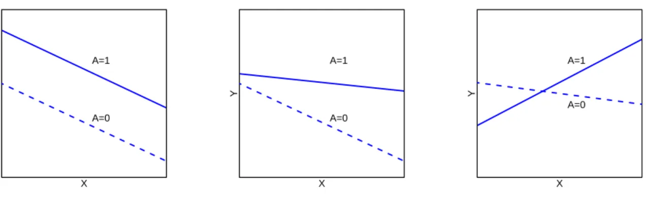
Figure 1.1: Three types of covariates (prognostic, predictive and prescriptive) No interaction X Y A=1 A=0 Quantitative interaction X Y A=1 A=0 Qualitative interaction X Y A=1 A=0

at the right time, in order to improve patient care and reduce potential side effects and health

care cost (Carini et al., 2014). As depicted in Figure 1.1, three types of patient’s covariates may

be considered to achieve this goal. The first class of covariates includes prognostic variables which

inform selecting subgroups of subjects at high risk for disease, irrespective of the treatment they

receive (Carini et al., 2014). The other two classes of covariates correspond to variables with

either quantitative or qualitative interaction with treatments, which are referred as predictive or

prescriptive variables, respectively. In particular, qualitative interaction refers to that the treatment

effect changes direction based on some function of covariates, which indicates that a treatment could

be superior in one subgroup but inferior in another subgroup. This type of interaction provides

important information on estimating a personalized treatment rule. Quantitative interaction refers

to that the treatment effects are in the same direction in the covariate space but differ in magnitude

in some subgroup. Predictive variables manifest quantitative interaction and define subgroups of

subjects who are likely to experience large treatment benefit, while prescriptive variables manifest

(17)

variables can be used to guide the development of personalized medicine (Carini et al.,2014).

In the following of this dissertation, we develop several new statistical learning methods for

estimating simple and interpretable individualized treatment rules for single-stage randomized

con-trolled trials. The dissertation consists of three projects. We start by introducing background and

motivation of each project. In Chapter 2, we propose a machine learning method to estimate the

optimal linear individualized treatment rule and a diagnostic measure to assess the optimality of

candidate rules. In Chapter 3, we improve the performance of a linear ITR fitted from the

over-all sample using a tree-based model to identify both qualitative and quantitative interactions and

subgroups of subjects with a large benefit. In Chapter4, we use integrative learning to synthesize

evidence across multiple trials to improve efficiency and reproducibility of the estimation of ITRs.

1.2 Introduction to Estimation and Evaluation of Linear

Individ-ualized Treatment Rules

Statistical methods have been proposed to estimate optimal individualized treatment rules (ITRs)

(Lavori and Dawson,2004) using predictive and prescriptive clinical variables that manifest

quanti-tative and qualiquanti-tative treatment interactions, respectively (Carini et al.,2014;Gunter et al.,2011).

Q-learning (Watkins,1989; Qian and Murphy,2011) and A-learning (Murphy, 2003;Blatt et al.,

2004) are proposed to identify the optimal ITR. Q-learning is a regression-based method, which

esti-mates an ITR by directly modeling the Q-function (“Q” stands for “quality of action”). A-learning

only requires posited models for contrast functions and uses a doubly robust estimating equation

to estimate the contrast functions. This makes A-learning more robust to model misspecification

(18)

pro-posed approaches include semiparametric methods and machine learning methods (Moodie et al.,

2007; Zhang et al., 2012; Foster et al., 2011; Zhao et al., 2012; Chakraborty and Moodie, 2013).

For example, the virtual twins approach (Foster et al.,2011) uses tree-based estimators to identify

subgroups of patients who show larger than expected treatment effects. Zhang et al. (2012,2013)

estimated the optimal ITR by directly maximizing the value function over a specified parametric

class of treatment rules through augmented inverse probability weighting. In contrast, Zhao et al.

(2012) proposed outcome weighted learning (O-learning), which utilizes weighted support vector

machine to directly maximize the value function (expected clinical outcome by following the ITR).

More recently, Huang and Fong (2014) proposed a robust machine learning method to select the

ITR that minimizes a total burden score due to disease and treatment for a binary clinical outcome.

Interactive Q-learning (Laber et al.,2014) models two ordinary mean-variance functions instead of

modeling the predicted future optimal outcomes. Fan et al.(2017) proposed a concordance function

for prescribing treatment, where a patient is more likely to be assigned to a treatment than another

patient if s/he has a greater benefit than the other patient.

In clinical practice, simple treatment rules such as linear rules, are preferred due to their

trans-parency and convenience for interpretation. However, when only linear rules are in consideration,

many existing methods including semiparametric models and some machine learning methods may

not yield a rule with optimal performance, because they focus on optimization of a surrogate

ob-jective function of treatment benefit. Using surrogate obob-jective functions may only guarantee the

optimality when there is no restriction on the functional form of the treatment rules. For

exam-ple, with O-learning, the objective function is a weighted hinge-loss, which yields the optimal rule

among nonparametric rules, but may not be optimal when the candidate rules are restricted to the

(19)

performance when constraints are placed on the class of candidate rules.

An additional consideration is the need to evaluate, through diagnostics, any approach for rule

estimation. However, less emphasis has been placed on the evaluation of the estimated ITR in the

context of personalized medicine. Residual plots were used to evaluate model fit for G-estimation

(Rich et al., 2010) and Q-learning (Ertefaie et al., 2016). In the recent work by Wallace et al.

(2016), a dynamic treatment regime (DTR) is estimated by G-estimation and double robustness

is exploited for model diagnosis. How to evaluate the optimality of an ITR in general remains an

open research question.

The purpose of this work is two-fold: we first develop a general approach to identify a linear ITR

with guaranteed performance; we then propose a diagnostic method to evaluate the performance

of any derived ITR including the proposed one. Our two-stage approach separates the estimation

of the ITR from its evaluation and the sample used in each stage. Specifically, in the first stage,

we propose ramp-loss-based (McAllester and Keshet,2011;Huang and Fong,2014) learning for the

estimation and we show that this approach guarantees the derived linear ITR to be asymptotically

optimal within the class of all linear rules. We refer our method as Asymptotically Best Linear

O-learning, ABLO. For the second stage, in practice, it is infeasible to expect that an ITR that benefits

each individual can be identified due to the unknown treatment mechanism and the likely omission

of some prescriptive variables. Thus, we propose a practical solution to calibrate the average ITR

effect in the population given the observed variables, or in pre-specified important subgroups (e.g.,

patients in the most severe state). Specifically, to obtain an ITR evaluation criterion, we define the

benefit of a candidate ITR as the average difference in the value function between those who follow

the ITR and those who do not. We then use the ITR benefit as a diagnostic measure to evaluate

(20)

for any given patient subgroup, the average outcome for patients who are treated according to the

ITR should be greater than for those who are not treated according to the ITR. On the contrary,

if the average outcome of the ITR is worse for some patients who follow the ITR than for those

who do not, then the ITR is not optimal on this subgroup.

Compared to the existing literature, two main contributions of this work are to propose a benefit

function to calibrate an ITR, and a diagnostic procedure to evaluate optimality of a derived ITR,

while most of the existing work focuses on the estimation of ITR/DTR. A third contribution is

to prove asymptotic properties of ITR estimated under the ramp loss (Huang and Fong, 2014).

Asymptotic results in the existing literature (e.g., Zhao et al. (2012)) are obtained for the hinge

loss. Due to these theoretical results, we can provide valid statistical inference procedure for testing

optimality of an ITR using asymptotic normality.

In Chapter 2, we show that ABLO consistently estimates the ITR benefit for a class of

candi-date rules regardless of two potential pitfalls: 1) the consistency of benefit estimator is maintained

even though the functional form of the rule is misspecified; 2) the rule does not include all

pre-scriptive/tailoring variables and thus the true global optimal rule is not in the specified class. We

further derive the asymptotic distribution for the proposed diagnostic measure. We conduct

simu-lation studies to demonstrate finite sample performance and show advantages over existing machine

learning methods. Lastly, we apply the method to the Sequenced Treatment Alternatives to Relieve

Depression (STAR*D) trial on major depressive disorder (MDD), where substantial treatment

re-sponse heterogeneity has been documented (Trivedi et al.,2006;Huynh and McIntyre,2008). Our

analyses estimate an optimal linear ITR, and we demonstrate a large benefit in mildly depressed

(21)

1.3 Introduction to Composite Interaction Tree for Learning

Op-timal Individualized Treatment Rules and Subgroups

Due to their simplicity and interpretability, decision trees are often constructed to assist

person-alized medical decision making. Two types of interactions are useful for personalizing treatments:

qualitative interactions inform the selection of optimal treatment from several competing choices;

quantitative interactions inform the identification of subgroups with a substantially greater or

smaller response than the overall sample. Methodologies are proposed to estimate an optimal ITR

by hunting for qualitative interactions between covariates and treatments on the outcome (Carini

et al., 2014; Gunter et al., 2011; Dusseldorp and Van Mechelen, 2014; Laber and Zhao, 2015).

Specifically, Qualitative interaction tree (QUINT,Dusseldorp and Van Mechelen,2014) partitions

patients into terminal nodes where the average effect of one treatment for patients in the nodes is

superior or two treatments are similar. Unlike the usual classification trees or regression trees where

class labels are known, in tree-based methods for estimating optimal ITRs the optimal treatment

(class label) for an individual is unknown. In this regard, Minimum Impurity Decision Assignments

decision trees (MIDAs,Laber and Zhao,2015) focused on the estimation of a tree-structured ITR

that maximizes a value function and splits the parent nodes where the value function will be most

dramatically improved. Fu et al. (2016) proposed to maximize the value function by exhaustive

search; their approach was shown to be more stable due to using residuals of a regression model

to remove main effects of covariates on the outcome when learning a tree (Liu et al.,2014). In a

recent work byZhu et al.(2017), outcome weighted learning (Zhao et al.,2012) and reinforcement

learning tree (Zhu et al.,2015) were combined to construct a tree-based model to perform treatment

(22)

used to evaluate the potential contribution of each variable.

Another group of methods is proposed to identify treatment response heterogeneity through

estimating quantitative interactions. In this case, the optimal treatment may be the same for

a subgroup of patients but they manifest a greater benefit than the overall sample. Subgroup

Identification based on Differential Effect Search (SIDES, Lipkovich et al., 2011) searches within

certain regions of the covariate spaces and identifies multiple subgroups with enhanced treatment

effects. At each step, SIDES partitions a parent node into two child nodes for each covariate in a

pre-specified set and retains the child node with a larger treatment effect. Virtual twins (Foster

et al., 2011) finds a subgroup of patients who will have larger treatment effect using tree-based

estimators. Interaction trees (ITs, Su et al.,2009) can identify both qualitative and quantitative

interaction, but cannot distinguish strong quantitative interaction from qualitative interaction.

Some of the above existing tree-based approaches (e.g., QUINT, IT) examine qualitative

inter-action by exploring each candidate feature variable in turn. However, due to biological and clinical

heterogeneity among patients, a single variable is unlikely to successfully guide treatment choice

in individual patients; information carried by a single variable is limited, and a large number of

variables each with small effects may play a role. Thus, tree-based approaches that partitions by

individual variables may have reduced performance. For instance, in a randomized trial treating

major depressive disorder (STAR*D, Rush et al., 2004), QUINT did not return any individual

variable that can distinguish the best treatment to reduce depressive symptoms. In contrast, using

the same study data, machine learning and regression-based approaches (Chakraborty and Moodie,

2013;Qiu et al., 2017) identified ITRs as linear combinations of feature variables that manifest a

qualitative interaction to differentiate optimal treatments for individual patients. However, a

(23)

subgroups (due to the misspecification of linear rules), and thus do not identify subgroups with

large ITR benefits.

Recognizing that estimating an ITR and identifying subgroups with large ITR benefits are

two important goals, we propose a novel composite interaction tree, referred to as CITree, to

simultaneously estimate qualitative and quantitative interactions. CITree contains two types of

splits: a qualitative-interaction split by fitting asymptotically best linear rule (ABLO) at each

stage; and a quantitative-interaction split based on a heterogeneity of ITR benefit (HTB) test.

Specifically, in the qualitative split CITree estimates an interpretable, simple decision tree that

guarantees enhanced performance on subgroups of patients by improving the value function fitted

from the overall sample. Patients are partitioned into homogeneous subgroups of similar optimal

ITR (reduce optimal treatment rule heterogeneity). In the quantitative split, CITree partitions

patients into homogeneous subgroups of ITR benefit such that the within-group optimal ITR effect

is similar while the between-group difference is large (reduce ITR benefit heterogeneity).

CITree leverages a diagnostic measure of the goodness-of-fit of a decision rule and a measure

of the ITR benefit (i.e., the difference in the mean response for patients who follow the ITR and

those who do not). It has been shown in Chapter 2 that if an optimal ITR genuinely maximizes

the clinical response in each individual patient, then the ITR will have a positive effect within any

arbitrarily defined subgroup of patients. Thus, by an HTB test, it is feasible to determine for which

patients a linear (and potentially misspecified) ITR leads to a significantly lower than average (and

potentially negative) benefit; thus the treatment is more likely to be non-optimal for these patients.

To remedy this lack-of-fit of linear rules, as patients travel down the CITree, non-optimal ITRs with

a poor benefit at top nodes are rectified in subgroups and patients organize into nodes of a high or

(24)

re-fit ITR within the subgroups (qualitative split), CITree will improve the overall value function

and increase the subgroup benefit.

In Chapter 3 of this dissertation, we further introduce the rationale and algorithm of CITree.

We show that CITree can successfully reduce the benefit heterogeneity and rule heterogeneity. We

then perform extensive simulation studies to show improvement as compared to existing machine

learning methods (e.g., IT, QUINT). Lastly, we fit a CITree using the Research Evaluating the

Value of Augmenting Medication with Psychotherapy (REVAMP) trial data for treating major

depressive disorder (MDD), where substantial treatment response heterogeneity was documented

in the literature (Shankman et al.,2013).

1.4 Introduction to Integrative Learning to Synthesize

Individu-alized Treatment Rules Across Multiple Trials

Several challenges hamper the success of developing and implementing personalized treatment

de-cisions in clinics. First, recent machine learning methods (Zhao et al.,2012,2015) for discovering

individualized treatment rules (ITRs) lack interpretability, and thus, they are difficult to

under-stand by clinicians and translate into clinical practice. Second, most randomized controlled trials

(RCTs) are powered to detect average treatment effects instead of subgroup effects, let alone

op-timal individualized treatment decisions. Thus, subgroup or ITR findings are difficult to replicate

due to small sample sizes. Third, the target population for the application of ITRs can be different

from the patient sample used in estimating the ITR due to time, geographic, or other differences

(Justice et al.,1999). When learning an ITR based on a single study, the research aim is to estimate

(25)

to a future sample due to sample difference between studies and the study-specific noise variables.

A cost-effective method to remedy the small sample size problem and improve the reproducibility

and transportability is to pool and analyze data from multiple RCTs, which includes meta-analysis

(Haidich,2010) and integrative analysis approaches (Ma et al.,2011). Meta-analysis uses a weighted

average to compute a pooled estimate of an average overall treatment effect from individual studies

(Cipriani et al.,2018;Jakobsen et al.,2017). Subgroup analyses are exploratory in nature, and

well-designed studies testing the same subgroup effect is scarce in the literature. Therefore, conducting

subgroup meta-analysis across multiple trials is difficult. For example, we performed a systematic

review of subgroup analysis of RCTs of major depressive disorder (MDD). There were 211 studies

that met our inclusion criteria, but with only one consensus predictive variable (i.e., baseline severity

of depression), suggesting that the literature is incomplete and inconclusive given the substantial

observed heterogeneity in treatment effects (HTE). On the other hand, we didn’t find any research

performing meta-analysis for ITRs because there is no straightforward method to average ITRs

from individual studies given that an ITR is usually the sign of a decision function. Integrative

analysis approaches pool raw data from multiple studies and analyze the pooled data as if it is

from a single trial. Integrative analysis can be more effective than meta-analysis (Ma et al.,2011),

and has been used in detecting genetic risk factors from multiple cancer studies or cancer subtypes.

However, it requires that multiple studies share the same biological ground and the same candidate

feature variables should be collected from all the studies.

In practice, due to different study designs and hypotheses, RCTs often collect different sets of

baseline covariates or feature variables. When new evidence from neuroscience research emerges,

new hypotheses are proposed regarding various biomarkers as predictive/prescriptive variables for

(26)

collec-tion, in addition to clinical and neuropsychiatric measures (EMBARC,Trivedi et al.(2016)), while

in prior studies (e.g, STAR*D (Rush et al., 2004), CO-MED (Rush et al., 2011), HEAL (Shear

et al., 2016), REVAMP (Kocsis et al., 2009), Nefazodone-CBASP (Keller et al., 2000), Bulimia

(Sysko et al., 2010)), only comprehensive clinical variables are available. In particular, EMBARC

trial collects comprehensive baseline measures including clinical measures, depression and anxiety

measures, behavioral phenotyping (BP), functional magnetic resonance imaging (fMRI),

electroen-cephalogram (EEG), and diffusion tensor imaging (DTI). In addition to clinical measures,

depres-sion and anxiety measures, STAR*D and Co-Med also include information for measuring quality

of life, work and social adjustment, while HEAL consists of additional variables to measure grief

symptoms and treatment expectancy.

Non-uniform, heterogeneous feature collection poses challenges for the integration of ITRs or

meta-analysis across RCTs. Combining data directly and performing a single analysis is often

inefficient or inappropriate. For example, one may consider to use all subjects with common feature

variables across trials and treat it as a single study, which may lose information of important feature

variables. On the other hand, to include as many feature variables as possible, one may end up

with a small number of subjects in the analysis, which may lead to a biased sample to represent

the entire population.

Because available feature variables in each trial differ, treatment rules estimated from each trial

will include different “resolutions” of the patient-specific characteristics (i.e., ITRs from EMBARC

may depend on both clinical variables and brain imaging biomarkers, whereas ITRs from STAR*D

depend only on clinical variables). The fitted ITRs may yield opposite treatment recommendations

for the same patient based on different feature variables included. A conundrum is that although

(27)

treatment for an individual patient, these ITRs can be less reliable due to an increased number of

tailoring variables. Conversely, coarsened ITRs learned using fewer variables are more robust and

practical in resource-limited clinical settings (e.g., when collecting data on expensive biomarkers

is prohibitive). However, these ITRs may not lead to a truly optimal personalized treatment.

Therefore, integration and reconciliation of the ITRs learned on heterogeneous scales are important.

We will propose novel analytic solutions to the above challenges. Our proposed method is related

to Multi-Task Learning (MTL) and Multi-Objective Reinforcement Learning (MORL). One type of

MTL (Ruder,2017) is to optimize one loss function with related auxiliary tasks to improve the main

task. MORL (Liu et al.,2015) aims to optimize multiple objectives by summarizing them into one

single objective. When multiple studies collecting features with different resolutions are available,

depending on the main study of interest and information available in the future target population

of applying the estimated ITR, other studies can be included as auxiliary data sets to improve

the efficiency and reproducibility of the ITR comparing to using the main study data set alone.

When learning a high-resolution ITR is of interest, the auxiliary data sets often collect a subset

of feature variables which can provide resolution ITRs. If a simple and easy to interpret

low-resolution ITR is of interest, auxiliary data sets with high-low-resolution ITRs can still assist improving

the coarsened ITR based on the low-resolution information.

To improve efficiency and reproducibility of ITRs from both directions, we propose a novel

in-tegrative learning to synthesize evidence across trials and provide an inin-tegrative ITR. Our method

does not require all studies to collect common sets of variables. Thus, the integrative learning allows

evidence to be combined from ITRs identified in recent RCTs that collected emerging biomarkers

(e.g., neuroimaging measures) with earlier RCTs that focused on clinical and psychosocial markers.

(28)

func-tion and use a data-driven method to determine how much evidence each study contributes to the

integrative ITR. Optimization of the regularized value function can be easily solved using existing

outcome-weighted learning methods (Zhao et al.,2012;Qiu et al.,2017) with an augmentation term

related to the clinical outcome.

In Chapter4of this dissertation, we first introduce the rationale and algorithm of the proposed

integrative machine learning method for learning both high-resolution ITRs and coarsened ITRs.

We then extend the proposed method to studies collecting blockwise feature domains. We derive

the underlying Bayesian rules for the proposed method. We show that the proposed method

can successfully improve the efficiency and reproducibility of the estimated ITRs compared to

existing machine learning methods for single studies (e.g., ABLO) via extensive simulation studies.

Lastly, we fit ITRs using the proposed integrative learning method on Establishing Moderators

and Biosignatures of Antidepressant Response in clinical Care (EMBARC) trial for treating major

(29)

Chapter 2

Estimation and Evaluation of Linear

Individualized Treatment Rules to

Guarantee Performance

2.1 Overview

In this chapter, we propose a machine learning method, asymptotically best linear O-learning

(ABLO) to estimate the optimal linear ITR. We also propose a diagnostic measure to evaluate

candidate ITRs. In Section 2.2, we propose the statistical method of ABLO and several tests for

goodness-of-fit. In Section 2.3, we show the asymptotic properties. In Section 2.4, we conduct

simulation studies to investigate the performance of the proposed method. In Section2.5, we apply

the method to a study of patients with major depressive disorder, the STAR*D data. Finally, we

(30)

2.2 Methodologies

We start by introducing some notations for single-stage randomized clinical trials. Let R denote

a continuous variable measuring clinical response after treatment (e.g., reduction of depressive

symptoms). Without loss of generality, assume a large value of R is desirable. Let X denote a

vector of subject-specific baseline feature variables, and letA= 1 orA=−1 denote two alternative

treatments being compared. Assume that we observe (Ai,Xi, Ri) for theith subject in a two-arm

randomized trial with randomization probability P(Ai =a|Xi =x) =π(a|x), for i= 1, ..., n.

An ITR, denoted asD(X), is a binary decision function that mapsX into the treatment domain

A={−1,1}. LetPD denote the distribution of (A,X, R) in whichDis used to assign treatments.

The value function of Dsatisfies

V(D) =ED(R) = Z R dPD= Z R dP D dP dP =E ( RI(A=D(X)) π(A|X) ) , (2.1)

where P is the distribution of (A,X, R) and PD is the distribution under A = D(X). In most

applications, D(X) is determined by the sign of a function,f(X), which is referred to as the ITR

decision function. That is,D(X) = sign(f(X)). In general settings,f ∈ Fcan take any form, either

a parametric function or a non-parametric function. To quantify the benefit of an ITR, a measure

related to the value function is a natural choice. The mean difference is widely used to compare

the average effect of two treatments. Analogously, we define the benefit function corresponding to

an ITR as the difference in the value function between two complementary strategies: one that

assigns treatments according toD(X) and the other assigns according to the complementary rule

−D(X) for any given feature variablesX. That is, the benefit function forD(X) = sign(f(X)) is

(31)

2.2.1 Estimating Optimal Linear Treatment Rule

To obtain a practically useful and transparent ITR, we consider a class of linear ITR decision

functions, denoted by L, and estimate the optimal linear function f_L∗ ∈ L, that maximizes the

value function (2.1) among this class. To this end, following the original idea of Liu et al. (2014),

we note that maximizing V(D) is equivalent to minimizing a residual-weighted misclassification

error given as E |R−r(X)|I{A sign(R−r(X))6=D(X)} π(A|X) ,

where r(X) is any function of X, taken as an approximation to the conditional mean of R given

X. Thus, we aim to minimize the empirical version of the above quantity, given as

1 n X i |Wi|I(AiZi 6=D(Xi)) π(Ai|Xi) = 1 n X i |Wi|I(AiZif(Xi)<0) π(Ai|Xi)

forf ∈ L, whereWi=Ri−br(Xi),Zi = sign(Wi), andbr(X) is obtained from a working model by

regressing Ri onXi (Liu et al.,2014).

The above optimization with zero-one loss is a non-deterministic polynomial-time hard

(NP-hard) problem (Natarajan, 1995). To avoid this computational challenge, the zero-one loss was

replaced by some convex surrogate loss in existing methods, for instance, the squared loss or hinge

loss. Let f∗ denote the global optimal decision function corresponding to the optimal treatment

rule among any decision functions. That is, f∗(X) =E(R|A = 1,X)−E(R|A =−1,X). When

L consists of linear decision functions that are far from the global optimal rule such that f∗ 6∈ L,

estimating optimal linear rule by minimizing the surrogate loss (e.g., hinge loss or squared loss) no

longer guarantees that the induced value or benefit is maximized among the linear class.

In order to obtain the best linear ITR with guaranteed performance, we propose to use an

(32)

(McAllester and Keshet,2011;Huang and Fong,2014), for value maximization. The ramp loss, as

plotted in Figure2.1, has been used in the machine learning literature to provide a tight bound on

the misclassification rate (McAllester and Keshet, 2011; Collobert et al., 2006). Mathematically,

this function can be expressed as

hs(u) =I(u≤ − s 2)− 1 s(u− s 2)I(− s 2 < u < s 2), (2.3)

where sis a tuning parameter to be chosen in a data-adaptive fashion. Clearly, when sconverges

to zero, the ramp loss function converges to the zero-one loss; thus, we expect that the estimated

rule from this loss function should approximately maximize the value function among classL.

Figure 2.1: Different approximation functions of the zero-one loss

−2 −1 0 1 2 0.0 0.5 1.0 1.5 2.0 u Loss Ramp Loss Hinge Loss 0−1 Loss

Specifically, with the ramp loss (2.3), we propose to estimate the optimal linear ITR decision

function,f_L∗(X), by minimizing the penalized weighted sum of ramp loss of a linear decision function

f(X) =β0+XTβ, L(f) =C n X i=1 |Wi|hs(ZiAif(Xi)) π(Ai|Xi) +1 2||β|| 2_, _(2.4)

(33)

where C is the cost parameter, which is a tuning parameter that determines the penalty placed

on misclassifying a subject’s optimal treatment. Because the ramp loss is not convex, we solve the

optimization by the difference of convex functions algorithm (DCA) (An et al., 1996). First, we

expresshs(u) as the difference of two convex functions. That is,

hs(u) =h1,s(u)−h2,s(u) = ( 1 2 − u s)+−(− 1 2 − u s)+,

where function (x)+ denotes the positive part ofx. Let ηi denote ZiAif(Xi). Then the penalized

weighted sum of ramp loss can be simplified asL=Pn i=1C

|Wi|hs(ηi)

π(Ai|Xi)+

1 2||β||

2_,_{and the minimization}

in (2.4) can be carried out in three steps:

• Step 1: Start with an initial value of β, i.e. β₀, which can be derived from the linear rule

estimated by the O-learning with hinge loss. Then, the initial value of η can be calculated

and we denote it asη₀. • Step 2: Solve b β= arg min n X i=1 C|Wi|{h1,s(ηi)−bh2,s(ηi, η 0 i)} π(Ai|Xi) +1 2||β|| 2_, _(2.5) wherehb₂_,s(η_i, η_i0) =h₂_,s(η_i0) +h0₂_,s(η0_i)η_i andh0₂_,s(u) = −I(u/s <−1/2) s .

• Step 3: Computeη0 and update it in step 2 until the change inL is less than a pre-specified

threshold.

In order to solve the optimization problem in Step 2, we introduce slack variablesξi to replace

h1,s(ηi). Therefore, (2.5) is equivalent to minimize

n X i=1 C|Wi|{ξi−h 0 2,s(ηi0)ηi} π(Ai|Xi) +1 2||β|| 2_{, s.t. ξ} i ≥ 1 2− ηi s, and ξi≥0.

(34)

By adding two non-negative Lagrange multipliersα and τ, we obtain L= n X i=1 C|Wi|{ξi−h 0 2,s(ηi0)ηi} π(Ai|Xi) +1 2||β|| 2₋ n X i=1 αi(ξi+ ηi s − 1 2)− n X i=1 τiξi.

Let γ be a vector with i-element γi =

|Wi|h02,s(ηi0)

π(Ai|Xi) . Notice that ηi = AiZi(β0 +X

T

i β), and take

derivative with regard toβ0,β,ξ, we obtain the following equations

0 = n X i=1 AiZi Cγi+ αi s , (2.6) β= n X i=1 C|Wi|h 0 2,s(η0i)AiZiXi π(Ai|Xi) + n X i=1 αiAiZiXi/s= n X i=1 AiZi Cγi+ αi s Xi, (2.7) 0 = |Wi| π(Ai|Xi) C−αi−τi. (2.8)

By (2.8),ξ_i0scancel out and the penalized weighted sum of ramp loss becomes

L = − n X i=1 Cγi AiZi(β0+XTi β) + 1 2||β|| 2₋ n X i=1 αi s AiZi(β0+XTi β) + 1 2 n X i=1 αi = − n X i=1 AiZi Cγi+ αi s XT_iβ+ 1 2 n X i=1 αi+ 1 2||β|| 2 _{by (}_2.6₎ = −1 2||β|| 2₊1 2 n X i=1 αi by (2.7) ∝ 1 2 n X i=1 αi− 1 2 X AiZi αi s X T i X AiZi αi sXi+ 2 X AiZiCγiXTi X AiZi αi s Xi = − 1 2s2α T_Qα₊1 2(1−2CQγ/s)α,

whereQ is a square matrix whereQi,j =< AiZiXi, AjZjXj >.

Hence, the dual problem is

min 1

2s2α

T_Q_α₋1

2(1−2CQγ/s)

T _α_, _(2.9)

subject to 0≤ αi ≤ C|Wi|/π(Ai|Xi) and PCAiZiγi+PAiZiαi/s = 0. Thus, the optimization

(35)

be derived by βb = P

AiZi Cγi+αsi

Xi. Based on the KarushKuhnTucker (KKT) condition

ξi(C|Wi|/π(Ai|Xi)−αi) = 0, when 0 < αi < C|Wi|/π(Ai|Xi), we have ξi = 0 and AiZi(βb₀+

XT_i βb)−1

2s= 0. The intercept term βb0 can be calculated by taking the average of s

2AiZi

−XT_i βb.

Therefore, we obtain the optimal linear ITR as

b

f_L∗(X) =βb₀+XTβb,

and denote the optimal ITR as sign(fb_L∗(X)). In Section 2.3, we show that fb_L∗ converges to the

true best linear rule,f_L∗, asymptotically, at a slower rate than the usual root-nrate. We refer the

proposed estimation procedure as Asymptotically Best Linear O-learning, ABLO. We also prove

the asymptotic normality of βb and the estimated benefit function, which provides justification of

the inference procedures proposed in Section2.2.2and 2.2.3.

2.2.2 Performance Diagnostics for the Estimated ITR

ABLO guarantees that the optimal value among the class L is achieved asymptotically.

Never-theless, the optimal linear rule f_L∗(X) may still be far from the global optimal, f∗, such that for

some important subgroups, f_L∗(X) may be non-optimal or even worse than the complementary

treatment rule. Therefore, an empirical measure must be constructed to evaluate the performance

of an estimated ITR.

To develop a practically feasible diagnostic method for any estimated ITR, given by sign(fb(X)),

we note that iffb(X) is truly optimal among any decision functions in F, i.e.,fb(X) has the same

sign asf∗(X), then for any subgroup defined byX ∈ C for a given setC (e.g.,C can represent the

subset of mildly depressed patients with QIDs score less than 11) in the domain of X, the value

(36)

than or equal to the value function for those subjects with the sameX ∈ C, but whose treatments

are opposite to sign(fb(X)). This is because

It then follows that the group-average benefit for fb, defined as

δC(fb)≡E   RI n A= sign(fb(X)) o π(A|X) X ∈ C  −E   RI n A=−sign(fb(X)) o π(A|X) X ∈ C  ,

should be non-negative. On the other hand, if δC(fb) ≥ 0 holds for any subset C, then the above

derivation also indicates that fb(X) must have the same sign as f∗(X), i.e., fb(X) is the optimal

treatment rule for subjects inC.

These observations suggest a diagnostic measure δC(fb) for any subgroup C. Specifically, we

propose an empirical ITR diagnostic measure as

b δC(fb) = Pn i=1I n Xi ∈ C, Ai= sign(fb(X_i)) o Ri/π(Ai,Xi) Pn i=1I(Xi∈ C) − Pn i=1I n Xi ∈ C, Ai 6= sign(fb(X_i)) o Ri/π(Ai,Xi) Pn i=1I(Xi ∈ C) . (2.10)

Because δCb (fb) approximates δC(fb), the measureδCb (fb) is expected to be positive with a high

prob-ability iffb(X) is close to the global true optimal. Furthermore, the evidence thatbδC(fb) is positive

for a rich class of subsets C will support the approximate optimality of fbin the class. However,

(37)

C1, ...,Cm and calculate the corresponding bδC₁(fb), ...,δCb_m(fb). An aggregated diagnostic measure is b ∆(fb) = min n b δC₁(fb), ...,bδC_m(fb) o

. A positive value of ∆(b fb) implies approximate optimality of fb

when m is large enough. In practice, we consider C_k to be pre-specified groups or the sets

de-termined by the tertiles of each component of X, for example, the jth component of X below

its first tertile, between the first and the second tertiles, or above the second tertile. Moreover,

using the proposed diagnostic measure, by examining the subsetsC(or tertiles defined by variables)

with negative or close to zero values of δCb (fb), we can identify subgroups or components of X for

which the estimated rulefbmay not be sufficiently optimal. Thus, we can further improve the rule

estimation in this subgroup to obtain an improved ITR.

If the same data are used for estimating the optimal ITR and performing diagnostics, the latter

may not be an honest measure of performance (Athey and Imbens,2016). Thus, we suggest the

following sample-splitting scheme. Divide the data into K folds, and denote fb(−k) as the optimal

ITR obtained using data without the kth-fold. Next, benefit of each fb(−k) is calibrated on the

kth-fold data using the diagnostic measure and then averaged. Let nk denote the sample size of

thekth-fold, and let Ik index subjects in this fold. The honest diagnostic measure for subgroupC

is estimated by bδC(fb) = _K1 PK k=1δb (k) C ,where b δ(_Ck) = 1 nk X {i:i∈Ik} h InAi = sign(fb(−k)(X_i)) o −InAi =−sign(fb(−k)(X_i)) oi Ri/π(Ai|Xi).

We will implement this scheme in subsequent analysis.

2.2.3 Inference Using the Diagnostic Measure

The proposed diagnostic measure,bδC(fb), can be used to compare different ITRs and non-personalized

(38)

across subgroups. Hypotheses of interest may include:

• Test significance of the optimal linear rule compared to the non-personalized rule in the overall

sample, i.e.,

H0:δ(fL∗)−δ0= 0 v.s. H1 :δ(fL∗)−δ0 >0,

where δ0 is the average treatment effect of a non-personalized rule (difference in the mean

response between treatment groups). For this purpose, we can construct the test statistic

based on bδC(fb)−δ₀, where fbis obtained from any method, and C is the whole population.

We reject the null hypothesis at a significance level ofαif the (1−α)-confidence interval with

∞ as the upper bound forδCb (fb)−δ₀ does not contain 0.

• Test significance of the optimal linear rule compared to the non-personalized rule in a

sub-groupk, i.e., H0 :δCk(f ∗ L)−δ0k= 0 v.s. H1 :δCk(f ∗ L)−δ0k >0,

where δ0k is the average treatment effect in the subgroup. The same test statistic as the

previous one can be used but withC=C_k.

• Test the HTB across subgroups{C₁,· · · ,C_K}, i.e.,

H0:δCk(f

∗

L)−δCK(f

∗

L) = 0, k= 1,· · · , K−1.

We propose the HTB test statistic

T =∆b

T

C{cov(∆b_C)}−1∆b_C,

where∆b T

C = (bδC1(fb)−δCb_K(fb),· · ·,δCb_K−₁(fb)−δCb_K(fb)). It can be shown thatT asymptotically follows χ2

(39)

• Test the non-optimality of the best linear rulef_L∗ in a subgroup C by evaluating

H0 :δC(fL∗)≥0 v.s. H1 :δC(fL∗)<0.

For this purpose, we can directly use bδC(fb) and reject the null hypothesis if the confidence

interval with lower bound of−∞ does not contain zero.

The asymptotic properties of βb and bδC(fb) are required to perform inference above. Based on the

theoretical properties (asymptotic normality) given in Section2.3, we propose a bootstrap method

to compute confidence interval for the diagnostic measure. We denote thebth bootstrap sample as

( ˜A(_ib),X˜_i(b),R˜_i(b)), wherei= 1,2,· · · , n, and re-estimate residuals as ˜W_i(b) in (2.5). Next, we re-fit

treatment rule ˜f(b)and obtain ˜δ(_Cb)( ˜f(b)). The 95% confidence interval forbδC(fb) is constructed from

the empirical quantiles of ˜δ_C(b)( ˜f(b)),b= 1,2,· · · , B.

2.3 Asymptotic Properties

Let X denote a vector with one as the first component and the remaining components as feature

variables. To emphasize that the tuning parameter sof ramp loss may depend on the sample size

to establish asymptotic properties, we denote it bysn in this section. We assume

(a) The true optimal linear function,f_L∗(x) =xTβ∗, is the unique minimizer ofE{RI(Af(X)<0)}

for f(x) = xTβ where kβk = 1. Furthermore, there exists a positive constant δ0 such that

P(|XTβ∗|> δ0) = 1.

(b) The joint densities of (R,X) given A= 1 and−1 are twice-continuously differentiable.

(c) There exits a functionr(x) such that{r_b(x)−r(x)}=o((nsn)−1/2) uniformly in x, wherebr(x)

is estimated from a working regression model ofR on X.

(40)

(e) There exits a unique minimizer, denoted by β_n, that minimizes

E|R−r(X)|hs

A sign(R−r(X))XTβ /π(A|X).

Assume thatβ_n belongs to a bounded set. Furthermore, let

IFn(R,X, A) = ∂ ∂βE{A(R−r(X))X/π(A|X)|Z(β) = 0}fZ(β)(0) β=βn −1 × |R−r(X)|A sign(R−r(X))X(2sn)−1I(Asign(R−r(X))XTβn∈[−sn/2, sn/2])/π(A|X) ,

we assume thats1n/2IFn(R,X, A) has a bounded third moment and converges to a random variable

inL2(P) norm.

Condition (a) requires a separable boundary condition, but this condition can be further

re-laxed to allow XTβ∗ to have positive probability around the boundary and the density vanishes

faster than a linear rate when close to the boundary. Condition (c) usually holds if we estimate

r(x) through some parametric models. In condition (d), sn and Cn are the tuning parameters

to be chosen depending on n, for example, Cn = 1 and sn = n−1/2. Condition (e) assumes the

convergence of the minimizer associated with the ramp loss. Under these assumptions, we first

show the consistency of ABLO,fb_L∗(x) =xTβb. The proof follows the standard M-estimation theory

by Van der Vaart(2000). Let Pndenote the empirical measure, then fb_L∗ minimizes

Pn |R−_br(X)|hs A sign(R−r_b(X))XTβ /π(A|X) + (2nCn)−1kβk2.

It is clear that from assumptions (a), (b) and (c),

(41)

uniformly in β. Since (a) implies f_L∗ is also the unique minimizer of the latter limit for kβk = 1,

it yields that any convergent subsequence of βb should converge to a limit proportional to β∗.

Therefore, we conclude that βb/kβbkconverges to β∗ almost surely. Furthermore, by noting

sup β P |R−_br(X)|hs A sign(R−_br(X))XTβ /π(A|X) −E|R−r(X)|hs A sign(R−r(X))XTβ /π(A|X) →0,

we can easily show thatkβb−β_nkconverges to zero almost surely.

To obtain the asymptotic normality forβb, we followKoo et al. (2008) by notingβbsolves

(42)

whereZ(β) denotes the random variableA sign(R−r(X))XTβandFZ(β) is its cumulative

distri-bution function. From (b) and since β_n is the minimizer of the expected ramp loss, the last term

is equal to (nsn)1/2(βb−β_n) ∂ ∂βE[A(R−r(X))X/π(A|X)|Z(β) = 0]fZ(β)(0) β=βn +o(1).

Thus, the asymptotic normality of √n(βb−β_n) holds by noting that

The asymptotical normality of √nsn(βb−β_n) follows from condition (e).

Lastly, we examine the diagnostic statistics for any estimated decision function, denoted as

b

δC(fb) in (2.10), where fb(x) =xTβbis an estimated rule converging to f∗(x) uniformly inx. Note

that we split the data into K folds, fb(−k) is estimated without the kth part of data and bδ

(k)

C is

computed using the kth part. Let nk denote the sample size of the kth part of data and let Pnk denote the empirical measure for the kpart of data. Define by

δ_C∗ = E[I(X ∈ C, Af

∗₍_X₎_>₀₎_R/π₍_A_|_X₎₋_I₍_X _{∈ C}_{, Af}∗₍_X₎_<₀₎_R/π₍_A_|_X_)]

E[I(X ∈ C)]

the subgroup benefit based on the optimal linear rule f∗. Since β_n/kβ_nk → β∗, from condition

(a), we have

(43)

with probability one. Therefore, δ_C∗ = E[I(X ∈ C, Afn(X)>0)R/π(A|X)−I(X ∈ C, Afn(X)<0)R/π(A|X)] E[I(X ∈ C)] , wherefn(X) =βTnX. Re-express δCb (fb(−k)) as b δ(_Ck) = PnkI(X ∈ C, Afb (−k)₍_X₎_>₀₎_R/π₍_A_|_X₎ PnkI(X ∈ C) −PnkI(X ∈ C, Afb (−k)₍_X₎_<₀₎_R/π₍_A_|_X₎ PnkI(X ∈ C) . Since {I(X∈ C) :C ∈ {C1, ...,Cm}} and

Af(X)>0 :f =XTβ are VC-major classes,

(Pn_k−P)I(X ∈ C, Afb(−k)(X)>0)R/π(A|X) = (Pnk−P)I(X ∈ C, Af ∗₍_X₎_>₀₎_R/π₍_A_|_X_{) +}_o p(n −1/2 k ). We obtain b δC(fb(−k))−δ_C∗ = (Pnk −P)I(X ∈ C, Af ∗₍_X₎_>₀₎_R/π₍_A_|_X₎ PI(X ∈ C) − (Pn_k−P)I(X ∈ C, Af∗(X)<0)R/π(A|X) PI(X ∈ C) − E[I(X ∈ C, Af ∗₍_X₎_>₀₎_R/π₍_A_|_X₎₋_I₍_X _{∈ C}_{, Af}∗₍_X₎_<₀₎_R/π₍_A_|_X_)] E[I(X ∈ C)]2 (Pnk−P)I(X ∈ C) + EhI(X ∈ C, Afb(−k)(X)>0)R/π(A|X)−I(X ∈ C, Afb(−k)(X)<0)R/π(A|X) i E[I(X∈ C)]2 −E[I(X ∈ C, Afn(X)>0)R/π(A|X)−I(X ∈ C, Afn(X)<0)R/π(A|X)] E[I(X ∈ C)]2 + op(n −1/2 k ).

Using the smooth condition in (b) and the expansion forβb

(−k)

aroundβb_nfrom the previous

asymp-totic proof, we can show that the difference in the last two terms has a convergence rate faster than

n−_k1/2, givennk=o(nsn), and furthermore, whennk→ ∞,

√ nk b δ(_Ck)−δC∗ →dG(C),

(44)

where G(C) is a tight Gaussian process indexed by C with mean zero. After averaging over all

folds and assuming K is fixed, similar argument shows that√nδCb −δ_C∗

→_dGe(C) for some tight

Gaussian processGe, whereδCb = 1 K

P kδb

(k)

C . Note that these results apply to ABLOfb_L, or other fb estimated from minimizing a weighted hinge loss as in O-learning or predictive modeling.

Iff_L∗ is also the global optimal rule, that isf_L∗ =f∗, thenδ_C∗ >0 for anyCand anyX. Therefore,

the confidence interval forδ∗_C will be expected to be within (0,∞) whenn is sufficiently large. We

can also construct a test forH0 :δC∗ ≥0 vsHa:δC∗ <0 using this asymptotic distribution.

2.4 Simulation Studies

2.4.1 Simulation Design

For all simulation scenarios, we first generated four latent subgroups of subjects based on 10 feature

variables X = (X1,· · · , X10) informative of optimal treatment choice from a pattern mixture

model. Treatment A = 1 has a greater average effect for subjects in subgroups 1 and 2, and the

alternative treatment−1 has a greater average effect in subgroups 3 and 4. Within each subgroup,

X were independently simulated from a normal distribution with different means and standard

deviation of one. Two settings were considered. In Setting 1, the means of the feature variables for

subjects in the four subgroups were (1,0.5,−1,−0.5), respectively. In Setting 2, the means were

(1,0.3,−1,−0.3). Five noise variablesU = (U1,· · · , U5) not contributing toRwere independently

generated from the standard normal distribution and included in the analyses in order to assess the

robustness of each method in the presence of noise features. The treatments for each subject were

randomly assigned to 1 or−1 with equal probability, and the number of subjects in each subgroup

(45)

Three additional feature variables W, V, and S were generated to be directly associated with

the clinical outcome R. Here, W is an observed prescriptive variable informative of the optimal

treatment, V is a prognostic variable predictive of the outcome but not the optimal treatment,

andS is an unobserved prescriptive variable not available in the analysis. The clinical outcome for

subjects in the kth subgroup was generated by

R= 1 +I(A= 1)(δ1k+α1k∗W +β1k∗S) +I(A=−1)(δ2k+α2k∗W +β2k∗S) +V +e,

where e ∼ N(0,0.25), V, W, and S are i.i.d. and follow the standard normal distribution, δ =

[δlk]2∗4=     1 0.3 0 0 0 0 1 0.3     ,α= [αlk]2∗4 =     1 0.6 0.5 0.3 0.5 0.3 1 0.6    

, andβ= 2α. Within each group

k, there is a qualitative interaction between treatment and W as shown in Figure2.2.

The benefit function of the theoretical global optimal ITR decision function, denoted asf∗, was

computed numerically by simulating the clinical outcomeR under both treatment 1 and−1, using

all observed feature variables (i.e., X, W, and V), and taking the average difference of R under

the true optimal and non-optimal treatments using a large independent test set of N = 100,000.

In practice, this global optimum may not be attained by a linear rule due to the unknown and

potentially nonlinear true optimal treatment rule. The theoretical optimal linear rule f_L∗ was

computed numerically using the observed variables and maximizing the value function in the class

of all linear rules under each simulation model (details provided in Appendix Section A.1). The

benefit of f_L∗ was then computed with a large independent test set of N = 50,000.

For each simulated data set, predictive modeling (PM), Q-learning, O-learning, and ABLO

were applied to estimate the optimal ITR. For PM, we considered a random forest-based prediction

related to the virtual twins approach of Foster et al. (2011). PM first applies random forest on

(46)

Figure 2.2: Clinical outcome (R) versus W with treatment 1 or −1 in each latent group in the

simulation setting. Two vertical dotted lines indicate W =−0.5 andW = 0.5.

−3 −2 −1 0 1 2 3 −2 −1 0 1 2 3 4 5 W R Subgroup 1 A=1 A=−1 −3 −2 −1 0 1 2 3 −2 −1 0 1 2 3 4 5 W R Subgroup 2 A=1 A=−1 −3 −2 −1 0 1 2 3 −2 −1 0 1 2 3 4 5 W R Subgroup 3 A=1 A=−1 −3 −2 −1 0 1 2 3 −2 −1 0 1 2 3 4 5 W R Subgroup 4 A=1 A=−1

predicts the outcome for the ith subject given (Zi, Ai = 1) and (Zi, Ai = −1), denoted as Rb₁_i

and R−b ₁_i, respectively. The optimal treatment for the subject is sign(Rb₁_i −R−b ₁_i). Q-learning

was implemented by a linear regression including all the observed feature variables, treatment

assignments, and their interactions. Benefit of the estimated optimal ITR under each method and

was computed by bδC(fb) in Section2.2.2.

In the simulations, observed feature variablesZ were used in all methods, while the unobserved