Politecnico di Torino
Porto Institutional Repository
[Article] Modeling LEAST RECENTLY USED caches with Shot Noise request
processes
Original Citation:
Leonardi, Emilio; Torrisi, Giovanni Luca (2017).
Modeling LEAST RECENTLY USED caches with
Shot Noise request processes.
In:
SIAM JOURNAL ON APPLIED MATHEMATICS
, vol. 77 n. 2, pp.
361-383. - ISSN 0036-1399
Availability:
This version is available at :
http://porto.polito.it/2666413/
since: December 2016
Publisher:
SIAM
Published version:
DOI:
10.1137/15M1041444)
Terms of use:
This article is made available under terms and conditions applicable to Open Access Policy Article
("Public - All rights reserved") , as described at
http://porto.polito.it/terms_and_conditions.
html
Porto, the institutional repository of the Politecnico di Torino, is provided by the University Library
and the IT-Services. The aim is to enable open access to all the world. Please
share with us
how
this access benefits you. Your story matters.
MODELING LEAST RECENTLY USED CACHES WITH SHOT NOISE REQUEST PROCESSES∗
EMILIO LEONARDI† AND GIOVANNI LUCA TORRISI‡
Abstract. In this paper we analyze least recently used (LRU) caches operating under the shot noise requests model (SNM). The SNM was recently proposed in [S. Traverso et al.,ACM Comput. Comm. Rev., 43 (2013), pp. 5–12] to better capture the main characteristics of today’s video on demand traffic. We investigate the validity of Che’s approximation [H. Che, Y. Tung, and Z. Wang,
IEEE J. Selected Areas Commun., 20 (2002), pp. 1305–1314] through an asymptotic analysis of the cache eviction time. In particular, we provide a law of large numbers, a large deviation principle, and a central limit theorem for the cache eviction time, as the cache size grows large. Finally, we derive upper and lower bounds for the “hit” probability in tandem networks of caches under Che’s approximation.
Key words. caching systems, performance evaluation, asymptotic analysis AMS subject classifications. Primary, 68M20; Secondary, 60F10, 60F05 DOI. 10.1137/15M1041444
1. Introduction. The design and analysis of caching systems, a very traditional and widely studied topic in computer science, has recently drawn the attention of the networking research community. This interest revival is mainly due to the important role that caches play today in the distribution of contents over the Internet. Massive content delivery networks, indeed, represent the standard solution adopted by content and network providers to reach large populations of geographically distributed users in an effective way. Such delivery networks allow providers to cache contents close to the users, achieving the twofold goal of reducing network traffic while minimizing the latency suffered by users.
Unfortunately, performance evaluation of caching systems is very hard, as the computational cost to analyze the behavior of a cache is exponential in both the cache size and the number of contents [9]. For this reason, the effort of the research community has mainly focused on the development of accurate and computationally efficient approximate techniques for the analysis of caching systems, under various traffic conditions. Che’s approximation [4], proposed for the analysis of least recently used (LRU) caches under the independent reference model (IRM), has emerged as one of the most powerful methods to obtain accurate estimates of the “hit” probability at limited computational costs [1, 15, 24]. The main idea of this technique is to summarize the response of a cache to the requests arriving for any possible content by a single primitive quantity, which is assumed to be deterministic and the same for any content. This approximation simplifies the analysis of caching systems because it allows us to decouple the dynamics of different contents. In [15] Che’s approximation for LRU caches under the IRM found a theoretical justification.
∗Received by the editors September 28, 2015; accepted for publication (in revised form) December
13, 2016; published electronically March 2, 2017. A preliminary version of this work was presented at the IEEE International Conference on Computer Communication (Infocom), 2015.
http://www.siam.org/journals/siap/77-2/M104144.html
†Dipartimento di Elettronica e Telecomunicazioni, Politecnico di Torino, Torino 10129, Italy
‡Istituto per le Applicazioni del Calcolo “Mauro Picone,” CNR, Rome I-00133, Italy (torrisi@iac.
rm.cnr.it).
361
Shot noise processes constitute a versatile and mathematical tractable class of stochastic models which has found several applications in electrical engineering and queueing theory [2, 3, 13, 16, 17, 18, 23, 25, 31, 32]. In this paper we extend the mathematical analysis of Che’s approximation to LRU caches operating under the shot noise model (SNM) [22, 33]. This model provides a simple, flexible, and accurate description of the temporal locality found, e.g., in video on demand (VoD) traffic, capturing today’s traffic characteristics in a more natural and precise way than tradi-tional traffic models. Inspired by the seminal paper [15], we investigate the validity of Che’s approximation by means of an asymptotic analysis of the cache eviction time. Specifically, we provide a law of large numbers, large deviations, and a central limit theorem for the cache eviction time, as the cache size grows large. Furthermore, to the best of our knowledge, we give for the first time a nonasymptotic analytical upper bound for the error estimate of the “hit” probability entailed by Che’s approxima-tion. We provide also upper and lower bounds for the “hit” probability, under Che’s approximation, for a tandem network of caches. Finally, we present some numerical illustrations. Our results show that Che’s approximation is a provable, highly accu-rate, and scalable tool to assess the performance of LRU caching systems under the SNM.
2. System description and motivations. We consider a cache, whose size (or capacity), expressed in number of objects (or contents), is denoted by C. The cache is fed by an exogenous arrival process of objects’ requests generated by users. Requests which find the object in the cache are said to produce a “hit,” whereas requests that do not find the object in the cache are said to produce a “miss.” An important performance index is the “hit” probability, which is the fraction of the requests producing a “hit.” The miss stream of a cache, i.e., the process of requests which are not locally satisfied by the cache, is forwarded to either other caches or a common repository containing all the objects, i.e., the entire objects’ catalogue. In the literature it is common to neglect all propagation delays.
In this paper we focus on caches implementing the LRU policy: upon the arrival of a request, an object not already stored in the cache is inserted into it. If the cache is full, to make room for a new object the LRU item is evicted, i.e., the object which has not been requested for the longest time is expunged from the cache.
Several models have been proposed to describe the process of requests arriving at a cache. The simplest and still the most widely adopted is certainly the IRM [5], which makes the following two fundamental assumptions: (i) the catalogue consists of a fixed number of objects, which does not change over time; (ii) the process of requests of a given object is modeled by a homogeneous Poisson process. As a consequence, the IRM completely ignores all temporal correlations in the sequence of requests and does not take into account a key feature of real traffic referred to as temporal locality, which means that if an object is requested at a given time, then it is more likely that the same object will be requested again in the near future. It is well-known that the temporal locality has a beneficial effect on the cache performance, as it increases the “hit” probability [5].
Several extensions of the IRM have been proposed to incorporate the temporal locality into the traffic model. Existing generalizations [1, 5, 21] typically assume that the process of requests is time-stationary, usually either a renewal process or a Markov modulated Poisson process. However, these models do not capture the kind of temporal locality encountered in traces related to VoD traffic, which is instead well described by the SNM as shown in [22, 33].
3. Shot noise model and cache analysis. The basic idea of the SNM is to represent the requests’ process as the superposition of many independent processes, each one referring to a specific object. The requests’ process of a fixed content m
is specified by two physical (random) parameters: ξm and Zm. ξm represents the time instant at which the content enters the system (i.e., it becomes available to the users); mark Zm describes some attribute of the content m, which summarizes its main characteristics (content type, volume, etc.).
We assume that the set of timesN≡ {ξm}m≥1at which contents become available to users (i.e., they are introduced in the common repository) is distributed accord-ing to a homogeneous Poisson process on R with intensity λ > 0. Here, {ξm}m≥1 is supposed to be an unordered set of times. We suppose that, after the introduc-tion into the catalogue of the content m, the requests for this content arrive at the cache according to a Cox processN(m)≡ {T(m)
n }n≥1 onRwhose stochastic intensity {λm(t)}t∈Ris defined by
λm(t) :=h(t−ξm, Zm);
see, e.g., [7]. We assume that{Zm}m≥1is a sequence of independent and identically distributed random variables, independent of{ξm}m≥1, with values on some measur-able space (E,E). Furthermore, we suppose thath:R×E →[0,∞) is a measurable nonnegative function such that h(t, z) = 0 for any t < 0 and z ∈ E. Finally, we suppose that, for anym ≥1, T1(m)< T2(m) < . . . almost surely and we assume that the Cox processes{N(m)}
m≥1 are independent, given{(ξm, Zm)}m≥1.
3.1. Formal definition of the cache eviction time. We denote by m0 a tagged content introduced into the catalogue at the deterministic time ξm0 = −x,
x >0, and requested at time 0. Moreover, we denote byXm0(t), t >0, the number
of contents different fromm0that have been requested in the time interval [0, t], i.e., Xm0(t) =
X m6=m0
1{mrequested in [0, t], ξm∈(−∞, t]}. Throughout this paper we shall consider the random variable
Xm0,x(t) :=Xm0(t)|ξm0 =−x, t, x >0,
which plays an important role in the dynamics of an LRU cache because the cache eviction time may be expressed in terms ofXm0,x(t). Indeed, under the LRU
replace-ment policy, we have that the contentm0 is expunged from the cache (provided it is not requested again after time 0) as soon as the Cth content, different fromm0, is requested. So, under the LRU replacement policy, the so-called cache eviction time for the contentm0 is given by the random variable
TC(m0, x) := inf{t >0 : Xm0,x(t) =C},
where once again we remark that, by construction, TC(m0, x) is the time at which the contentm0is expunged from the cache, provided that no requests for the content
m0 are observed in the time interval (0, TC(m0, x)].
3.2. The distribution of Xm0,x(t). Define the quantity
(1) g(t) := Z ∞ 0 E h 1−e−Ruu−th(s,Z1) dsidu, t >0.
The following proposition holds.
Proposition 3.1. If g(t) < ∞, then the random variable Xm0,x(t) is Poisson
distributed with meanλg(t).
Note that the condition g(t) < ∞ is fairly general: for example, it is satisfied whenever the popularity profile is of multiplicative form, i.e. (with a little abuse of notation), (2) h(t, z) :=zh(t), t∈R, z∈E⊆(a,∞), a >0, and (3) h≡0 on (−∞,0), Z ∞ 0 h(t) dt= 1 andE[Z1]<∞.
Indeed, in such a case, fort >0, we have
g(t) = Z ∞ 0 1−φZ1 − Z u u−t h(s) ds du (4) ≤E[Z1] Z ∞ 0 Z u u−t h(s) ds du≤E[Z1]t <∞,
whereφZ1(θ) :=E[exp(θZ1)],θ∈R, and we used the elementary inequality e
x≥1+x,
x∈R.
Proof of Proposition3.1. For any t0 > t > 0, we define the “restriction” of
Xm0(t) to contents that have been introduced in the model in the time interval [t−t0, t]
by X(t0) m0(t) := X m6=m0 1{mrequested in [0, t], ξm∈[t−t0, t]}.
By the Slivnyak–Mecke theorem (see, e.g., Proposition 13.1.VII, p. 281, in [8]), the law of{ξm}m6=m0 given the event{ξm0=−x}coincides with the law of{ξm}m≥1and
so, for anyθ∈R,
(5) EheθX(mt0 )0(t) | ξm 0 =−x i =EheθXet0(t) i , where e Xt0(t) := X m≥1 1{mrequested in [0, t], ξm∈[t−t0, t]}.
LettingN([t−t0, t]) denote the number of points{ξm}m≥1in the time interval [t−t0, t] andN(m)([0, t]) denote the number of points{Tn(m)}n≥1in the time interval [0, t], we rewriteXet0(t) as e Xt0(t) = N([t−t0,t]) X m=1 11nN(m)([0, t])≥1o.
Since, given ξm andZm,N(m) is a Poisson process with intensity functionh(· −ξm,
Zm), we have
pt(ξm, Zm) :=P(N(m)([0, t])≥1|ξm, Zm) = 1−e− Rt
0h(s−ξm,Zm) ds.
Recalling that, given{N([t−t0, t]) =k}, thekpoints ofN on [t−t0, t] are independent and uniformly distributed over [t−t0, t] (see, e.g., [7]), for anyθ∈R, we have
E h eθXet0(t) | N([t−t0, t]) =k i =E " k Y m=1 eθ11{N(m)([0,t])≥1} | N([t−t0, t]) =k # = 1 + (eθ−1)1 t0 Z t t−t0 E[pt(u, Z1)] du k .
Therefore, sinceN([t−t0, t]) is Poisson distributed with meanλt0, we have
E h eθXet0(t) i = exp λ(eθ−1) Z 0 −t0 E[pt(u+t, Z1)] du . (6)
The claim follows by (5) and (6), lettingt0tend to ∞.
In the context of an LRU cache under the SNM, Che’s approximation consists in replacing the cache eviction timeTC(m0, x) by the deterministic constant
tC(m0, x) := inf{t >0 : E[Xm0,x(t)] =C}.
Note that ifg(t)<∞for anyt >0, then by Proposition 3.1 we have
tC(m0, x) = inf{t >0 : λg(t) =C}. So, if moreoverg: (0,∞)→(0,∞) is strictly increasing, we deduce (7) tC(m0, x) =g−1(C/λ).
Since the law of Xm0,x(t) (and therefore ofTC(m0, x)) does not depend on m0 and
x, hereafter we simply writeX(t), TC, and tC in place of Xm0,x(t), TC(m0, x), and
tC(m0, x).
3.3. Asymptotic analysis of TC. In this subsection we investigate the
valid-ity of Che’s approximation for large values of C. We shall do this by analyzing the behavior ofTC as C ↑ ∞. Intuitively, Che’s approximation finds a theoretical justi-fication if we may show that, as C ↑ ∞, TC/tC → 1 almost surely. This is indeed achieved in Proposition 3.2. Proposition 3.3 provides asymptotic tail estimates for
TC and Corollary 3.4 gives asymptotic upper and lower bounds for the probability that TC deviates from its most probable value tC, as C grows large. Finally, the Gaussian approximation forTCin Proposition 3.10 allows us to construct asymptotic confidence intervals forTC; see the short discussion after the statement of Proposition 3.10. Hereafter, we shall consider the functiongdefined by (1).
3.3.1. Law of large numbers and tail estimates for the cache eviction time. The following law of large numbers and tail estimates holds.
Proposition 3.2. If g: (0,∞)→(0,∞)is strictly increasing, g, g−1: (0,∞)→
(0,∞) are bijective and continuous (i.e., g is a homeomorphism of (0,∞)) and, for
any divergent sequences{an}n≥1,{bn}n≥1 of positive numbers,
(8) lim n→∞g(an)/g(bn) = 1⇒n→∞lim an/bn = 1, then (9) lim C→∞ TC tC = 1 almost surely.
Proposition 3.3. If g : (0,∞) → (0,∞) is strictly increasing and g, g−1 :
(0,∞)→(0,∞)are bijective and continuous, then
lim C→∞ 1 ClogP(TC> g −1(Cx r)) =−I(xr) ∀ xr>1/λ (10) and lim C→∞ 1 ClogP(TC≤g −1(Cx l)) =−I(xl) ∀ xl∈(0,1/λ), (11) where (12) I(x) :=λx−1−log(λx), x >0 and I(0) := +∞.
Corollary 3.4. Under the assumptions of Proposition3.3, we have that for any
δ∈(0,1) andε >0 there existsCδ,ε so that for anyC > Cδ,ε
e−C(I(g(tC(1+δ))/C)+ε)≤ P(TC> tC(1 +δ))≤e−C(I(g(tC(1+δ))/C)−ε) (13) and e−C(I(g(tC(1−δ))/C)+ε)≤ P(TC≤tC(1−δ))≤e−C(I(g(tC(1−δ))/C)−ε), (14)
where the function I is defined by (12).
The proofs of Propositions 3.2 and 3.3 are based on a large deviation principle for the process{g(TC)/C}C≥1 stated in Lemma 3.5. We recall (see, e.g., [10]) that a nonnegative stochastic process{Y(t)}t≥0 obeys a large deviation principle on [0,∞) with speedv and rate functionJ ifv : [0,∞)→[0,∞) is a function which increases to infinity and J : [0,∞)→[0,∞] is a lower semicontinuous function such that, for all Borel setsB⊂[0,∞),
− inf
x∈B◦J(x)≤lim inft→∞ 1
v(t)logP(Y(t)∈B)≤lim supt→∞ 1
v(t)logP(Y(t)∈B)≤−x∈Binf
J(x),
whereB◦ denotes the interior ofB andB denotes the closure ofB.
For later purposes, we recall that a rate function J on [0,∞) has no peaks if (i) there exists ¯x∈(0,∞) such that J(¯x) = 0; (ii) J is nonincreasing on (0,x¯) and nondecreasing on (¯x,∞).
Lemma 3.5. Under the assumptions of Proposition 3.3, we have that the family
of random variables {g(TC)/C}C≥1 obeys a large deviation principle on [0,∞) with
speedv(C) :=C and rate functionJ :=I defined by (12).
Remark 3.6. For later purposes, we remark that the rate function I defined in
(12) is continuous on (0,∞),I(1/λ) = 0, andIdecreases on (0,1/λ) and increases on (1/λ,∞). So, in particular,I has no peaks.
Remark 3.7. Here, we assume thatgdefined by (1) is a strictly increasing
home-omorphism of (0,∞), and we give sufficient conditions which guarantee (8). (i) Ifg−1is ultimately Lipschitz continuous, i.e.,
there existK1, K2>0 such that|g−1(x)−g−1(y)| ≤K1|x−y|, for anyx, y > K2,
then (8) holds. Indeed, let ε > 0 be arbitrarily fixed and n(1)ε ≥ 1 so large that
g(bn)> K2+εfor alln≥n (1)
ε . By the Lipschitz property ofg−1 we have
sup n≥n(1)ε |g−1(g(bn)±ε)−bn|= sup n≥n(1)ε |g−1(g(bn)±ε)−g−1(g(bn))| ≤K1ε. Therefore (15) bn−K1ε < g−1(g(bn)−ε) and g−1(g(bn) +ε)< bn+K1ε ∀ n≥n(1)ε .
By assumption g(an)/g(bn) → 1, as n → ∞. Therefore there exists n (2)
ε ≥ 1 such that for anyn≥n(2)ε
(16) g−1(g(bn)−ε)< an< g−1(g(bn) +ε). The claim follows combining the inequalities (15) and (16).
(ii) If there exists ¯t >0 such thatgis differentiable on (¯t,∞) and inft>t¯g0(t)>0, then (8) holds. Indeed, for allx > g(¯t) we have
0<(g−1)0(x) = 1/g0(g−1(x))≤(inf t>¯tg
0(t))−1;
therefore (g−1)0 is ultimately bounded and the claim follows by the previous point (i).
Example 3.8. Consider the SNM defined by a multiplicative popularity profile
of the form (2) and assume (3). In such a case, g is given by (4) and it clearly satisfies the assumptions of Proposition 3.3. We check that g satisfies (8). Setting
H(t) :=Rt 0h(s) ds, t >0, we have g(t) = Z ∞ 0 [1−φZ1(−H(u) +H(u−t))] du = Z t 0 [1−φZ1(−H(u))] du+ Z ∞ 0 [1−φZ1(−H(u+t) +H(u))] du. (17)
SinceφZ1(·) is differentiable on (−∞,0), we easily have thatg(·) is differentiable on
(0,∞) and g0(t) = 1−φZ1(−H(t)) + Z ∞ 0 φ0Z 1(−H(u+t) +H(u))h(u+t) du (18) ≥1−φZ1(−H(t)),
where the latter inequality follows by the nonnegativity of the third addend in the right-hand side of (18). The claim follows by Remark 3.7(ii) noticing that if ¯tis such thatH(¯t)>0, then
inf t>t¯g
0(t)≥1−φ
Z1(−H(¯t))>0.
In the particular case when (19) h(t, z) := z
L1[0,L](t) for some constantL >0
we have g(t) = 2(t∧L) + (t∨L−t∧L) (1−φZ1(−(t∧L)/L))−2E L Z1 1−e−(t∧LL)Z1 , (20)
where fora, b∈Rwe seta∧b:= min{a, b}anda∨b:= max{a, b}. Indeed, fort >0, we have g(t) = Z ∞ 0 1−φZ1 − 1 L Z u u−t 1[0,L](s) ds du= Z ∞ 0 1−φZ1(−η(t, u)) du, where η(t, u) := 1 L Z u u−t 1[0,L](s) ds= (u∧L−(u−t)+)+ L
and fora∈Rwe set a+:=a∨0. We distinguish two cases: 0< t≤Land t > L. If
0< t≤L, then ifu < tthenu < L. So, fort∈(0, L],
g(t) = Z t 0 1−φZ1 − u L du+ Z L+t t 1−φZ1 − 1 L(t1(0,L](u) + (t−u+L)1(L,L+t](u) du =t−E L Z1 1−e−ZL1t + (L−t)1−φZ1 − t L + Z L+t L 1−φZ1 − 1 L(t−u+L) du = 2t+ (L−t)1−φZ1 − t L −2E L Z1 1−e−ZL1t .
Ift > L, then ifu≥tthenu≥t > L. So, fort > L,
g(t) = Z L 0 1−φZ1 − u L du+ (t−L)(1−φZ1(−1)) + Z L+t t 1−φZ1 −t−u+L L du =L−E L Z1 1−e−Z1 + (t−L)(1−φZ1(−1)) +L−E L Z1 1−e−Z1 = 2L+ (t−L)(1−φZ1(−1))−2E L Z1 1−e−Z1 .
Proof of Proposition3.2. It is well-known that
(21) lim C→∞ g(TC) C = 1/λ almost surely if and only if P \ n≥1 [ C≥n g(TC) C − 1 λ > ε = 0 for anyε >0.
Therefore (21) follows by the Borel–Cantelli lemma if we check that X C≥1 P g(TC) C − 1 λ > ε <∞ for anyε >0.
Let ε ∈(0, λ−1) be arbitrarily fixed and take δ ∈(0, I(λ−1−ε)∧I(λ−1+ε)). By Lemma 3.5 we have that there exists a nonnegative integer Cδ such that for any
C≥Cδ P g(T C) C ≥λ −1+ε
≤e−(infx≥λ−1 +εI(x)−δ)C= e−(I(λ
−1+ε)−δ)C and P g(T C) C ≤λ −1−ε
≤e−(infx≤λ−1−εI(x)−δ)C= e−(I(λ
−1−ε)−δ)C
,
where we used Remark 3.6. Therefore X C≥Cδ P g(TC) C − 1 λ > ε ≤ X C≥Cδ P g(T C) C ≥λ −1+ε + X C≥Cδ P g(T C) C ≤λ −1−ε≤ X C≥Cδ e−(I(λ−1+ε)−δ)C+ X C≥Cδ e−(I(λ−1−ε)−δ)C <∞,
which proves (21). Then the claim follows by assumption (8) noticing that by (21) and relation tC = g−1(C/λ) we easily get g(TC)/g(tC) → 1 almost surely, asC→ ∞.
Proof of Proposition3.3. By Remark 3.6 we have that, for anyxr>1/λ, infy>xr
I(y) = infy≥xrI(y) =I(xr), and, for any xl∈(0,1/λ), infy<xlI(y) = infy≤xlI(y) = I(xl). Relations (10) and (11) follow by applying the large deviation principle of Lemma 3.5 considering, respectively, the Borel sets B = (xr,∞) and B = (0, xl) (note thatg−1 is strictly increasing sincegis such).
Proof of Corollary3.4. The claim easily follows by (7), (10), and (11).
The proof of Lemma 3.5 uses a result from [12], which we recall for the sake of clarity. We first introduce some notation and terminology. Let {Y(t)}t≥0 be a nonnegative stochastic process whose sample paths are right-continuous, nondecreas-ing, and such that limt→∞Y(t) =∞almost surely. We define the inverse process of
{Y(t)}t≥0as
W(z) := inf{t≥0 : Y(t)≥z}, z≥0.
The following theorem holds (see Theorem 1(i) in [12]).
Theorem 3.9. Let {Y(t)}t≥0 and {W(z)}z≥0 be as above and let v : (0,∞) →
(0,∞) be a strictly increasing homeomorphism of (0,∞). We have that if
{Y(t)/v(t)}t≥0 obeys a large deviation principle on [0,∞) with speed v and rate
function I which has no peaks, then {v(W(z))/z}z>0 obeys a large deviation
prin-ciple on [0,∞) with speed v˜(z) := z and rate function I˜(z) := zI(1/z), z > 0,
˜
I(0) := limz→0+zI(1/z).
Proof of Lemma3.5. Letθ ∈R be arbitrarily fixed. By Proposition 3.1X(t) is
Poisson distributed with meanλg(t). Therefore lim t→∞ 1 g(t)logE h eθX(t)i= lim t→∞ 1 g(t)log e λg(t)(eθ−1) =λ(eθ−1) := Λ(θ).
So by the G¨artner–Ellis theorem (see, e.g., [10]) the stochastic process{X(t)/g(t)}t≥1 satisfies a large deviation principle on [0,∞) with speedgand rate function Λ∗(x) :=
supθ∈R(θx−Λ(θ)) =λ−x+xlog(x/λ),x >0, Λ∗(0) :=λ. Note that{TC}C≥1is the inverse process of{X(t)}t≥0. The claim then follows by Theorem 3.9. Indeed the rate function Λ∗ has no peaks since Λ∗(λ) = 0 and Λ∗decreases on (0, λ) and increases on (λ,∞).
3.3.2. Normal approximation of the cache eviction time. Hereafter, we denote byN(0,1) a standard normal random variable and by−→law the convergence in distribution. Following the ideas in [15] (see Propositions 1 and 3 therein), we derive a central limit theorem for the cache eviction time of the SNM.
Proposition 3.10. Assumeg: (0,∞)→(0,∞)bijective, strictly increasing, and
such that there exists a positive functionf such that
lim
y→∞f(y)∈[0,∞] and y→∞lim
g(y)−g(y+xf(y)) p g(y+xf(y)) =− x √ λ. (22) Then (23) TC−tC f(tC) law −→N(0,1) asC→ ∞.
Under the assumptions of Proposition 3.10 one can construct asymptotic confi-dence intervals for TC. Indeed, if ν > 0 is such that P(|N(0,1)| ≤ν) = µ∈ (0,1),
then, asC → ∞, [tC−νf(tC), tC+νf(tC)] is an asymptotic confidence interval for
TC at the levelµ, as the following simple computation shows:
P(tC−νf(tC)≤TC≤tC+νf(tC)) =P TC−tC f(tC) ≤ν 'P(|N(0,1)| ≤ν) =µ asC→ ∞.
Clearly, for a fixed levelµ, by using the tables of the Gaussian distribution one finds the valueν which determines the asymptotic confidence interval.
Example 3.11. Consider the SNM defined by a multiplicative popularity profile
of the form (2) and assume (3) and Z ∞
0
th(t) dt <∞.
In such a case, g is given by (4) and, as noticed in Example 3.8, g is an increasing homeomorphism of (0,∞). We shall check later on that (22) holds with
(24) f(x) :=
r x
λ(1−φZ1(−1))
.
Therefore we have the normal approximation (23) and asymptotic confidence intervals forTC can be constructed as described above. To verify (22) we start noticing that
(25) lim
t→∞
g(t)
t(1−φZ1(−1))
= 1.
Indeed, by l’Hˆopital’s rule we have lim t→∞ 1 t Z t 0 1−φZ1(−H(u)) du= 1− lim t→∞ 1 t Z t 0 φZ1(−H(u)) du = 1−φZ1(−1).
So (25) follows if we check that the second term in (17) is bounded. By the elementary inequality ex≥1 +x,x∈ R, we have 0≤ Z ∞ t 1−φZ1(H(u−t)−H(u)) du ≤E[Z1] Z ∞ t (H(u)−H(u−t)) du ≤E[Z1] Z ∞ 0 (1−H(u)) du=E[Z1] Z ∞ 0 uh(u) du <∞,
where the latter equality is a consequence of the fact that his a probability density on (0,∞). Finally, we check that (25) implies the second limit in (22) (the first limit being obvious by the definition off). Lettingo(1) denote a function which tends to zero asy→ ∞, by (24) we have lim y→∞ g(y)−g(y+xf(y)) p g(y+xf(y)) = limy→∞ y(1−φZ1(−1))−(y+xf(y))(1−φZ1(−1)) +o(1) p (y+xf(y))(1−φZ1(−1)) +o(1) =− lim y→∞ xf(y)(1−φZ1(−1)) +o(1) p (y+xf(y))(1−φZ1(−1)) +o(1) =− lim y→∞ x(1−φZ1(−1)) √ y+o(1) p λ(1−φZ1(−1)) p (y+xf(y))(1−φZ1(−1))+o(1) =− lim y→∞ x(1−φZ1(−1)) √ y p λ(1−φZ1(−1)) p (1−φZ1(−1))y =−√x λ.
The proof of Proposition 3.10 uses Lemma 3.12 below, which is of its own interest. We denote by Lip(1) the class of real-valued Lipschitz functions from R to R with
Lipschitz constant less than or equal to one. Given two real-valued random variables
U andU0, the Wasserstein distance between the laws ofU andU0, writtendW(U, U0), is defined as
dW(U, U0) := sup ϕ∈Lip(1)
|E[ϕ(U)]−E[ϕ(U0)]|.
We recall that the topology induced bydW on the class of probability measures over
Ris finer than the topology of weak convergence (see, e.g., [26]).
Lemma 3.12. If g(t)<∞, then dW X(t)−λg(t) p λg(t) ,N(0,1) ! ≤ p1 λg(t).
Remark 3.13. Lemma 3.12 provides a Gaussian approximation for X(t) in the
Wasserstein distance. On the other hand, Proposition 1 in [15] provides a Gaussian approximation, in the Kolmogorov distancedKol, for the corresponding quantity under the IRM. We note that a Gaussian approximation ofX(t), in the Kolmogorov distance, under the SNM may be easily obtained by Lemma 3.12 using the relation
dKol(X,N(0,1)) := sup x∈R
|P(X ≤x)−P(N(0,1)≤x)| ≤2pdW(X,N(0,1)), whereX is a real-valued random variable; see, e.g., [26].
Proof of Proposition3.10. By the assumptions ongwe haveC=λg(tC),tC↑ ∞, andg(tC)↑ ∞, asC↑ ∞. For anyx∈R,
P(TC−tC> xf(tC)) =P(X(tC+xf(tC))< C) =P X(tC+xfp(tC))−λg(tC+xf(tC)) λg(tC+xf(tC)) <√λg(tpC)−g(tC+xf(tC)) g(tC+xf(tC)) ! . (26) By Lemma 3.12 we have X(t)−λg(t) p λg(t) law −→N(0,1) ast→ ∞. So, lettingC tend to infinity in (26) and using (22) we deduce
lim C→∞P T C−tC f(tC) > x =P(N(0,1)≤ −x) =P(N(0,1)> x).
Proof of Lemma3.12. Define the Borel measureµ(dx) :=λdg(x) over [0, t] (note
thatg increases on [0, t] and so dgis a Lebesgue–Stieltjes measure) and the function
h(x) :=1[0,t](x)/ p
λg(t),x∈[0, t]. By Corollary 3.4 in [27] and Proposition 3.1, we have dW X(t)−λg(t) p λg(t) ,N(0,1) ! ≤ 1− Z [0,t] |h(x)|2µ(dx) + Z [0,t] |h(x)|3µ(dx) = p1 λg(t).
3.4. The “in” and the “hit” probabilities. The results of the previous sub-section provide a justification to the Che approximation, as C → ∞. Indeed, the law of large numbers (9) guarantees that, asymptotically in C, tC is a correct ap-proximation of TC; the bounds (13) and (14) guarantee that deviations of TC from its most probable valuetC are, asymptotically in C, exponentially small; the normal approximation (23) allows us to identify the typical asymptotic values ofTC via the construction of asymptotic confidence intervals. In this subsection we provide com-plementary nonasymptotic analytical upper bounds on the prediction error entailed by Che’s approximation of the “hit” probability (see Proposition 3.14). This result allows us to assess the accuracy of the Che approximation in many cases of practical interest; cf. section 5.
3.4.1. The “in” probability. The “in” probability is defined as the probability of finding at timeta tagged contentm0in the cache, given thatξm0=xandZm0 =z.
Thus:
(i) Under Che’s approximation, the “in” probability is given by
p(t−x)in,Che(z, tC) : =P(N(m0)((t−tC, t])≥1 | (ξm0, Zm0) = (x, z))
= 1−e− Rt−x
t−x−tCh(u,z) du, (27)
whereN(m0)(A) denotes the number of points{T(m0)
n }n≥1 inA⊂R.
(ii) Without relying on Che’s approximation, the conditional “in” probability is given by
p(t−x)in (z, TC) : =P(N(m0)((t−TC, t])≥1|(ξm0, Zm0) = (x, z), TC)
=p(t−x)in,Che(z, TC).
3.4.2. The “hit” probability. The “hit” probability is defined as the ratio between the average rate at which “hits” of a tagged content occur and the average rate at which requests of the tagged content are observed. Thus,
(iii) under Che’s approximation, the “hit” probability is given by
phit,Che(tC) : = E[h(t−ξm0, Zm0)p (t−ξm0) hit,Che (Zm0, tC)] E[h(t−ξm0, Zm0)] = E[h(t−ξm0, Zm0)p (t−ξm0) in,Che (Zm0, tC)] E[h(t−ξm0, Zm0)] (28)
with the convention 0/0 = 0. The equality (28) is a consequence of the fact that, un-der Che’s approximation, the probability (denoted byp(t−x)hit,Che(z, tC)) that the tagged contentm0, introduced into the catalogue at timeξm0 =xand with mark Zm0 =z,
is found in the cache by an arriving request at timetis equal top(t−x)in,Che(z, tC). Indeed
p(t−x)hit,Che(z, tC) : =P X T(m0 ) n ∈N(m0 )\{t} 1(t−tC,t](T (m0) n )≥1 t∈N (m0),(ξ m0, Zm0) = (x, z) =PN(m0)((t−t C, t])≥1) (ξm0, Zm0) = (x, z) (29) =p(t−x)in,Che(z, tC),
where the equality (29) is a consequence of the Slivnyak–Mecke theorem (see, e.g., Proposition 13.1.VII, p. 281, in [8]).
Note that the probability phit,Che(tC) does not depend onm0 andt. Indeed, for an arbitrarys < t we have E h h(t−ξm0, Zm0)p (t−ξm0) in,Che (Zm0, tC)11{s < ξm0 < t} i E[h(t−ξm0, Zm0)11{s < ξm0 < t}] = (t−s)−1RstE h h(t−u, Z1)p(t−u)in,Che(Z1, tC) i du (t−s)−1Rt sE[h(t−u, Z1)] du = Rt sE h h(t−u, Z1)p(t−u)in,Che(Z1, tC) i du Rt sE[h(t−u, Z1)] du ,
and so lettingstend to−∞we deduce
phit,Che(tC) = R∞ 0 E h h(u, Z1)p (u) in,Che(Z1, tC) i du R∞ 0 E[h(u, Z1)] du . (30)
(iv) Without relying on Che’s approximation, the conditional “hit” probability is given by phit(TC) := E h h(t−ξm0, Zm0)p (t−ξm0) in,Che (Zm0, TC)|TC i E[h(t−ξm0, Zm0)] .
Arguing as above, one may easily check that phit(TC) = R∞ 0 E h h(u, Zm0)p (u) in,Che(Zm0, TC)|TC i du R∞ 0 E[h(u, Z1)] du .
BeingZm0 andTC independent, the (unconditional) “hit” probability is given by
phit= Z
[0,∞)
phit,Che(θ)PTC(dθ),
where PTC denotes the law ofTC andphit,Che(θ) is defined asphit,Che(tC) with θ in
place oftC.
3.4.3. Error estimate. By using the above relations and classical estimates for the tail of a Poisson distribution, we can evaluate the error committed by approxi-matingphit withphit,Che(tC). The following proposition holds.
Proposition 3.14. If g : (0,∞) → (0,∞) is strictly increasing, then, for any
δ∈(0,1) andC >0, we have
|phit−phit,Che(tC)| ≤exp(−λg(tC(1−δ))R(C/λg(tC(1−δ)))) + exp(−λg(tC(1 +δ))R(C/λg(tC(1 +δ))))
+ max
θ∈{tC(1−δ),tC(1+δ)}
|phit,Che(θ)−phit,Che(tC)|,
whereR(x) := 1−x+xlogx,x >0.
This proposition allows an assessment of the accuracy of Che’s approximation in different scenarios. As shown by the numerical simulations in [22] (see also section 5), in most cases by exploiting Proposition 3.14 we can show that Che’s approximation leads to surprisingly accurate predictions of caching performance.
Proof of Proposition3.14. We preliminary note that, for anyδ∈(0,1) and C >
0, we have
(31) λg(tC(1−δ))≤C≤λg(tC(1 +δ)).
Indeed, since g is strictly increasing (31) is equivalent to tC(1−δ) ≤ g−1(C/λ) ≤
tC(1 +δ), which holds since tC =g−1(C/λ). Note that, due to (27), phit,Che(·) is a nondecreasing function. So, for allδ∈(0,1), we have
|phit−phit,Che(tC)| ≤ Z [0,tC(1−δ)] (phit,Che(tC)−phit,Che(θ))PTC(dθ) + Z (tC(1+δ),∞) (phit,Che(θ)−phit,Che(tC))PTC(dθ) + Z (tC(1−δ),tC(1+δ)] |phit,Che(θ)−phit,Che(tC)|PTC(dθ) ≤P(TC ≤tC(1−δ)) +P(TC> tC(1 +δ)) + max θ∈{tC(1−δ),tC(1+δ)} |phit,Che(θ)−phit,Che(tC)|.
The claim follows noticing that by the definition ofTC, the inequality (31) and the properties of the Poisson distribution (see, e.g., Lemma 1.2 in [28], formulas (1.10) and (1.11)) we have
P(TC≤tC(1−δ)) =P(X(tC(1−δ))> C)≤exp(−λg(tC(1−δ))R(C/λg(tC(1−δ))))
and
P(TC> tC(1 +δ)) =P(X(tC(1+δ))
≤C)≤exp(−λg(tC(1+δ))R(C/λg(tC(1+δ)))).
3.5. Extension to the case of contents with variable sizes. At a first glance, dealing with contents of variable sizes may appear significantly more challeng-ing. Indeed, before inserting in the cache a new content, enough memory must be freed by selecting a proper set of objects to expunge. The content to be stored, then, needs to be partitioned into small portions (fragments) that fit into the nonadjacent areas of memory, each one corresponding to a different fragment of the expunged contents. Unfortunately an excessive fragmentation of the contents can significantly reduce the bandwidth performance (speed) of the cache and therefore must be prevented by ex-ecuting complex memory management operations such as periodic defragmentation. A simple method to cache contents of variable sizes, referred to in the following as
chunkization, consists in breaking each content into an integer number of pieces with
a fixed size, called chunks, which are treated as independent objects by the caching system. By properly dimensioning the size of the chunk it is possible to achieve an optimal trade-off between memory efficiency and bandwidth performance. Indeed, by enlarging the size of the chunk, memory efficiency decreases (for the effect of the last chunk size rounding), while the cache speed increases since the size of fragments (which are memorized in consecutive memory locations) increases. In this way the degradation of the cache due to content fragmentation is kept under control, with-out the necessity of executing complex memory management operations. This is the main reason why chunkization has become an almost universally adopted technique in caching systems supporting the distribution of contents over the Internet [19, 29, 11]. In this subsection we briefly discuss how our approach can be extended to evaluate the effectiveness of Che’s approximation for an LRU cache which stores contents of variable sizes through chunkization.
We still assume that the LRU cache operates under the SNM: requests of different chunks corresponding to the same content m are perfectly synchronized, and the process of requests for each chunk of content m is a Cox process with stochastic intensity λm(t). We denote byAm the number of chunks in which the content mis partitioned and assume that {Am}m≥1 is a sequence of independent and identically distributed random variables with values on{1,2, . . .}, independent of{ξm}m≥1and
{Zm}m≥1. The number of chunks (corresponding to contents different from m0) requested in the time interval [0, t] is given by
Xm0(t) :=
X
m6=m0
Am11{m requested in [0, t], ξm∈(−∞, t]}.
Setting Xm0,x(t) := (Xm0(t)|ξm0 =−x) +Am0−1, withx >0, we define the cache
eviction time as
TC(m0, x) : = inf{t≥0 : Xm0,x(t) =C}
= inf{t≥0 : (Xm0(t)|ξm0 =−x) =C−Am0+ 1},
where we express the caching storage capacity C in number of chunks. The defini-tion of TC(m0, x) reflects the fact that we consider a content to be expunged (i.e., unavailable at the cache) when its first chunk is expunged by the cache.
Letgbe the function defined by (1). Ifg(t)<∞and theA’s are light-tail, i.e., (32)
∃a right neighborhood of zero, sayN+, such thatφA1(θ) :=E[e
θA1]<∞ ∀θ∈N
+, then, arguing as in the proof of Proposition 3.1, one has that Xm0(t)|ξm0 = −x
follows the same law of PS
i=1Ai, where S is a Poisson distributed random variable with meanλg(t) andS is independent of{Am}m≥1. Note that the laws of Xm0,x(t)
and TC(m0, x) do not depend on x, but they depend on m0. However, for ease of notation, hereafter we do not explicitly indicate this dependence, writing X(t) and
TCin place ofXm0,x(t) andTC(m0, x). In this context, Che’s approximation ofTCis
tC:= inf{t≥0 : E[Xm0,x(t)] =C}= inf{t≥0 : λg(t) = (C+ 1−E[A1])/E[A1]}.
Under the same assumptions as Proposition 3.3 and condition (32), we have that the family of random variables {g(TC)/C}C≥1 obeys a large deviation principle on [0,∞) with speed v(C) := C and rate function I(x) := xΛ∗(1/x), x > 0, I(0) := limx→0+xΛ∗(1/x), where
Λ∗(x) := sup θ∈R
(θx−λ(E[eθA1]−1)).
Since the derivation of this large deviation principle is not immediate, we sketch the proof. Arguing as in the proof of Lemma 3.5 one has that the process{X˜(t)/g(t)}t≥1, where ˜X(t) := Xm0(t)|ξm0 =−x, obeys a large deviation principle on [0,∞) with
speedgand rate functionI1(u) := Λ∗(u). On the other hand, by using the definition of large deviation principle it is readily checked that the process{(Am0−1)/g(t)}t≥1
obeys a large deviation principle on [0,∞) with speed g and rate functionI2(v) := +∞11{v >0}, with the convention ∞ ·0 = 0. By the independence of the processes
{X˜(t)/g(t)}t≥1and{(Am0−1)/g(t)}t≥1and the contraction principle (i.e., by
Exer-cise 4.2.7 on p. 129 and Theorem 4.2.1 on p. 126 in [10]) one has that the process
{X(t)/g(t)}t≥1 obeys a large deviation principle on [0,∞) with speed g and rate function
inf{I1(u) +I2(v) : u+v=x}=I1(x) = Λ∗(x).
The claimed large deviation principle for the family of random variables{g(TC)/C}C≥1 follows by applying Theorem 3.9 as in the proof of Lemma 3.5 (note that{TC}is the inverse process of{X(t)}).
By this large deviation principle one can obtain the law of large numbers (9), the tail estimates (10), (11), and the deviation bounds (13), (14); cf. the proofs of Propositions 3.2 and 3.3 and Corollary 3.4, respectively.
Finally, we note that the proofs of Propositions 3.10 and 3.14 may be easily adapted in order to obtain a normal approximation of the cache eviction time and an estimate of the error committed by approximating the corresponding “hit” probability with its expression under Che’s approximation; we omit the details.
4. Networks of caches: The case of two caches is series. The analysis of networks of caches is a difficult task; indeed an exact characterization of the miss stream of an LRU cache is in general prohibitive. Under the IRM a standard and rather crude approach proposed in the literature (see, e.g., [30]) consists in (i) ap-proximating the miss stream of a content at a cache with a homogeneous Poisson process whose rate matches the miss stream rate; (ii) assuming the state of caches to be independent. However, significant errors may be experienced. An alternative
approach, that has been recently proposed for feed-forward networks of LRU caches (such as networks with linear topologies or trees) consists in approximating the real miss stream with that of a cache operating under Che’s approximation (see [1] and [14]). This approach has been experimentally shown to be potentially fairly accurate, but, unfortunately, at the same time, it is computationally highly expensive [14]. Recently a more efficient procedure has been proposed in [1], where further approxi-mations are considered to simplify the computation of the “hit” probability. However, in this latter case, the accuracy of the estimate is in part sacrificed.
Here we show how the approach of [14] can be adapted to the SNM. Our study reveals that the exact computation of the “hit” probability, under Che’s approxima-tion, for a simple tandem network of caches (i.e., a network of two LRU caches in series) is computationally hard (see Remark 4.2). This is mainly due to the effect of the complex dependencies between the states of the two caches.
Since the analysis at the first cache can be carried on as in the previous section, here we focus on the second cache. Note that an arriving request for contentm0 can produce a “hit” at the second cache only if it misses the contentm0at the first cache. So, under Che’s approximation, the “hit” probability for contentm0, introduced into the catalogue at timeξm0=xand with markZm0 =z, is given by
p(t−x)hit,Che,II(z, tC1, tC2) :=P X T(m0 ) n ∈N(m0 )\{t} 1(t−tC1,t](T (m0) n ) = 0, (33) X n 1(t−tC2,t)(T (m0) n )1{T (m0) n −T (m0) n−1 > tC1} ≥1 t∈N (m0),(ξ m0, Zm0)=(x, z) ! ,
wheretCi denotes the cache eviction time at the cachei∈ {1,2}under Che’s
approx-imation.
Hereafter, the symbol P0,k−1
i1<i2 denotes the sum over all the couples (i1, i2) ∈ {0, . . . , k−1}2such thati
1< i2. The following proposition holds. Proposition 4.1. We have that
p(t−x)hit,Che,II(z, tC1, tC2) = 0 iftC2 ≤tC1
(34)
and
L≤p(t−x)hit,Che,II(z, tC1, tC2)≤U if, for some integerk≥1,ktC1 < tC2 ≤(k+ 1)tC1.
(35) Here L:= e− Rt t−x−tC1h(s,z) ds Z t−x−tC1 t−x−tC2 h(τ, z)e− Rτ τ−tC1h(s,z) dsdτ − 0,k−1 X i1<i2 Z bi1 +1−x bi1−x h(τ, z)e− Rτ τ−tC 1 h(s,z) ds dτ Z bi2 +1−x bi2−x h(τ, z)e− Rτ τ−tC 1 h(s,z) ds dτ ! , U:= e− Rt t−x−tC 1 h(s,z) dsZ t−x−tC1 t−x−tC2 h(τ, z)e− Rτ τ−tC 1 h(s,z) ds dτ
and
bi :=
(k−i)(t−tC2) +i(t−tC1)
k , i= 0, . . . , k.
Proof. By (33) and the Slivnyak–Mecke theorem (see, e.g., Proposition 13.1.VII,
p. 281, in [8]), we have p(t−x)hit,Che,II(z, tC1, tC2) =P N(m0)((t−t C1, t]) = 0, X n 1(t−tC2,t−tC1](T (m0) n )1{Tn(m0)−T (m0) n−1 > tC1} ≥1 (ξm0, Zm0) = (x, z) ,
and this quantity is equal to zero iftC1 ≥tC2, which proves (34). Otherwise, there
exists an integerk≥1 such thatktC1 < tC2 ≤(k+ 1)tC1. We consider the partition
of the set (t−tC2, t−tC1] formed by the intervalsIi:= (bi, bi+1], 0≤i≤k−1, where
thebi’s are defined in the statement, and we setn∗i := min{n: T (m0)
n > bi}. Since, by constructionbi+1−bi ≤tC1, for any 0≤i≤k−1, provided thatT
(m0) n ∈I¯i, for some ¯i= 0, . . . , k, andT(m0) n −Tn−1(m0)> tC1, then necessarilyT (m0) n−1 ≤b¯i. Therefore, settingA:={N(m0)((t−t C1, t]) = 0} and (36) Bi:={T (m0) n∗ i ∈Ii, N (m0)((T(m0) n∗ i −tC1, bi)) = 0}, i= 0, . . . , k−1, we deduce p(t−x)hit,Che,II(z, tC1, tC2) =P A∩ k−1 [ i=0 Bi (ξm0, Zm0) = (x, z) =P A (ξm0, Zm0) = (x, z) P k−1[ i=0 Bi (ξm0, Zm0) = (x, z) = e− Rt t−x−tC 1 h(s,z) ds P k−1[ i=0 Bi (ξm0, Zm0) = (x, z) . (37)
The Bonferroni inequality and the union bound yield k−1 X i=0 P Bi (ξm0, Zm0) = (x, z) − 0,k−1 X i1<i2 P Bi1∩Bi2|(ξm0, Zm0) = (x, z) ≤P k−1 [ i=0 Bi (ξm0, Zm0) = (x, z) ≤ k−1 X i=0 P Bi (ξm0, Zm0) = (x, z) . (38)
For anyi1< i2,i1, i2∈ {0, . . . , k−1}, we have
P Bi1∩Bi2 (ξm0, Zm0) = (x, z) =PBi2, Tn∗i2−Tn ∗ i1 > tC1 Bi1,(ξm0, Zm0) = (x, z) +PBi2, Tn∗i2 −Tn ∗ i1 ≤tC1 Bi1,(ξm0, Zm0) = (x, z) P Bi1 (ξm0, Zm0)=(x, z) =PBi2, Tn∗i2−Tn ∗ i1 > tC1 Bi1,(ξm0, Zm0) = (x, z) P Bi1 (ξm0, Zm0) = (x, z) ,
where the latter equality follows noticing that, givenBi1,{Bi2, Tn∗i2−Tn
∗
i1 ≤tC1}=∅.
By the independence of the increments of the Poisson process we deduce
P Bi2, Tn∗i2−Tn ∗ i1 > tC1 Bi1,(ξm0, Zm0) = (x, z) =P Bi2, Tn∗i2−Tn ∗ i1 > tC1 (ξm0, Zm0) = (x, z) , and so P Bi1∩Bi2 (ξm0, Zm0) = (x, z) ≤P Bi1 (ξm0, Zm0) = (x, z) P Bi2 (ξm0, Zm0) = (x, z) .
Consequently, by (37) and (38) we have the following bounds on the “hit” probability:
e− Rt t−xm0−tC1h(s,z) ds k−1 X i=0 P Bi (ξm0, Zm0) = (x, z) − 0,k−1 X i1<i2 P(Bi1|(ξm0, Zm0) = (x, z))P(Bi2|(ξm0, Zm0) = (x, z)) ! ≤p(t−x)hit,Che,II(z, tC1, tC2) ≤e− Rt t−x−tC 1 h(s,z) dsk−1X i=0 P Bi (ξm0, Zm0) = (x, z) . (39)
Relation (35) follows by (39) and the following computation:
P Bi (ξm0, Zm0) = (x, z) = Z bi+1 bi P(N(m0)((τ−tC1, bi)) = 0 | (ξm0, Zm0) = (x, z))PT(m0 ) ni∗ |(ξm0,Zm0)=(x,z) (dτ) = Z bi+1 bi e− Rbi τ−tC 1 h(s−x,z) ds PT(m0 ) ni∗ |(ξm0,Zm0)=(x,z) (dτ) = Z bi+1 bi e− Rbi τ−tC 1 h(s−x,z) ds h(τ−x, z)e− Rτ bih(s−x,z) dsdτ = Z bi+1−x bi−x h(τ, z)e− Rτ τ−tC 1 h(s,z) ds dτ.
Remark 4.2. Proposition 4.1 provides the exact value of the “hit” probability
when tC2 ≤2tC1. As is clear from the proof, one might exactly compute the “hit”
probability even whentC2 >2tC1 by applying the inclusion-exclusion formula.
How-ever, the resulting computational cost would be very high since one has to compute the probability of any intersection of the eventsBidefined by (36). In conclusion, we can say that any computationally efficient approach to the performance analysis of a tandem network of caches must resort to some extra approximations (in addition to Che’s approximation), which affect inevitably the accuracy of the method.
Remark 4.3. In principle, the approach proposed in this section can be general-ized to networks of caches with a feed-forward structure, i.e., roughly speaking, to networks of caches in which the caches are “ordered”(in some sense) and any content request follows a path that traverses caches in “increasing order.” Typical examples are networks of caches with a tree structure, where a request for a generic content follows a path in the network which starts from a cache placed on a leaf (belonging conventionally to level 1 of the tree), it is directed toward the cache placed at the root (belonging conventionally to the level K of the tree) and stops as soon as a “hit”is produced. Note that an arriving request for the contentm0can produce a “hit” at a cache located at thekth level only if it has been missed at caches located at theith level for any i ≤k−1. So, applying similar arguments as in (33), one may obtain a formal expression for the probability that there is a “hit” at a cache located at the
kth level of the tree. However, the numerical evaluation of this probability becomes more and more prohibitive as the level grows, i.e., as k increases. As for the case of tandem networks of caches, any computationally efficient approach must rely on some additional approximations (in addition to Che’s approximation) which reduce the accuracy of the method. Recently, several approximations have been proposed [1, 14, 24, 30, 34]. The accuracy of such approximations varies significantly from scenario to scenario and can be evaluated experimentally by comparing analytical predictions against Monte Carlo simulations [1, 14, 24, 30, 34].
5. Numerical illustrations. As shown by several recent experimental works, many video contents (such as YouTube contents) exhibits few typical normalized temporal popularity profiles, each profile corresponding to a large class of contents with similar characteristics (e.g., contents in the same YouTube category) [6]. Hence, restricting the analysis to a single class m of contents, we may assume that (i) Zm represents the demand volume, i.e., the total number of requests it typically attracts; (ii) all contents of the class exhibit the same normalized popularity profile. This justifies the choice of an SNM with an multiplicative popularity profile such as (2).
Recall that for this model the function g is given by (4). Assuming (3), by (27) and (30) (withθ in place oftC) we easily have
phit,Che(θ) = 1−(E[Z1])−1 Z ∞ 0 h(u)φ0Z1 − Z u u−θ h(s) ds du, (40) whereφ0Z
1 is the first order derivative ofφZ1. Relations (4) and (40) provide a
compu-tationally efficient tool to estimate the “hit” probability, under Che’s approximation, of LRU caches under the SNM. Indeed, we may estimatetC by numerically inverting (4) and using the relationtC=g−1(C/λ). Replacingθin (40) with such estimate of
tC, we finally have an estimate of the “hit” probability under Che’s approximation. We now assess the accuracy of the Che approximation for the evaluation of the “hit” probability by describing some numerical results. We suppose that the ar-rival rate of new contents λ is equal to 100,000 units per day; we assume that the demand volume Z1 follows a Pareto distribution with probability density fZ1(z) =
αaα/z1+α, z≥a >0, α >1,and mean
E[Z1] = α−1αa = 3 (we refer the reader to [15] and [22] for a practical justification on the choice of a Pareto distribution); we con-sider a multiplicative popularity profile of the form (2) withh(t) := L11{0≤t≤L}, where the parameterL has to be interpreted as the content life-span.
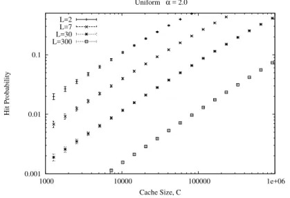
Figures 1 and 2 report the “hit” probability, as predicted by Che’s approximation, vs the cache size for different values of the exponentαand the content life span L, respectively. For each estimate, the figures show also the interval in which the exact
0.001 0.01 0.1 1000 10000 100000 1e+06 Hit Probability Cache Size, C Uniform L= 30 α=1.8 α=2.0 α=2.2 α=3.0
Fig. 1. phitversus cache size for different values of the exponentα >1and content life span
L= 30. 0.001 0.01 0.1 1000 10000 100000 1e+06 Hit Probability Cache Size, C Uniform α = 2.0 L=2 L=7 L=30 L=300
Fig. 2.phitversus cache size for different values of the content life spanLand exponentα= 2.
value of the “hit” probability falls as given by Proposition 3.14. All computations have been carried out while guaranteeing relative numerical errors smaller than 10−2. Some selected results are additionally reported in Table 1. Note that in all cases of practical relevance (i.e., for values of the “hit” probability exceeding 10−2) Che’s approximation leads to negligible errors. The surprisingly good degree of accuracy entailed by Che’s approximation, which has been already experimentally (i.e., against simulations) observed by several authors [15, 24], is now confirmed even for the SNM. Further numerical results providing useful insights on the cache performance can be found in [22].
Table 1
Numerical values for the Che approximation of the “hit” probability (phit,Che) and for the lower (phit) and the upper (phit) bounds of the true “hit” probability.
α L C phit,Che phit phit C phit,Che phit phit
1.8 30 10240 0.019596 0.018880 0.020313 163840 0.144328 0.143126 0.145529 2.0 2 10240 0.109252 0.105353 0.113151 163840 0.671657 0.669498 0.673815 2.0 7 10240 0.039790 0.038232 0.041348 163840 0.343061 0.340319 0.345802 2.0 30 10240 0.011657 0.011158 0.012156 163840 0.114597 0.113516 0.115677 2.0 300 10240 0.001555 0.001480 0.001629 163840 0.017497 0.017305 0.017688 2.2 30 10240 0.008125 0.007747 0.008504 163840 0.096641 0.095651 0.097630 3.0 30 10240 0.004524 0.004293 0.004755 163840 0.068667 0.067871 0.069464 REFERENCES
[1] G. Bianchi et al.,Check before storing: What is the performance price of content integrity verification in LRU caching?ACM Comput. Comm. Rev., 43 (2013), pp. 59–67. [2] L. Bondesson,Shot noise processes and shot noise distributions, In Encyclopedia of Statistical
Sciences, Wiley, New York, 1988, pp. 448–452.
[3] C. Bordenave and G. L. Torrisi, Monte Carlo methods for sensitivity analysis of Poisson driven stochastic systems, and applications. Adv. Appl. Probab., 40 (2008), pp. 293–320.
[4] H. Che, Y. Tung, and Z. Wang,Hierarchical Web caching systems: Modeling, design and experimental results. IEEE J. Selected Areas Commun., 20 (2002), pp. 1305–1314. [5] E. Coffman and P. Denning,Operating Systems Theory, Prentice-Hall, Englewood Cliffs,
NJ, 1974.
[6] R. Crane and D. Sornette, Robust dynamic classes revealed by measuring the response
function of a social system. Proc. Natl. Acad. Sci., 105 (2008), pp. 15649–15653. [7] D. J. Daley and D. Vere-Jones,An Introduction to the Theory of Point Processes, VolI,
Springer, New York, 2003.
[8] D. J. Daley and D. Vere-Jones,An Introduction to the Theory of Point Processes, Vol.II, Springer, New York, 2008.
[9] A. Dan and D. Towsley,An approximate analysis of the LRU and FIFO buffer replacement schemes. SIGMETRICS Perform. Eval. Rev., 18 (1990), pp. 143–152.
[10] A. Dembo and O. Zeitouni, Large Deviation Techniques and Applications, Springer, New York, 1998.
[11] P. M. Deshpande, K. Ramasamy, A. Shukla, and J. F. Naughton,Caching
multidimen-sional queries using chunks, in Proceedings of SIGMOD, 98, ACM, 1998.
[12] N. G. Duffield and W. Whitt,Large deviations of inverse processes with nonlinear scalings. Ann. Appl. Probab., 8 (1998), pp. 995–1026.
[13] K. Duffy and G. L. Torrisi,Sample path large deviations of Poisson shot noise with heavy tail semi-exponential distributions, J. Appl. Probab. 48 (2011), pp. 688–698.
[14] N. C. Fofack et al.,Performance evaluation of hierarchical TTL-based cache networks, Com-put. Networks, 65 (2014), pp. 212–231.
[15] C. Fricker, P. Robert, and J. Roberts,A versatile and accurate approximation for LRU cache performance, in Proceedings of ITC, Krakow, Poland, 2012, pp. 1–8.
[16] A. Ganesh, C. Macci, and G. L. Torrisi,Sample path large deviations principles for Poisson shot noise processes, and applications, Electron. J. Probab., 10 (2005), pp. 1026–1043. [17] A. Ganesh and G. L. Torrisi,A class of risk processes with delayed claims: Ruin probability
estimates under heavy tail conditions, J. Appl. Probab., 43 (2006), pp. 916–926.
[18] A. Ganesh, C. Macci, and G. L. Torrisi,A class of risk processes with reserve-dependent premium rate: Sample path large deviations and importance sampling, Queueing Syst., 55 (2007), pp. 83–94.
[19] V. Jacobson et al., Networking named content, in Proceedings of CoNEXT, Rome, Italy, ACM, 2009.
[20] W. Jiang et al.,Orchestrating massively distributed CDNs, in Proceedings of CoNEXT, Nice, France, ACM, 2012.
[21] K. Kylakoski and J. Virtamo,Cache replacement algorithms for the renewal arrival model, in Proceedings of the 14th Nordic Teletraffic Seminar, Copenhagen, Denmark, 1998, pp. 139–148.
[22] E. Leonardi and G. L. Torrisi,Least recently used caches under the shot noise model, in Proceedings of INFOCOM, Hong Kong, IEEE, 2015, pp. 2281–2289.
[23] S. B. Lowen and M. C. Teich,Power-law shot noise, IEEE Trans. Inform. Theory, 36 (1990), pp. 1302–1318.
[24] V. Martina et al.,A unified approach to the performance analysis of caching systems, in Proceedings of INFOCOM, Toronto, IEEE, 2014, pp. 2040–2048.
[25] J. Moller and G. L. Torrisi,Generalised shot noise Cox processes, Adv. Appl. Probab., 37
(2005), pp. 47–74.
[26] I. Nourdin and G. Peccati, Normal Approximation with Malliavin Calculus, Cambridge University Press, Cambridge, UK, 2012.
[27] G. Peccati, J. L. Sol´e, M. S. Taqqu, and F. Utzet,Stein’s method and normal approxima-tion of Poisson funcapproxima-tionals, Ann. Probab., 38 (2010), pp. 443–478.
[28] M. Penrose,Random Geometric Graphs, Oxford University Press, New York, 2004.
[29] I. Psaras, W. K. Chai, and G. Pavlou, Probabilistic methods in network caching for information-centric networks, presented at the ICN Workshop on Information-Centric Net-working, 2012.
[30] E. J. Rosensweig et al.,Approximate models for general cache networks, in Proceedings of INFOCOM, San Diego, IEEE, 2010, pp. 1–9.
[31] G. Stabile and G. L. Torrisi,Large deviations of Poisson shot noise processes, under heavy tail semi-exponential conditions, Statist. Probab. Lett., 80 (2010), pp. 1200–1209. [32] G. L. Torrisi,Simulating the ruin probability of risk processes with delay in claim settlement,
Stoch. Proc. Appl., 112 (2004), pp. 225–244.
[33] S. Traverso et al.,Temporal locality in today’s content caching: Why it matters and how to model it, ACM Comput. Comm. Rev., 43 (2013), pp. 5–12.
[34] S. Traverso et al.,Unravelling the impact of temporal and geographical locality in content caching systems, IEEE Trans. Multimedia, 17 (2015), pp. 1839–1854.