GAUSSIAN RADIAL GROWTH
K
RISTJANA´Y
RJ ´
ONSDOTTIR AND´
E
VAB
V
EDELJ
ENSENDepartment of Mathematical Sciences, University of Aarhus, Ny Munkegade, DK-8000, Aarhus C, Denmark e-mail: [email protected]
(Accepted May 4, 2005)
ABSTRACT
The growth of planar and spatial objects is often modelled using one-dimensional size parameters,e.g., volume, area or average width. We take a more detailed approach and model how the boundary of a growing object expands in time. We mainly consider star-shaped planar objects. The model can be regarded as a dynamic deformable template model. The limiting shape of the object may be circular but this is only one possibility among a range of limiting shapes. An application to tumour growth is presented. A 3D version of the model is presented and an extension of the model, involving time series, is briefly touched upon.
Keywords: Fourier expansion, Gaussian process, growth pattern, periodic stationary, radius vector function, shape, star-shaped objects, transformation.
INTRODUCTION
Modelling of biological growth patterns is a rapidly developing field of mathematical biology. Its state-of-the-art was explored at the successful conference On Growth and Form, held in 1998 in honour of D’Arcy Thompson (1860–1948) and his famous book, cf. Thompson (1917). Out of the conference grew a monograph which contains substantial biological material and an overview of mathematical modelling of spatio-temporal systems, cf. Chaplain et al. (1999). Examples of growth mechanisms studied are growth of capillary networks, skeletal growth and tumour growth.
Modelling of tumour growth has attracted particular interest in recent years. Tumour growth was one of the high priority topics of the recent multidisciplinary conference arranged by the European Society for Mathematical and Theoretical Biology in July 2002. More than 500 scientists from a wide range of disciplines participated. One of the subjects discussed was pattern formation problems, relating to tumour formation and progression, in particular the question of tumour shape.
The models suggested for tumour growth are either continuous or discrete. In Murray (2003), the continuous approach is explained in relation to brain tumours. The simplest models involve only total number of cells in the tumour, with growth of the tumour usually assumed to be exponential, Gompertzian or logistic (Swan, 1987; Marusicet al., 1994). More powerful deterministic models describe the change of the spatial arrangement of the cells under tumour growth. The discrete models are most often
cellular automaton models, cf. Qi et al. (1993) and Kansalet al.(2000).
The growth literature contains very few examples of statistical modelling and analysis of growth patterns. An exception is the paper by Cressie and Hulting (1992). Growth of a planar star-shaped object is here modelled, using a sequence of Boolean models. The objectYt+1 at timet+1 is the union of independent
random compact sets placed at uniform random positions inside the objectYt at timet. More formally,
Yt+1=∪{Z(xi):xi∈Yt},
where {xi} is a homogeneous Poisson point process
in the plane and Z(xi) is a random compact set
with position xi. Note that this model is Markov
since Yt+1 only depends on the previous objects via
Yt. The model is applied to describe the growth
pattern of human breast cancer cell islands. Practical methods of estimating the model parameters, using the information of the complete growth pattern, are devised. A related continuous model has recently been discussed in Deijfen (2003). The object Yt is
here a connected union of randomly sized Euclidean balls, emerging at exponentially distributed times. It is shown that the asymptotic shape is spherical.
In the present paper, we propose a Gaussian radial growth model for star-shaped planar objects. The model is a dynamic version of the p−order shape
model introduced in Hobolthet al.(2003). The object at timet+1 is a stochastic transformation of the object
at time t such that the radius vector function of the object fulfils
whereZt is a cyclic Gaussian process. The coefficients
of the Fourier series ofZt
Zt(θ) =µt+ ∞
∑
k=1
[At,kcos(kθ) +Bt,ksin(kθ)], (1)
θ ∈[0,2π), have important geometric interpretations
relating to the growth process. The overall growth from timettot+1 is determined by the parameterµt. The
coefficients At,1 andBt,1 determine the asymmetry of
growth from timet tot+1, while At,k andBt,k affect
how the growth appears globally for small k≥2 and
locally for large k≥2. Under the proposed p-order
growth model
At,k∼Bt,k∼N(0,λt,k), k=2,3, . . . ,
At,k, Bt,k, k = 2,3, . . ., independent, where the
variances satisfy the following regression model λ−1
t,k =αt+βt(k2p−22p), k=2,3, . . . .
The organization of the paper is as follows: in the first section, we introduce the Gaussian radial growth model. Then, we study the induced distributions of object size and shape under the radial growth model. After that, an application to tumour growth is discussed and a statistical analysis of a growth pattern is presented. An extension of the model, involving time series, is then briefly described. Finally, a 3D version of the model is presented.
THE GAUSSIAN RADIAL GROWTH
MODEL
Consider a planar bounded and topologically closed object with size and shape changing over time. The object at time t is denoted by Yt ⊂ R2, t =
0,1,2, . . .. We suppose that Yt is star-shaped with
respect to a pointz∈R2for allt. Then, the boundary
ofYt can be determined by its radius vector function
Rt={Rt(θ):θ∈[0,2π)}with respect toz, where
Rt(θ) =max{r:z+r(cosθ,sinθ)∈Yt},
θ ∈[0,2π). In Hobolth et al. (2003), a deformable
template model is introduced, describing a random planar object as a stochastic deformation of a known star-shaped template, see also the closely related models described in Hobolth and Jensen (2000), Kent et al. (2000) and Hobolth et al. (2002). We use this approach here and describe the object at timet+1 as
a stochastic transformation of the object at timet, such that
Rt+1(θ) =Rt(θ) +Zt(θ), θ∈[0,2π). (2)
Here,{Zt}is a series of independent stationary cyclic
Gaussian processes with Zt short for {Zt(θ) :θ ∈
[0,2π)}. The processZt is stationary if the distribution
ofZt(θ+θ0)−Zt(θ)does not depend onθ, while the
process is said to be cyclic if Zt(θ+2πk) = Zt(θ),
for allk∈Z. The initial valueR0of the radius vector
function is assumed to be known.
Note thatYt is used as a template in the stochastic
transformation, resulting in Yt+1. The increment
processZt can be written as
Zt(θ) =µt+Ut(θ), θ∈[0,2π),
where µt ∈Rrepresents a constant radial addition at
timetandUt a stochastic deformation with mean zero
of the expanded object with radius vector function Rt +µt, cf. Fig. 1. (The object with radius vector
functionRt+µt is in geometric tomography known as
the radial sum ofYt and a circular disc of radiusµt,cf.
Gardner (1995).)
Fig. 1.The object Yt+1 is a stochastic transformation
of the object Yt (grey), using a constant radial addition
(shown stippled) followed by a deformation.
Because of the independence of theZts, the model
is Markov in time, in the sense that it uses information about the object at the immediate past to describe the object at the present time. More specifically, under Eq. 2 the conditional distribution ofRt+1 given
Rt, . . . ,R0depends only onRt. The model suggested in
Cressie and Hulting (1992) possesses a similar Markov property.
If Yt is non-circular, it can be natural to extend
the model (Eq. 2), using an increasing time change function Γt :[0,2π]→ [0,1] such that Zt◦Γ−t 1 is a
stationary stochastic process on[0,1]. If the boundary
length ofYt is finite, one possibility is to choose
Γt(θ) = LLt(θ)
t(2π) , (3)
where Lt(θ) is the distance travelled along the
boundary ofYt between the points indexed by 0 and
ofYt is expected to be approximately circular, since
E(Zt(θ)) =µt does not depend onθ∈[0,2π).
The following result is important for the construction of parametric models in the framework of model (Eq. 2). The result also implies a simple simulation procedure for a stationary cyclic Gaussian process on[0,2π).
Proposition 2.1 The process Zt is a stationary cyclic
Gaussian process on[0,2π) with mean µt ∈R if and
only if there exist λt,k ≥0,k =0,1,2, . . ., such that ∑∞k=0λt,k<∞and
Zt(θ) =At,0+
∞
∑
k=1
[At,kcos(kθ) +Bt,ksin(kθ)],
θ ∈[0,2π), where At,0, At,k, Bt,k, k = 1,2, . . . , are
all independent, At,0 ∼N(µt,λt,0) and At,k ∼Bt,k ∼
N(0,λt,k).
The proof of Proposition 2.1 is not complicated. Given a stationary cyclic Gaussian processZt on[0,2π)with
meanµt, consider the stochastic Fourier expansion of
Zt. Then, simple calculations involving the stochastic
Fourier coefficients give the result. The other assertion is trivial.
Note that in Proposition 2.1, the λt,ks are allowed
to be zero, meaning thatAt,k≡0, almost surely.
The Fourier coefficients
At,0=21π Z 2π
0 Zt(θ)dθ,
At,k=π1 Z 2π
0 Zt(θ)cos(kθ)dθ , (4)
Bt,k=π1 Z 2π
0 Zt(θ)sin(θk)dθ, (5)
k=1,2, . . ., have interesting geometric interpretations relating to the growth process. It is clear that the coefficient At,0 determines the overall growth from
Yt to Yt+1. The Fourier coefficients At,1 and Bt,1
play also a special role. Numerically large values of the coefficients will imply an asymmetric growth from Yt to Yt+1. In order to interpret geometrically
the remaining Fourier coefficients At,k and Bt,k, k =
2,3, . . ., let us consider an increment process for which all Fourier coefficients except those of order 0 andk are zero,
Zt(θ) =At,0+At,kcos(kθ) +Bt,ksin(kθ),
θ∈[0,2π). Such a process exhibitsk-fold symmetry,
i.e.,
Zt
³
θ+2πi
k ´
, i=0,1, . . . ,k−1,
θ ∈[0,2π), does not depend oni. Therefore,At,k and
Bt,kaffect how the growth appears globally for smallk
and locally for large k. The variancesλt,k control the
magnitude of the spread of the Fourier coefficients. Since the zero- and first-order Fourier coefficients play a special role in relation to the growth process and may in applications well depend on explanatory variables, we shall desist from specific modelling of these coefficients. In the following we will assume that At,0 =µt is deterministic. Furthermore, we suppose
thatAt,1=Bt,1=0 or, equivalently, we concentrate on modelling
Zt(θ)−At,1cosθ−Bt,1sinθ, θ∈[0,2π).
A special case of the Gaussian radial growth model is the p-order growth model. This model is inspired by the p-order model described in Hobolth et al.(2003), where the stochastic deformation process is a stationary Gaussian process with an attractive covariance structure, described below. The model is called p-order because it can be derived as a limit of discrete p-order Markov models defined on a finite, systematic set of anglesθ,cf.Hobolthet al.(2002).
Definition 2.2 A stochastic processY ={Y(θ):θ ∈ [0,2π)} follows a p-order modelwith p> 12, if there existµ ∈R,α,β>0, such that
Y(θ) =µ+
∞
∑
k=2
[Akcos(kθ) +Bksin(kθ)],
θ ∈ [0,2π), where Ak ∼ Bk ∼ N(0,λk) are all
independent and λ−1
k =α+β(k2p−22p), k=2,3, . . . .
IfY follows a p−order model, we will writeY ∼
Gp(µ,α,β). Clearly,µis the mean ofY. Furthermore,
the covariance function ofY is of the form
σ(θ) =Cov(Y(0),Y(θ)) =
∞
∑
k=2
λkcos(kθ)
=
∞
∑
k=2
cos(kθ)
α+β(k2p−22p) ,
θ ∈[0,2π). The parameters α and β determine the variance of lower order and higher order Fourier coefficients, respectively. Furthermore, p determines the smoothness of the curveY. In fact, the curveY is k−1 times continuously differentiable wherek is the
unique integer satisfying p∈(k−12,k+12] (Hobolth
et al., 2003). Note that the first Fourier coefficients of Y are set to zero.
We can now give the definition of the p−order
Definition 2.3 The seriesZ={Zt}follows ap−order
growth model if the Zts are independent and Zt ∼
Gp(µt,αt,βt)for allt.
The parametersαt andβt determine, respectively,
the global and local appearance of growth from Yt
to Yt+1. As before, p determines the smoothness of
the curves Zt. The overall growth pattern is specified
by the µts. Their actual form depends on the specific
application. Tumour growth has often been described by a Gompertz growth pattern
κt =κ0exp hη
γ(1−exp(−γt))
i ,
whereκtis the average radius at timetandηandγare
positive parameters determining the growth, implying that
µt=κt
³ exphη
γ exp(−γt)(1−exp(−γ))
i −1´.
For more details, seee.g., Steel (1977).
Note that the p-order growth model allows for negative values ofRt(θ). However, the parametersµt,
αt andβt will be chosen such that this will practically
never occur.
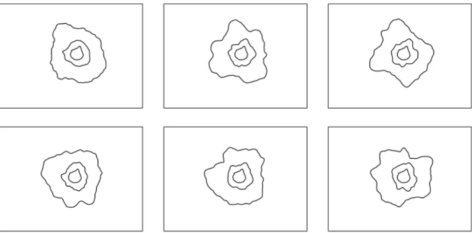
Fig. 2 shows simulations of the increment process Zt from timet tot+1 for different values of αt and
βt under the second-order growth model,i.e., p=2.
A large value of αt gives increments that are fairly
constant while a small value of αt provides a more
irregular growth on a global scale. The parameter βt
controls the local appearance of the increment process, the smaller βt the more pronounced irregularity on a
local scale.
Fig. 2. Simulated objects under the second-order growth model. The object at time t is fixed while the object at time t+1 is simulated under the indicated
values ofαt andβt.
DISTRIBUTIONAL RESULTS
In this section, we study the induced distribution of object size and shape under thep-order growth model. The limiting shape may be circular but, as we shall see, there is a whole range of possibilities.
Unless otherwise explicitly stated, we assume that R0≡0.We then have forθ∈[0,2π)
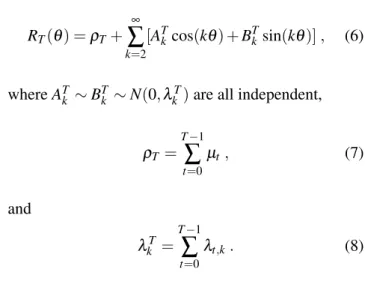
RT(θ) =ρT+ ∞
∑
k=2
[ATk cos(kθ) +BTk sin(kθ)], (6)
whereAT
k ∼BTk ∼N(0,λkT)are all independent,
ρT = T−1
∑
t=0
µt , (7)
and
λT k =
T−1
∑
t=0
λt,k. (8)
The shape of the object at time T will be represented by its normalized radius vector function
RT
E(RT(0)) =
RT
ρT,
which can be regarded as a continuous analogue of the standardized vertex transformation vector in shape theory,cf.Hobolthet al.(2002).
Under the assumption of independent increments, the distribution of the area of the object at time T, A(YT), is known, provided that the radius-vector
functionRT is positive.
Proposition 3.1 Assume that the radius vector function RT of the object YT is positive and that it
satisfies Eqs. 6–8. Then,
A(YT)∼πρT2+π ∞
∑
k=2
λT kVk,
where Vk, k = 2,3, . . ., are mutually independent
Proof.The area of the object at timeT is
A(YT) =12
Z 2π
0 RT(θ)
2dθ .
Note that since
∞
∑
k=2
(ATk)2+ (BTk)2<∞, almost surely,
we have that A(YT)<∞, almost surely. Using Eq. 6
and Parseval’s equation, we get that
A(YT) =πρT2+π2 ∞
∑
k=2
[(ATk)2+ (BTk)2]
=πρT2+π
∞
∑
k=2
λT k Vk,
where Vk, k = 2,3, . . ., are mutually independent
exponentially distributed random variables with
mean 1. ¤
The distribution of the area of YT is thus a sum of
independent Gamma distributed random variables. The saddlepoint approximation of such a distribution is easily derived,cf.Jensen (1992).
It does not seem possible to get a correspondingly simple result for the distribution of the boundary length ofYT. This seems apparent from the expression for the
boundary length ofYT
Z 2π
0 q
R0
T(θ)2+RT(θ)2dθ,
which is valid in the case whereRT is differentiable.
As we shall see now, the class of p-order growth models is quite rich in the sense that the shape of the limiting object, represented by its normalized radius vector function, may be distributed according to any p-order modelGp(1,α,β)with mean 1. For large values
ofα andβ, the shape is close to circular.
Let us consider the p-order growth model with proportional parameters, i.e., αt =γβt. Equivalently,
we assume that there exists a sequence{τt}of positive
real numbers such that
Zt =µt+τtXt (9)
and{Xt} are independent and identicallyGp(0,α,β)
distributed. If σ2 = Var(Xt(θ)), then Zt(θ) ∼
N(µt,τt2σ2)under Eq. 9.
Examples of choices ofτt areτt =1,√µt orρt+1,
cf.Eq. 7. Ifτt=1, the variance of the incrementZt(θ)
is constant in time. If τt =√µt, we obviously need
that µt ≥0 for all t and we have that Var(Zt(θ))∝
E(Zt(θ))such that the variance of the incrementZt(θ)
is proportional to the average increase in the radius at timet. Ifτt =ρt+1, then the distribution of the shape
of the object defined by the radius vector function
{ρt+Zt(θ): θ ∈[0,2π)}
is constant in time,i.e., the distribution of
ρt+Zt(θ)
E(ρt+Zt(θ))
does not depend ont.
In the proposition below, we show that under Eq. 9 the shape of Yt is distributed according to a p-order
model.
Proposition 3.2 Suppose that Z = {Zt} satisfies
Eq. 9 where Xt, t = 0,1,2, . . ., are independent
and identically Gp(0,α,β)−distributed. Then, the
normalized radius vector function ofYT is distributed
as
RT
E(RT(0))∼Gp(1,α¯T,β¯T)
where
¯
αT =αρT2/ T−1
∑
t=0
τ2
t, β¯T =βρT2/ T−1
∑
t=0
τ2
t .
Proof.It suffices to show that
Cov(RT(0),RT(θ))
[E(RT(0))]2 =
∞
∑
k=2
cos(kθ)
¯
αT+β¯T(k2p−22p) .
Using Eq. 6 and Eq. 9, we find
Cov(RT(0),RT(θ))
[E(RT(0)]2]
= 1
ρ2
T ∞
∑
k=2
λT
k cos(kθ)
= 1
ρ2
T ∞
∑
k=2
T−1
∑
t=0
τ2
t cos
(kθ)
α+β(k2p−22p)
=
∞
∑
k=2
cos(kθ)
¯
αT+β¯T(k2p−22p).
Example 3.3 (Constant increment growth) Let the situation be as in Proposition 3.2 with µt =µ and
τt=1 in Eq. 9. The increment processesZtare thereby
independent and identically distributed. It follows from Proposition 3.2 that
RT
ERT(0) ∼Gp(1,α¯T,
¯ βT),
where ¯αT =Tµ2α and ¯βT =Tµ2β. Since ¯αT → ∞
and ¯βT →∞ for T →∞, the boundary of the object
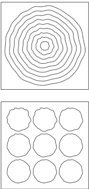
becomes more circular and smooth asT increases. An example is shown in Fig. 4. The limiting object has circular shape.
Example 3.4 (Wiener growth) Let the situation be as in Proposition 3.2 with µt arbitrary and τt =√µt
in Eq. 9. This special case is called a Wiener growth model since Var(RT) ∝E(RT). If µt = µ such that
ρT =Tµ, the process is called a Wiener process with
linear drift. If ρT = δTψ for some δ,ψ > 0, then
RT−ρT satisfies
Rat−ρat∼aH(Rt−ρt), a≥0, (10)
with parameterH=ψ2, which is a discrete analogue of self-similarity,cf.Sato (1999). Notice that
RT
ERT(0) ∼Gp(1,αρT,βρT).
If ρT → ρ < ∞, the limiting object can have any
stochastic shape determined byGp(1,αρ,βρ).
Example 3.5 Let the situation be as in Proposition 3.2 with µt arbitrary and τt = ρt+1 in Eq. 9. The
normalized radius vector function is distributed as RT
ERT(0) ∼Gp
µ
1,α ρ
2
T ∑tT=1ρt2
,β ρ
2
T ∑tT=1ρt2
¶ .
Ifρ2
T/∑Tt=1ρt2→0 asT→∞, the objects become more
irregular both globally and locally asT increases. An example is shown in Fig. 4.
AN APPLICATION
For illustrative purposes, we consider a data set consisting of human breast cancer cell islands, which have been observed in vitro in a nutrient medium on a flat dish. This data set has earlier been analysed in Cressie and Hulting (1992). Three profiles of cancer cell islands are available. The data set is presented in the upper left corner of Fig. 5.
Fig. 3. Top: Simulated growth pattern under the constant increment second-order growth model. Bottom: The corresponding normalized profiles, representing the shape of the object.
Fig. 5.The tumour growth data (upper left corner) and simulations under the second-order growth model with µt,αt andβt replaced by the maximum likelihood estimates.
The centre of mass ofY0is used as reference point.
The data consist of increments
zt
³2πi nt
´
, i=0,1, . . . ,nt−1,
in nt directions, equidistant in angle, t = 0,1. For
convenience,zt is normalized with the average radius
ofY0. Only digitized images are available. As nt, we
have used approximately 25% of the number of pixels on the boundary of the digitized image ofYt,t=0,1.
Under the p-order growth model, the mean value parameters µt can be estimated by the average
observed increment at timet. The variance parameters can be estimated using the likelihood function
L(α0,β0,α1,β1) =
∏
t=0,1
Lt(αt,βt),
whereLt(αt,βt)is the likelihood function based on the
Fourier coefficientsAt,k andBt,k ofZt of orderk≤Kt,
say. SinceAt,k ∼Bt,k ∼N(0,λt,k) are all independent and
λ−1
t,k =αt+βt(k2p−22p), k=2,3, . . . ,
the likelihood becomes
Lt(αt,βt) = Kt
∏
k=2
[αt+βt(k2p−22p)]
×exp(−ct,k[αt+βt(k2p−22p)]), (11)
where ct,k = [at2,k+b2t,k]/2 are the observed phase
amplitudes. In applications,at,k and bt,k are replaced
by discrete versions of the integrals in Eq. 4.
The choice of the cut-off value Kt is very
important. Clearly, Kt must not be too large in order
to avoid that the estimates are influenced by the digitization effects. On the other hand, if the cut-off value Kt is too small information about the
growth pattern is lost. The choice of Kt should be
an intermediate value for which the estimate of the local parameterβt is stable. Whether a specific choice
of Kt is appropriate can also be judged from visual
inspection of simulated growth patterns under the estimated model.
For the two increments z0 and z1, we used (n0,K0) = (60,25) and (n1,K1) = (120,30),
respectively. The maximum likelihood estimates under the second-order growth model are
ˆ
µ0=1.04,log(αˆ0) =5.29,log(βˆ0) =−1.88,
ˆ
µ1=2.53,log(αˆ1) =3.18,log(βˆ1) =−3.54.
The estimated regression curves
ˆ
λt,k= 1
ˆ
αt+βˆt(k4−24)
, t=0,1 k=2,3, . . .
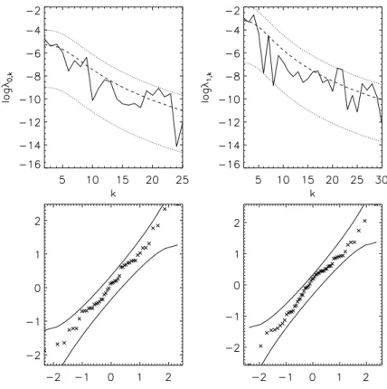
are shown in Fig. 6, together with 95% confidence limits for the logarithm of the phase amplitudes. The model fits the data well which can also be seen from the fractile diagrams (QQ plots) for the normalized Fourier coefficients, also shown in Fig. 6.
Simulations under the second-order growth model withµt,αt andβtreplaced by the maximum likelihood
estimates are shown in Fig. 5.
Since the data set only contains two increments, it is not meaningful to try to evaluate the Markov assumption. Note also that the Zts are assumed
independent but not necessarily identically distributed. If
Fig. 6.The two upper figures show the observed phase amplitudes (full-drawn lines) together with the estimated regression curves (stippled) and 95%confidence limits, t=0,1. The two lower figures show fractile diagrams (QQ plots) for the normalized Fourier coefficients at,k/
q ˆ
λt,k, bt,k/
q ˆ
λt,k together with 95%confidence limits,
t=0,1.
we have that p
βt(Zt−µt)∼Gp(0,γ,1)
are independent and identically distributed. Thus, under the assumption (Eq. 12) of proportionality and with sufficient number T of time points, we can examine the independence of
p
βt(Zt(θ)−µt), t=0,1, . . . ,T−1,
for selected values ofθ∈[0,2π), using a runs test, for instance.
A TIME SERIES EXTENSION
Let us suppose thatZt =µt+τtXt,
where X = {Xt} is a stationary time series of
cyclic Gaussian processes satisfying the ARMA model equation
Xt−φ1Xt−1− ··· −φrXt−r
=Wt−ψ1Wt−1− ··· −ψsWt−s. (13)
We assume that W ={Wt} is a sequence of i.i.d.
stationary cyclic Gaussian processes on[0,2π)with
Wt ∼Gp(0,α,β).
If φi =0, i=1, . . . ,r, and ψj = 0, j =1, . . . ,s, Z
follows the p-order growth model with independent increments, treated in the previous sections.
Under the general ARMA model (Eq. 13), the Fourier coefficients ofXandWof a given order follow a one-dimensional ARMA model. Furthermore, for fixed θ ∈[0,2π), Xt(θ) follows a one-dimensional
ARMA model. Aspects of this time series approach has earlier been discussed in Alt (1999). An early example concerning year ring widths is discussed in Kronborg (1981).
Note that in the special case of a MA model (φ1= ···=φr=0), the marginal distribution ofZt belongs
to the class ofp-order models
where
αt =τ2 α
t[1+ψ12+···+ψs2]
,
βt =τ2 β
t[1+ψ12+···+ψs2]
.
Note also that in this caseZt andZt0are independent if
|t−t0|>s.
EXTENSION TO THREE
DIMENSIONS
The p-order growth model for planar objects can easily be extended to three dimensions. Consider a spatial bounded and topologically closed objectYt ⊂
R3which is star-shaped for alltwith respect toz∈R3.
Clearly the boundary of the object can be determined by
{z+Rt(θ,ϕ): θ∈[0,2π), ϕ∈[0,π]}, whereRt(θ,ϕ)is the distance fromzto the boundary
ofYt in direction
ω(θ,ϕ) = (sinϕcosθ,sinϕsinθ,cosϕ). In the same way as in the planar case we let the object Yt+1 be a stochastic transformation of the object Yt,
such that
Rt+1(θ,ϕ) =Rt(θ,ϕ) +Zt(θ,ϕ),
θ ∈ [0,2π), ϕ ∈[0,π], where {Zt} is a time series
of Gaussian procesess on[0,2π)×[0,π]. Writing the
stochastic processZt in terms of its Fourier-Legendre
series expansion we get,cf.Hobolth (2003),
Zt(θ,ϕ) = ∞
∑
n=0
m=n
∑
m=−nAt,n,mφn,m
(θ,ϕ),
whereφn,m are the spherical harmonics andAt,n,m are
random coefficients. Using a similar reasoning as in Hobolth (2003) it can be seen thatAt,0,0determines the
overall growth fromYt toYt+1. The coefficientsAt,1,m,
m=−1,0,1, control the asymmetry of growth, and the remaining coefficientsAt,n,mforn≥2,m=−n, . . . ,n,
affect how the growth appears globally for small n and locally for largen. A p-order growth model can be defined by assuming thatAt,0,0=µt,At,1,m=0 for
m=−1,0,1 and
At,n,m∼N(0,λt,n),
n=2,3, . . .,m=−n, . . . ,n, independent, where λ−1
t,n =αt+βt(n2p−22p).
As in the planar case, the increment processes may be chosen to be normal after a transformation. A simulation from such a model, where {Zt}is a series
of log-Gaussian processes, is shown in Fig. 6.
Fig. 7. Simulation from a 3D log-Gaussian radial growth model.
DISCUSSION
The p−order growth model has mainly been
suggested as a general tool for analyzing observed radial growth patterns. The model may, however, also be of interest as a building block in other modelling situations, for instance in models for tessellations where cells are created by radial growth from each point of a point process.
The p−order growth model can be extended
in various ways. It is obviously easy to modify the model such that the increments are Gaussian after a transformation. An example is log-Gaussian increments. If the number of increments observed is not too small it is also of interest to try to model the dependency in the seriesZ={Zt}. We have discussed
a time series approach. Another alternative is to look at L´evy based models,
Zt(θ) =
Z
At(θ)ht(a;θ)Z(da),
At(θ)∈B, whereB is the Borel field of[0,2π)×R
andZ is a L´evy basis on[0,2π)×R. A detailed study
of the L´evy based growth models is ongoing research in our group, cf. Schmiegel et al. (in preparation). These models can also be formulated in continuous time.
The likelihood used in the application is correct if the increments are independent. If the marginal distributions of the Zts belong to the class of p-order
models but theZts are dependent, the likelihood may
still be used as a pseudo-likelihood.
ACKNOWLEDGEMENTS
Dr. G.C. Buehring, University of California, Berkeley, is the source of the tumour growth data in Fig. 5. Sławomir Ra˙zniewski is thanked for designing the 3D simulation program used in Fig. 6. This work was supported in part by MaPhySto – Network in Mathematical Physics and Stochastics, funded by The Danish National Research Foundation and a grant from the Danish Natural Science Research Council.
REFERENCES
Alt W (1999). Statistics and dynamics of cellular shape changes. In: Chaplain MAJ, Singh GD, McLachlan JC, eds., On Growth and Form: Spatio-temporal Pattern Formation in Biology. Chichester: Wiley, 287–307. Chaplain MAJ, Singh GD, McLachlan JC (1999). On
Growth and Form: Spatio-temporal Pattern Formation in Biology. Chichester: Wiley.
Cressie N, Hulting FL (1992). A spatial statistical analysis of tumor growth. J Amer Statist Assoc 87:272–83. Deijfen M (2003). Asymptotic shape in a continuum growth
model. Adv Appl Probab SGSA 35:303–18.
Gardner R (1995). Geometric Tomography. New York: Cambridge University Press.
Hobolth A (2003). The spherical deformation model. Biostatistics 4:583–95.
Hobolth A, Jensen E (2000). Modelling stochastic changes in curve shape, with an application to cancer diagnostics. Adv Appl Probab SGSA 32:344–62. Hobolth A, Kent J, Dryden I (2002). On the relation between
edge and vertex modelling in shape analysis. Scand J Stat 29:355–74.
Hobolth A, Pedersen J, Jensen EBV (2003). A continuous
parametric shape model. Ann Inst Statist Math 55:227– 42.
Jensen J (1992). A note on a conjecture of H.E. Daniels. Rev Bras Probab Estat 6:85–95.
Kansal AR, Torquato S, Harsh GR, Chiocca EA, Deisboeck TS (2000). Simulated brain tumor growth dynamics using a three-dimensional cellular automaton. J Theor Biol 203:367–82.
Kent J, Dryden I, Anderson C (2000). Using circulant symmetry to model featureless objects. Biometrika 87:527–44.
Kronborg D (1981). Distribution of crosscorrelations in two-dimensional time series, with application to dendrochronology. Research report no. 72, Department of Theoretical Statistics, Institute of Mathematics, University of Aarhus.
Marusic M, Bajzer Z, Freyer JP, Vuk-Pavlovic S (1994). Analysis of growth of multicellular tumour spheroids by mathematical models. Cell Prolif 27:73–94.
Murray JD (2003). Mathematical Biology. II: Spatial Models and Biomedical Applications. Berlin: Springer-Verlag.
Qi AS, Zheng X, Du CY, Bao-Sheng A (1993). A cellular automaton model of cancerous growth. J Theor Biol 161:1–12.
Sato K (1999). L´evy Processes and Infinitely Divisable Distributions. Cambridge: Cambridge University Press. Steel GG (1977). Growth kinetics of tumours. Oxford:
Clarendon Press.
Swan GW (1987). Tumour growth models and cancer therapy. In: Thompson JR, Brown BR, eds., Cancer Modeling. New York: Marcel Dekker, 91–104.