Loughborough University
Institutional Repository
System failure modelling
using binary decision
diagrams
This item was submitted to Loughborough University's Institutional Repository by the/an author.
Additional Information:
• A Doctoral Thesis. Submitted in partial fullment of the requirements for
the award of Doctor of Philosophy of Loughborough University. Metadata Record: https://dspace.lboro.ac.uk/2134/12233
Publisher: cRasa Remenyte-Prescott
This item was submitted to Loughborough University as a PhD thesis by the author and is made available in the Institutional Repository
(https://dspace.lboro.ac.uk/) under the following Creative Commons Licence
conditions.
For the full text of this licence, please go to: http://creativecommons.org/licenses/by-nc-nd/2.5/
- - -
-University Library
I •
Lo1;1ghb.orough• Umvers1ty
Author/Filmg T1tle ....
f\.~.~E.r;(.Y.I~.:- f,f:?_f~!.~C::.JT
... ... ....
.
.... .. ... ....
.
....
.
... .
T
Class Mark
..
... ... ....
...
.... ...
... ... ...
.
... .
Please note that fines are charged on ALL
overdue items.
r
SYSTEM FAILURE MODELLING
USING BINARY DECISION DIAGRAMS
By
Rasa Remenyte-Prescott
A Doctoral Thests
submitted in parttal fulfilment of the requirements for the award of
Doctor of Philosophy of Loughborough Umversity
June, 2007
~-1
-
' lA llnn pr•-l ~. ~~'\1 ,..
,
"'~')l J P• 1...'" ~1,1; ; ,.,rv ---. DaterVC!V
r o'Z--
-·
--Cl as;-r
- ---Ace No C;;l-f;d3b
olr-'3 '0
"1
Abstract
The aim of th1s thesis is to develop the Binary DeciSIOn Diagram method for the analysis of coherent and non-coherent fault trees. At present the weii-known ite techmque for converting fault trees to BDDs IS used Difficulties appear when the ordering scheme for bas1c events needs to be chosen, because 1t can have a crucial effect on the size of a BDD An alternative method for constructmg BDDs from fault trees wh1ch addresses these difficulties has been proposed
The Binary DecisiOn Dmgram method provides an accurate and efficient tool for analysing coherent and non-coherent fault trees. The method IS used for the qual-itative and quantqual-itative analyses and it is a lot faster and more efficient than the conventional techniques of Fault Tree Analysis The Simplification techmques of fault trees prior to the BDD conversion have been applied and the method for the qualitative analysis of BDDs for coherent and non-coherent fault trees has been developed
A new method for the qualitative analysis of non-coherent fault trees has been proposed An analysis of the efficiency has been carried out, comparing the pro-posed method with the other existmg methods for calculating pnme implicant sets.
The main advantages and di~advantages of the methods have been identified.
The combined method of fault tree Simplification and the BDD approach has been applied to Phased Misswns This application contains coherent and non-coherent fault trees Methods to perform thmr simplification, converswn to BDDs, minimal cut sets/prime implicant sets calculatiOn, and the m1sswn unreliab1lity evaluation have been produced
r
Acknowledgments
First of all, I would hke to thank my supervisor Professor John Andrews for giv-ing me the chance to conduct this research, for h1s guidance and for always begiv-ing fnendly and helpful.
I am grateful to my fam1ly and friends here and back at home for their support and encouragement throughout this research.
I also would like to thank the people m the Risk and Reliability research group for the possib1hty to share ideas and keepmg up my motivation.
Fmally, thanks to Darren, my husband and colleague, for the endless insp1ratwn, continuous understandmg and invaluable fnendship.
-Contents
1 Introduction
1 1 Risk and Reliability Assessment
1.2 Fault Tree Analysis . 1.3 Binary Decision Dmgrams
1.4 Research Objectives .
2 Fault Tree Analysis
2.1 Introduction ..
2.2 Construction of Fault Tree 2 3 Quahtat1ve Analys1s . . .
2.3.1 Boolean Laws of Algebra
2.3.2 Example - Obtammg the Mmimal Cut Sets . 2 4 Quantitative Analysis
2.4 1 Structure Functwns . 2.4 2 Shannon's Theorem
2 4 3 General Method for the Calculation of the Top Event
Prob-1 1 2 3 4 5 5 5 7 9 10 11 12 13 ability . . . 14
2 4 3 1 Upper and lower bounds for system unavmlability 15
2 4 3 2 Minimal cut set upper bound 15
2.4 4 Top Event Frequency . .
2.4 4 1 Approximation for the system unconditional failure
intensity . . . .
2 4 4 2 Expected number of system failures .
2 4 5 Importance Measures . . 2 4 5.1 DetermmiStiC measures . 16 17 17 17 18
2 4 5.2 Probabilistic measures of system unavailability 18
2 5 SimplificatiOn of the Fault Tree Structure . . . 19
2 5 1 1 Introduction . . . 20
2 5.1 1.1 Reduction techmque 20
2 5 1 2 Worked example of the reduction technique 21
2.5 1 2 1 Contraction 22
2.5 1 2 2 Factorisation 2 5 1 2 3 Extraction 2 5.1 2.4 Absorption 2.5 1 3 Reduced fault tree
2.5.2 Fault Tree Modularisatwn
2 52 1 2 6 Summary .
Rauzy's algorithm
3 Binary Decision Diagrams 3 1 Introduction .
3.2 Properties of the BDD
3.2.1 Formation of the BDD Usmg If-Then-Else
3.3 Reductwn . . . 3 4 Modularisation 22 24 24 26 28 28 31 32 32 32 34 37 37 3.5 Qualitative Analysis 39
3 5.1 Incorporatmg Complex Events and Modules mto the Analysis 42
3 6 Quantitative Analysis . . 44
3 6.1 System Unavailability 44
3.6 2 System UnconditiOnal Failure Intensity 45
3 6 3 Worked Example 47
3.6 4 Incorporating Complex Events and Modules into the Analysis 48 3 6.4.1 Overview of the calculatwn procedure . . . 49
3.6.4 2 Unavailability of complex and modular events . . 50
3.6 4 3 Cnticahty of basic events withm complex events 50
3 6 4 4 Criticahty of basic events withm modules 53
3 6 5 The Algorithm for Incorporating Complex Events and Mod-ules into the Analysis .
3. 7 Summary . .
4 Component Connection Method for Building BDDs 4.1 Introduction 4 2 Connection Process 4 3 Rules of Simplification 54 55 56 56 56 62
4.4 Properties of the BDD Usmg the Component Connection Method 65 4 5 Measures of Efficiency
4.6 Selection Schemes m the Component ConnectiOn Method 4 6 1 Order of Basic Events SelectiOn
4.6 1.1 Order as hsted process
4 6 1 2 Defined ordenng
4 6 1 2.1 Neighbourhood ordermg schemes
4.6 1 2.2 Weighted ordering schemes . . .
66 68 68 68 69 70 74
4 6 2 Order of Inputs Selection for the Top-Down Technique 81
4.6.2.1 Order as hsted process . . . . 81
4 6 2 2 Ordering event mputs before gate inputs 81
4.6 2.3 Ordermg gate inputs accordmg to the number of
the1r event inputs . . . 81
4.6 3 Order of BDDs SelectiOn for the Bottom-Up Techmque 84
4.6 3.1 Order as hsted process . . . 84
4.6 3 2 According to a defined ordering of basic events 85
4.6 3 3 According to the number of available branches 87
4.6.4 Results . . . .. 4 6 4 1 Top-down technique 4 6.4.11 Summary results 88 90 90 4 6.4.1 2 Variable ordermg for the top-down approach 90
4 6 4 2 Bottom-up technique . . . 92
4 6 4.2 1 Summary results 92
4 6.4.2 2 Vanable ordering for the bottom-up
ap-proach. . 92
4 6 4 3 Comparison of top-down and bottom-up techmque 93
4.6.4 4 Bottom-up technique, chosen tnals 95
4.6.4 4 1 IntroductiOn 95
4.6.4.4 2 First tnal . . 96
4.6 4 4 3 Second trial . 97
4 6 4 4 4 Third tnal 98
4.6 4 4 5 Companson of the bottom-up techniques 100
4 7 Comparison Between the Component Connection and the ite method101
4 8 Sub-node Sharing . . . 104
4 8 1 Presentation of the Sub-node Sharing in Component
4 8 2 Comparison Between the ite and the Component Connection
Method Usmg the Sub-node Sharing 107
4 9 Hybrid method . . . 110
4.9.1 Presentation of the Method 111
4 9.2 Companson Between the ite and the Hybrid Method 116
4 9 2.1 Comparison between the Basic Hybnd method and
4 9.2 2
4 10 Summary . .
the ite technique . . . .
Companson between the Basic Hybrid Method and the Advanced Hybrid method
5 Non-coherent Systems 5.1 Introduction . . . .
5.2 Fault Tree Analysis of Non-coherent Fault Trees
5 2 1 Introduction
5.2.2 The Use of NOT Logic 5 2 3 Qualitative Analysis .
5 2 3 1 Calculation of prime 1mplicants
5 2 4 Quantitative Analys1s
5 2 4.1 Calculating the system unavailability .
117 119 122 124 124 124 124 125 128 128 130 130
5.2 4.2 Calculatmg the unconditional fa1lure intensity 131
5 2 4.3 Importance measures . . . . 132
5 3 Simplification Process of Non-coherent Fault Trees .
53 1 Faunet Reductwn in the Non-coherent Fault Tree Case
53 2 Lmear Modularisatwn m the Non-coherent FT Case 5.4 Summary .
134 134 138 139
6 The BDD Method for the Analysis of Non-coherent Fault Trees 140
6 1 Introduction . . . 140
6 2 Computmg the SFBDD m Non-coherent Case 6 3 Qualitative Analys1s . . . .
6 3 1 Coherent Approx1matwn
6 3 2 Ternary DeciSIOn Diagram Method
6 3 2.1 Computmg the TDD .
6 3 2 2 Mmimismg the TDD .
6 3 3 Established methods . .
6 3 3 1 Rauzy and Dutuit Meta-products BDD
141 142 143 143 145 148 151 151
6 3 3 1 1 MPPI algorithm
6 3.3.2 Zero-suppressed BDD Method .
6.3 3 2 1 Presentation of a ZBDD 6 3 3.2 2 DecompositiOn rule 6 3 3 2 3 Worked example
6.3 3 3 Labelled Vanable Method
152 156 156 157 158 160 6 3 3 3.1 Classification of variables 160 6 3 3.3.2 ConstructiOn of the 1-BDD 161 6 3.3.3.3 DeterminatiOn of prime implicants 163
6.3 3.3 4 Simplification of 1-BDD 164
6 3.4 Comparison of the Four Methods . . 6 3.4.1 TDD method results . . .
166 168
6 3 4 11 Vanable ordenng for the TDD method . 169
6.3.4.2 Meta-products method results . . . 170
6 3 4 2 1 Vanable ordermg for the MPPI method 171
6.3 4 3 ZBDD method results . . . 172
6 3.4.3.1 Variable ordering for the ZBDD method . 173
6.3.4 4 1-BDD method results . . . 174
6 3 4.4 1 Variable ordering for the 1-BDD method 175 6.3 5 Overall Vanable Ordering for the Qualitative Analys1s of
Non-coherent Fault Trees 6.4 Quantitative Analysis . 6.4.1 Introduction . . 6 4 2 System Unavailability 6 4 3 Importance Measures . 176 180 180 180 181
6.4.3 1 Birnbaum's measure of failure and repair importance181
6 4 3.1.1 The SFBDD method .
6 4.3 1.2 The 1-BDD method
6 4.3 1.3 The TDD method .
6 5 Hybrid Method in the Non-coherent Fault Tree Case 6 6 Summary . 182 183 185 187 189
7 Application of Proposed Methods in Phased Mission Analysis 193
7.1 Introduction . . . 193
7.2 Fault Tree Method for Phased M1ssion Analysis 194
7 4 Binary Decision Diagram Analysis for Phased Misswns 7.5 Summary . . . .
8 Computer Implementation of BDD Method
8 1 Introduction . 8 2 Overview .
8 3 Established Modules 8 3.1 Data Input Module
8 3.2 SimplificatiOn Module
8 3 3 BDD Conversion Module .
8.3 4 Quantitative Analysis Module
8 3.5 Qualitative Analys1s Module .
204 207 208 208 208 209 209 211 212 214 215 8 3 5.1 Minim1satwn module . 215
8 3 5 2 Calculation of mimmal cut sets 217
8 3 6 Component Connection Method . 219
8.3 7 Hybnd Method . . 223
8 3.8 Non-coherent FT Input Format and Conversion to SFBDD 224 8 3 9 Non-coherent Fault Tree Conversion to BDDs for the
Quali-tative Analys1s
9 Conclusions and Future Work
9 1 Summary of Work . . . . ..
9.11 Qualitative Analysis of Coherent Systems .
225 228 228 228
9 1 2 Component Connection Method 229
9 1 3 Qualitative Analysis of Non-coherent Systems 232
9 1 4 Applicatwn of Proposed Methods m Phased Misswn Analysis 235
9 2 Conclusions . 235
9.3 Future Work . 236
9.3.1 Component Connectwn Method 236
9 3 2 Applicatwn of Proposed Methods m Phased Misswn Analys1s 237
Nomenclature
A(t)
c
F(t) G,(q(t)) G;'(q(t)) G~(q(t)) K, n N Availability function Consequence of an event System unreliab1lity functionCrit1cality function for event z (Birnbaum's measure of importance) Component z failure cntJcality
Component z repair criticality Measure of importance for event z
Measure of failure importance for component or cut set z Measure of repair importance for component or cut set z Minimal cut set z
Number of components in a system
Number of mimmal cut sets (or pnme 1mplicant sets) Number of basic events in a prime 1mplicant set
Meta-products structure encoding prime 1mplicant sets for wh1ch x is irrelevant
P1 - Meta-products structure encoding prime 1mplicant sets
for which x IS failure relevant
PO - Meta-products structure encoding pnme implicant sets for wh1ch x 1s repair relevant
p
P(K,)
P[F]
Px,
Probability
Probability of existence of minimal cut set z Probability value of node Fin a BDD
Probability of bas1c events encoded in the path from the root vertex to the current node encodmg x,
po!,(q(t)) - Probab1lity of the path section from the 1 branch of a node encoding x, to a terminal vertex 1 in the BDD
po~. (q(t)) - Probability of the path sectwn from the 0 branch of a node encoding x, to a terminal vertex 1 m the BDD
po;;;c(q(t)) - Probability of the path sectiOn from the 1 branch of a node encoding x, to a termmal vertex 1 in the BDD via only 1 or 0 branches
of non-terminal nodes (excluding the probability of x,)
po~;c(q(t)) - Probability of the path section from the 0 branch of a node encodmg x,
to a termmal vertex 1 m the BDD via only 1 or 0 branches
of non-terminal nodes ( excludmg the probability of x,)
po~.(q(t)) - Probability of the path section from the 'C' branch of a node encoding x, to a terminal vertex 1 m the BD D via only 1 or 0 branches
of non-terminal nodes (excluding the probability of x,) prx,(q(t)) - Probability of the path section
Q(t) q,(t) R R(t) W(to, ti) Wsys(t) w,(t) wx,(t) v,(t) x, Z(q(t))
from the root vertex to the node encodmg x, in the BDD System unavailability (failure probability)
Component unavailability (failure probability)
Probability of a literal contained m any of the prime 1mplicant sets Rtsk
Reliability function
Failure relevance or Irrelevance of component z
Repair relevance or irrelevance of corn ponent z
Irrelevance of component z
Expected number of failures durmg the interval (
t
0 , t1)System unconditiOnal fatlure mtenstty Component unconditional failure mtensity
Unconditional failure intensity of mmimal cut set z
Unconditional repair mtensity of component z
Complex event
Binary indicator vanable for component states Probability of paths from the root vertex
>..(t) Conditwnal failure rate <f;(x) Structure function
1/J;
Fmlure criticahty function1/J~ Repair criticality functwn
p,(x) Binary mdicator functiOn for each mimmal cut set
Chapter 1
Introduction
1.1 Risk and Reliability Assessment
Reliability engmeering is a rapidly developmg field and is becoming mcreasingly important in various industnes and technologies It provides those theoretical and practical tools wh1ch can specify, design and predict the probability and capabil-Ity of components and systems to perform their required functwns for the desired period w1thout failure.
Reliability assessment techniques enable the calculation of the probability or fre-quency of system failure to be performed There are several measures that can be used to quantify system failure, mcluding system reliab1lity, availability and fa1lure intensity.
The relzabzlzty of a system, R(t), IS defined as the probab1lity that the system operates w1thout fa1lure for a spec1fied period of time under stated conditwns The unrelzabzlzty of a system, F(t), IS defined as the probability that the system has failed at least once in the mterval [0, t) g1ven that it was working at t
=
0 Smce both functwns are probabilistic.R(t)
+
F(t) = 1. (1 1)The system avazlabzlzty, A(t), is defined as the fractwn of total time that the system is able to perform Its required function. The unavazlabzlzty, Q(t), is defined as the fraction of total time that the system has fmled and is unable to perform its task Again, the relatiOnship between the two functions IS defined as:
The uncondztzonal Jazlure zntenszty, w(t), IS the rate that a system fails per umt
time at time
t
gtven that it was workmg at timet = 0. The rate that a system fails per unit ttme at ttme t given that tt was working at ttme t and at time t=
0 is defined as the condztzonal fazlure rate, >.(t). The dtfference between w(t) and >.(t)is that w(t) is based on the whole populatwn, whereas >.(t) considers only those components that are working at ttme t.
For major hazard assessments risk ts generally defined as the product of the con-sequences of a particular incident, C, and the probabthty over a time penod or frequency of tts occurrence, P
R=C·P (1.3)
The risk can be reduced by mimmising the consequences of the mctdent (C) or by reducing the probability or frequency of its occurrence (P) Rehabtlity assessment techmques evaluatmg the frequencies of incidents have been developed and the most widely used is Fault Tree Analysis, whtch is considered later in this chapter
After risks are tdentified and evaluated 1t must be judged tf they are 'accept-able' or whether the risk is too high and some modifications to the design of the system should be made m order to improve the system rehabthty. Although nsks can be decreased by spendmg money 1t is not posstble to avoid them enttrely. The dtfficulty faced by safety assessors is to convince regulators that the safety of a system ts at an acceptable level
1.2 Fault Tree Analysis
Fault Tree Analysts was developed by H A.Watson in the early 1960's. This is a deductive procedure for determmmg the causes of a particular system failure mode and the probability and frequency wtth which tt could occur. The fault tree dtagram represents the combmations of component fatlures and human errors that could combme to cause system failure. 'Top event' describes the system failure mode and branches below this event describe its causes. The events are redefined m terms of their causes, until each branch ends with a basic event
Kinetic Tree Theory, the technique for performing the quantttative analysis of fault trees, was presented in the early 1970's by Vesely [1]. Various system
rehabil-ity parameters, such as probabilrehabil-ity of top event ex1stence, frequency of top event occurrence and component importance measures can be calculated They are used to determme whether the risk of system fa1lure JS sufficiently small and therefore
whether or not the system meets the required safety standards
For large fault trees the analys1s can become computatwnally intensive and can reqmre the use of approximatwns Th1s IS the disadvantage of the conventional
method wh1ch leads to maccuracies in the calculations Th1s issue has led to the de-velopment of a new method for analysing fault trees, known as the Binary Decision D1agram techmque
1.3 Binary Decision Diagrams
The Bmary Decision Diagram (BDD) technique for Fault Tree Analysis was pre-sented by Rauzy [2]. This method converts a fault tree to a BDD, wh1ch encodes the log1c function of the fault tree. Conventwnal FTA techniques can be computa-twnally mtens1ve and sometimes inaccurate. The BDD method is an accurate and efficwnt method for system rehabihty assessment. F1rstly, the BDD method pro-vides an accurate quantification process because no approximations are required. Secondly the mmimal cut sets are not reqmred for the quantification process, there-fore, it makes the BDD method efficient The quahtat1ve analysis can be performed and minimal cut sets obtained if reqmred.
The s1ze of the BDD depends upon the order m wh1ch the bas1c events are con-sidered during the construction process A problem can occur 1f the choice of the ordermg scheme results in a t1me-consuming constructiOn process and a large BDD. No one ordering scheme w1ll produce the smallest poss1ble BDD from every fault tree
When NOT logic IS mcluded m the fault tree structure 1t becomes non-coherent
and 1ts analysis usmg the conventional techniques to produce prime implicant sets becomes even more problematic. BDDs offer advantages over the conventwnal methods for th1s class of fault trees. However, alternative techmques for convert-ing fault trees to BDDs can improve the efficiency of the approach still further
1.4 Research Objectives
The aim of this research is to improve the techmques which produce BDDs from fault trees and conduct the analysis. Four aspects are taken into consideratwn
In the previous research fault trees were reduced (applymg reduction and mod-ulansation) pnor to BDD conversiOn This can be used m fault tree quantifica-tion. The qualitative analysis usmg BDDs is extended to investigate the use of these reduced trees The goal of this aspect is to perform the full BDD analys1s and to obtain m1mmal cut sets m terms of basic events from the reduced fault trees
The second aspect explores a new fault tree to BDD conversion technique, as an alternative method to the well-known ite technique. The new method is based on connectmg previously generated BDD sectwns Th1s technique is presented for the analys1s of coherent fault trees D1fferent efficiency measures are used to mves-tJgate the optimum connection technique.
The th1rd aspect proposes a new method for converting non-coherent fault trees to BDDs The new approach ut1hses a structure where each node contains three branches. This part of research contams the comparison of the proposed tech-nique and the established constructwn methods of BDDs and the mechamsms of calculating pnme imphcant sets It also mcorporates some of the methods of the coherent fault trees wh1le seekmg for a better efficiency.
The final part of the research covers some applications of the presented methods m system reliability assessment for Phased M1ssions.
Chapter 2
Fault Tree Analysis
2.1 Introduction
Fault Tree Analys1s is the most widely used tool in safety and reliability
assess-ment. It IS a deductive technique for analysing the causal relatwnships between
component failures and system fa1lure The fault tree 1tself prov1des a v1sual rep-resentation of the structure of the system by expressing a particular system failure
mode in terms of component fa1lures and human errors. It produces a complete
description of the causes of system fmlure, wh1ch is important during the des1gn stages of a system, as it allows weak areas to be identJfied and correction by re-design.
2.2 Construction of Fault Tree
The system failure mode to be considered is termed the top event and the fault
tree IS developed m branches below this event showmg its causes In th1s way
events represented m the tree are continually redefined m terms of lower-resolution events [3]. This development process is termmated when component failure events, termed bas1c events, are encountered. These bas1c events can be component fail-ures or human errors Each fault tree cons1ders only one of the many poss1ble system fa1lure modes and therefore more than one fault tree may be constructed durmg the assessment of any system For example, a typ1cal top event may be a hazardous event such as explosiOn or safety system unavailable, a bas1c event represents component failures such as pump failure to start or human errors such as operator failure to respond.
The fault tree diagram contams two basic elements, gates and events. Events are categonsed as either intermedmte or basic Intermed1ate events, wh1ch can be further developed m terms of other events, are represented by rectangles m the tree, bas1c events cannot be developed any further and are represented by Circles These symbols are shown in Table 2 1. Gates allow or mh1b1t the passage of fault
Event symbol Meanmg of symbol
6
Intermed~ate event further developed byagate
0
Bas1c eventTable 2 1 Event symbols
log~c up the tree and show the relationships between the events needed for the oc-currence of a h1gher event. The three fundamental types of gates used in fault trees are the 'AND' gate, 'OR' gate and 'NOT' gate. These gates combine events in the same way as the Boolcan operations of 'intersection', 'union' and 'complementa-tion' Another frequently used gate IS the k/n vote gate. This allows the flow of
logic through the tree 1f at least k out of n inputs occur. The symbols for the gates and their causal relations are shown m Table 2 2. A system whose fa1lure modes are expressed only m terms of component fmlures 1s known as a 'coherent' system A coherent fault tree w1ll contam only 'AND' and 'OR' logic. If the failure modes of a system are expressed m terms of both component failures and successes it is referred to as a 'non-coherent' system. In addition to the gates used in coherent fault trees non-coherent fault trees also contam 'NOT' logic. The work within this thesis will cons1der both types of fault trees
Once a fault tree has been constructed for a system two types of analysis can performed. qualitative and quantitative.
• Qualitative analysis mvolves obtaining the smallest sets of events that com-bine to cause system failure. In coherent fault trees these are called mzmmal cut sets; in non-coherent trees they are called przme zmphcants
• Quantitative analys1s contams calculating the system fmlure parameters (the top event probability and frequency) and event importance measures
Gate symbol Gate name Causal relatiOn
0
Output event occursAND gate 1f all mput events occur sunultaneously
Q
Output event occursOR gate 1f at least one of the
m put events occurs
0
Output event occurskin vote gate 1f at least k-out-of-n
mput events occur
nmputs
0
Output event occursExclusive OR 1f only one of the
mput events occur
*
Output event occursNOT gate 1f the mput event
does not occur
Table 2 2: Common gate types and corresponding symbols
2.3 Qualitative Analysis
Each unique way that system failure can occur 1s a system fmlure mode and will mvolve the fa1lure of individual components or combinations of components. To analyse a system and to eliminate the most likely causes of failure first reqmres that each failure mode is identified. One way to identify the system fa1lure modes 1s to carry out a logical analysis on the system fault tree. The system fmlure modes are defined by the concepts of cut sets or m1mmal cut sets wh1ch are defined below
A cut set is a collection of basiC events such that if they all occur the top event also occurs, i e. 1f all components fail the system also fails.
For industrial engmeering systems there is generally a very large number of cut sets each of wh1ch can contain many component failure events. However, only lists of component failure modes are interesting, which are both necessary and sufficient
to produce system failure For example, {a, b, c} may be a cut set and the failure of
these three components w1ll guarantee system failure But if the failure of a and b
alone produce system fa1lure this means that the state of component c IS Irrelevant and the system will fail whether c fails or not This leads to the definition of a
mmimal cut set:
A mmimal cut set IS the smallest combination of bas1c events, such that
if any of the basic events is removed from the set the top event w1ll not occur, 1 e. if any of the components in the set works the system will not fail.
Two fault trees drawn using different approaches are logically equivalent 1f they produce identical m1mmal cut sets. The order of a minimal cut set is the number of components w1thm the set. The first-order m1mmal cut sets represent single fa1lures wh1ch cause the top event Two-component minimal cut sets (second or-der) represent double fmlures wh1ch together will cause the top event to occur In
general the lower-order cut sets contnbute most to system fmlure and 1t IS w1th the
ehmmation of these that effort should be concentrated m order to improve system performance.
If 'NOT' logic is used or implied the combmations of basic events that cause the
top event are called implicants. M1mmal sets of 1mphcants are called prime impli-cants
The minimal cut set expressiOn for the top event (Top) can be wntten m the
form
(2 1) where K., ~
=
1, ... , N are the mmimal cut sets (+
represents logical 'OR') Each mimmal cut set consists of a combination of component failures and hence the general k-component cut set can be expressed as:(2.2) where x., ~
=
1, ... , k are bas1c component failures on the tree ( · represents log1cal 'AND') In other words, the top event must be transformed to a sum-of-products formTo determine the minimal cut sets of a fault tree either a top-down or a bottom-up approach can be used, dependmg on which end of the tree 1s used to 1mtJate the expansiOn process The top-down procedure is descnbed below and illustrated w1th
by substitutmg in the Boolean events appearmg lower down m the tree and sim-phfymg until the remaming expressiOn has only basic component failures. Usually when analysing real fault trees which contain large numbers of repeated events the expressiOn obtained may not be minimal. Redundancies must be removed from the expression using the laws of Boolean algebra to allow the extractiOn of the mimmal cut sets The laws are shown in the next sectiOn.
2.3.1 Boolean Laws of Algebra
1. Commutative Laws: 2. Associative Laws· 3. Distributive Laws: 4. Identities. 5. Idempotent Laws: A+B - B+A A·B - B·A (A+B)+C (A· B) C A+ (B+C) A· (B· C) A+ (B. C) - (A+ B). (A+ C) A. (B +C) - (A. B)
+
(A. C) A+O A·1 A A·O - 0 A A+1 1 (2 3) (2.4) (2.5) (2 6) (2.7) (2 8) (2.9)A+ A - A (removes repeated cut sets) (2 10)
A· A - A (removes repeated events Withm each cut set) (2 11)
6. AbsorptiOn Laws:
A+A·B A (A+ B)
A (removes non-mimmal cut sets) A
(2 12) (2.13)
7. Complementation· A - 1-A A·A - 0 (A) A 8 De Morgan's Laws (A+B) - A·B (A· B) A+B
2.3.2 Example - Obtaining the Minimal Cut
Sets
(2 14)
(2.15) (2 16)
(2.17) (2.18)
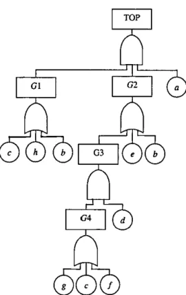
The top-down approach for calculating the mmimal cut sets 1s demonstrated using the example fault tree shown in Figure 2 1. Startmg w1th the top event (Top) it 1s
F1gure 2 1 Example fault tree
an 'AND' gate w1th three inputs G1, a and G2. It can therefore be expressed as a product of these inputs:
Top= G1 ·a· G2. (2 19)
As G1 IS an 'OR' gate, made up of three events, a, b and c, it can be written as:
G1
=
a+b+c (2 20)Substituting th1s into Top g1ves:
Similarly, G2 can be written as the 'sum' of b and d, so Top becomes
Top= (a+ b +c)· a· (b +d) (2 22)
The expresswn now contams only basic events, so is expanded to give
Top - a · a · b
+
a · a d +a · b · b +a· b · d +a c · b+
a · c · d (2 23)a· b +a· d +a· b +a· b · d+a · c· b+ a· c· d (as a· a= a and b·b= b),
which gives the cut sets of the fault tree. These are simply the cut sets expressed m sum-of-products form. Redundancies can then be removed using the 1dempotent and absorptiOn laws:
Top = a · b
+
a· d (2 24) This is the minimal disjunctive form of the logic equatwn each term of which is a m1mmal cut set. For this fault tree there are two m1mmal cut sets, both of order two (i e. they each contam two basic events). These are{a,
b} and{a,
d}.A complex system may produce thousands of minimal cut sets. Although the algonthm IS not complex the process can be very time-consuming. For this reason approximatiOns are often Implemented which removes the cut sets above a certain order (for example, above order three) durmg the calculatiOn process. Th1s approx-imation reduces the number of computations and the time taken for the analysis However, this obvwusly leads to a reduction m the accuracy of the m1mmal cut sets and therefore in the resulting quantitative analysis for wh1ch mimmal cut sets are reqmred.
2.4 Quantitative Analysis
Quantitative analysis of the fault tree allows the calculation of a number of param-eters which are used to assess the system The top event probabrlity and frequency are used together wrth the expected number of occurrences of the top event and event importance measures to gain a full understanding of the system.
The methods for fault tree quantificatiOn are known as Kinetrc Tree Theory [1]
whrch rs a time dependent methodology for system evaluatwn This techmque forms the basis of the approach used m the majority of commercial Fault Tree Analysis packages
2.4.1 Structure Functions
The structure functwn is a binary functiOn taking the following values rf>(x)
= {
1 1f the system is fa1led,0 1f the system is workmg, (2.25)
where x
=
(xi> x2 , • , Xn) is an indicator vector showing the status (workmg or failed) of each componentFor each system component, J, the bmary indicator vanable, x3, is presented
{
1 1f component J is fa1led,
XJ
=
0 1f component J is workmg. (2 26)
The structure funct1on for the top event of a fault tree shows the system state m relation to its components and is g1ven by:
N
rf>(x)
=
1-IT
(1-p,(x)), (2.27)~=1
where p,(x) is the bmary indicator functwn for each mimmal cut set K., z
=
1 .N:( ) IT
h h{
1 if cut set K, eXJsts,
p, x
=
x3 sue t at p,=
JEK, 0 if cut set K, does not ex1st
(2 28)
For the fault tree shown m Figure 2 1, wh1ch has minimal cut sets K1 ={a, b} and
K2
=
{a, d}, the structure function is given by:(2 29)
The probab1lity of the top event is given by the expected value of the structure function:
Q(t) = E[rf>(x)J (2 30)
If each minimal cut set is mdependent (i e. no event appears m more than one cut set) then 1t is also true that:
E[rf>(x)]
=
r/>[E(x)J. (2.31)Obtaimng the expected value of the structure function for independent m1mmal cut sets would Simply be a matter of substitutmg the probability of fa1lure of each component mto the structure function and calculatmg the result. However, the
mimmal cut sets are not usually independent, and so in this case a full expansion of the structure functwn and the reduction of the indicator variables (i.e. x,
=
x~)must be undertaken.
Applymg this to the structure function for the example fault tree in Equation 2 29, gives:
<P(x) (2.32)
using expanswn and reduction The probab1hty of the top event IS then g1ven by
the expected value of th1s structure functwn.
Q(t)
=
P(a) · P(d) + P(a) · P(b)- P(a) · P(b) · P(d) (2.33) A more effic1ent method of implementing this uses Shannon's Theorem.2.4.2 Shannon's Theorem
Shannon's Theorem can be expressed as follows A Boolean function f(x) can be wntten as:
f(x)
=
x, · !(1., x)+
x, ·
f(O., x),where
x,
1-x.,!(1., x) and f(O., x) are known as the res1dues of f(x) w1th respect to x,
(2.34)
(2 35)
(2 36)
(2.37)
The structure function is pivoted around the most repeated variable using Shan-non's expansion. This 1s contmued until no repeated vanables exist in the residues
Shannon's theorem can be apphed to the structure function g1ven m Equation 2.29. Pivoting around the repeated variable, a, gives
<P(x) Xa[1 - (1- Xb)(1 - Xd)]
+
(1 - Xa)[O] Xa(1- (1- Xb)(1- Xd))The probability of the top event is therefore g1ven by
Q(t) - E(rp(x)) (2.39)
- P(a)(1- (1- P(b))(1- P(d))).
Expanding th1s gives exactly the same result shown in Equatwn 2 33.
2.4.3 General Method for the Calculation of the Top Event
Probability
Th1s general method of calculating the top event probability (i e. the system un-availability) uses the minimal cut sets obtained from the qualitative analysis [4]. This method can be used whether or not the fault tree contams repeated events
The top event occurs 1f at least one mmimal cut set exists, therefore for a fault tree that has N m1mmal cut sets, K., Q(t) is g1ven by:
N Q(t) = P(U K,). (2 40) t=l Expandmg g1ves. N N •-1 Q(t) LP(K,)- LLP(K,nK3)+ (2.41) t=l t=2 J=l
where P(K,) IS the probability of the eXIstence of m1mmal cut set z.
This expanswn IS known as the mcluswn-exclusion expansiOn and generates the exact probability of the top event existence Consider the example fault tree shown m Figure 2.1, wh1ch has mimmal cut sets K1
=
{a,b} and K2=
{a,d}Equation 2 41 g1ves the top event probability as:
Q(t) - P(K1)
+
P(K2)- P(K1n
K2) (2 42)= P(a) · P(b)
+
P(a) P(d)- P(a). P(b). P(d), which is ident1cal to the expression calculated m Equation 2.33.It IS usual to have fault trees for engineermg systems which result m tens of thou-sands of mimmal cut sets Therefore it is impractical m these Situations to calculate all terms in the complete expanswn. For th1s reason the calculation 1s simplified by the use of approximations
2.4.3.1 Upper and lower bounds for system unavailability
Truncation of the senes m Equation 2 41 at an even-numbered term gives a lower bound for the top event probability, truncatiOn at an odd-numbered term gives an upper bound for the top event probability
N N t-! N
LP(K,)- LLP(K, nK1 ):::; Q(t):::; LP(K,). (2.43) ~=1 t=2 J=l t=l
The upper bound IS known as the Rare Event Approximation, PRE(Top), as It IS accurate 1f the component failure events are rare
N
PRE(Top)
=
L P(K,) (2 44)t=l
2.4.3.2 Minimal cut set upper bound
A more accurate upper bound is Minimal Cut Set Upper Bound, PMcsus(Top). Th1s IS derived as follows
P(system failure)
Also,
P(at least one m1mmal cut set exists)
- 1-P(no m1mmal cut sets exist).
N
(2 45)
P(no mimmal cut sets exist):::::
IT
P(mmimal cut set z does not exist). (2.46)t=l
Equality exists when no event occurs in more than one cut set.
Substituting Equation 2 46 mto Equation 2 45 g1ves
N
P(system failure) :::; 1-
IT
?(minimal cut set z does not exist), (2 47)t=l
which gives the Minimal Cut Set Upper Bound
N
PMcsus(Top)
=
1-IT
(1- P(K,)). (2 48)t=l
It can be shown that
N N
Q(t) :::; 1-
IT
(1- P(K,)) :::;L
P(K,). (2 49)2.4.4
Top
Event Frequency
The top event frequency IS another system parameter that can be calculated -this is useful for systems where unreliabihty IS an Important issue. The system unconditional failure intensity, Wsys(t), is defined as the expected number of times the top event occurs at time t, per umt time Therefore Wsys(t)dt is the expected number of times the top event occurs in t to t
+
dt For the top event to occur in the mterval[t,
t+
dt) none of the cut set failures can exist at timet,
and then at least one of them must fail m time t to t+
dt. This can be wntten as:N
Wsys(t)dt
= P(A
U
0,), (2 50)t=l
where·
A is the event that no m1mmal cut sets exist at time t,
u:l
e,
is the event that one or more mmimal cut sets occur in time[t,
t+
dt)As P(A)
=
1 - P(A), the nght hand of EquatiOn 2.50 can be wntten·N N N
P(A
U
e,)
=P(U
e,) -
P(AU
e,),
(2 51)t=l t=l t=l
where A is the event that at least one mimmal cut set exists at t.
Therefore Wsys(t) becomes·
N N
Wsys(t)dt
=
P(U
e,)-
P(Au
e,).
(2.52)t=l t=l
The first term on the right-hand s1de gives the contnbution from the occurrence of at least one m1mmal cut set. The second term gives the contribution of the m1mmal cut set occurrence while other mmimal cut sets already exist (1 e. the system is already failed) These terms are denoted by w~Vs(t)dt and w~V.(t)dt respectively to g1ve:
(2.53)
The terms on the nght of the above equation can be expanded usmg the inclusiOn-exclusiOn prmCiple but as this is a computationally mtensive operatiOn, an approx-imatiOn is required
2.4.4.1 Approximation for the system unconditional failure intensity
If component failures are rare then mimmal cut set fmlures will also be rare events. The term
wiV.(t),
which requires m1mmal cut sets to ex1st and occur at the same t1me, would become negligible 1f component fa1lures are unlikely Therefore, an upper bound for Wsys(t) IS Simply:(2 54)
As Wsys(t) can be expanded using the mclusion-excluswn pnnciple the series ex-pansiOn is truncated after the first term (as for the top event probability) to give the Rare Event Approximation:
N N
Wsys(t)maxdt:::::
L
P(B,) ::=;L
WK,(t)dt, (2.55)•=I k=l
where
WK, (t) is the unconditiOnal fa1lure intens1ty of mmimal cut set K,
2.4.4.2 Expected number of system failures
The expected number of system fmlures m timet, W(O, t), is given by the mtegral of the system unconditional fa1lure intensity m the mterval t:
W(O,t)= lWsys(u)du (2 56)
For a rehable system the expected number of system fa1lures is an upper bound for the system unrehab1hty, F(t) (i e. F(t) ::::: W(O, t)).
2.4.5 Importance Measures
A very useful piece of mformation which can be denved from a system rehab1hty assessment IS the importance measure for each component or minimal cut set. An importance analys1s is a sensitivity analys1s which identifies weak areas of the system and can be very valuable at the design stage For each component its importance s1gmfies the role that it plays m either causmg or contnbuting to the occurrence of the top event. In general a numerical value IS ass1gned to each basic event which allows it to be ranked accordmg to the extent of 1ts contnbution to the occurrence of the top event. Importance measures can be categonzed m two ways: determm1st1c and probabJhst1c
2.4.5.1 Deterministic measures
Determimstic importance measures evaluate the importance of a component
with-out considering its probability to fa1!. One such measure IS Structural Measure of
Importance It is given by·
I _ number of cntical system states for component z
' - total number of states for the ( n - 1) remaining components (2 57)
A critical system state for component z is a state for wh1ch the failure of component z will cause the system to go from a workmg to a fa1led state.
2.4.5.2 Probabilistic measures of system unavailability
Probab1listic measures are generally of more use than deterministic measures m re-liability problems as they take mto account the components' probability of fa1lure
Bzrnbaum's Measure of Importance IS also known as the criticality functiOn which defines the probability that the system is m a cnt1cal system state for component z. There are two expressiOns which can be used to obtam the criticality function
a)
G,(q(t))
=
Q(1., q(t))- Q(O., q(t)),(2
58)where
Q( t) IS the probability that the system fmls,
(1., q(t))
=
(q~o ., q,_l> 1, q,+l>. , qn) component z failed, (0., q(t))=
(q~o ... , q,_l, 0, qt+l> , qn) component z is workmg.The above expresswn gives the probability that the system fails with component z failed minus the probability of the system fa1ling with component z workmg, which results in the probability that the system fa1ls only 1f component z fails.
b) 8Q(t)
G,(q(t))
=
8q,(t). (2 59)This is eqmvalent to Equatwn 2 58 as the probability functwn IS lmear m each
q,(t)
8Q(t) Q(1., q(t))- Q(O., q(t))
-8q,(t) 1- 0 (2 60)
In terms of Birnbaum's measure of component reliability importance, the expected number of system fa1lures can be calculated as.
rt
nW(O,t)
=
Jn LG,(q(t))w,(u)du,0 t=l
(2 61)
where w,(t) denotes the component unconditional fa1lure intens1ty and n denotes the total number of system components.
Cntzcalzty Measure of Importance calculates the probability that the system IS in a cnt1cal state for component z and that z has failed Unlike Birnbaum's mea-sure of Importance 1t also takes mto account the fa1lure probab11ity of component z 1tself·
I _ G,(q(t))q,(t)
' - Q(t) (2 62)
Pussell- Vesely Measure of Importance calculates the probability that component z contnbutes to system fa1lure and IS defined as the probability of the union of the mmimal cut sets contaimng z, g1ven that the system has fa1led ·
I - P(UJI•EK, KJ)
' - Q(t) (2.63)
Th1s measure gives very s1milar importance rankings to those obtained usmg the cntlcality measure.
Pussell- Vesely Measure of Mznzmal Cut Set Importance ranks the minimal cut sets in the order of their contnbutwn to the top event, rather than cons1dering the mdividual components. It is defined as the probab1lity of ex1stence of the cut set z, given that the system has failed
P(K,)
I,= Q(t) .
2.5 Simplification of the Fault Tree Structure
(2 64)
Fault trees can be very large and the1r qualitative and quantitative analyses time-consuming. Therefore two pre-processing techniques can be applied to the fault tree m order to obtain the smallest possible subtrees [5] The first stage of pre-processmg is a reductiOn, techmque used m the Faunet code [6], winch restructures the fault tree to 1ts most conc1se form. Once th1s has been applied it is poss1ble to
simplify the analysis further by 1dentJfymg mdependent subtrees (modules) w1thin the fault tree that can be treated separately The Rauzy's algorithm [7] is an extremely efficient method of modulansation and forms the second stage of fault tree pre-processmg. This results m a set of independent fault trees each with the simplest possible structure, wh1ch together descnbe the onginal system
2.5.1 Fault Tree Reduction
The reduction technique reduces the fault tree to its minimal form so eliminating any 'noise' from the system without altermg the underlying logic
2.5.1.1 Introduction
Fault trees are rarely written m their most concise format and th1s can have a significant effect on the efficiency of the resultmg analysis The1r complexity can be reduced by applymg fault tree reduction techniques, wh1ch optimise the structure of the tree wh1lst retaining the underlymg logic One such technique is the reductwn approach, wh1ch IS applied in four stages
2.5.1.1.1 Reduction technique
This method of fault tree reduction cons1sts of four stages.
1. Contraction
Subsequent gates of the same type are contracted to form a smgle gate. This g1ves an alternatmg sequence of 'AND' gates and 'OR' gates throughout the tree
2 FactorisatiOn
Pairs of events that always occur together m the same gate type are 1denhfied. They are combmed to form a single complex event.
3 Extraction
The two structures shown in Figure 2 2 are 1dent1fied and replaced as shown
4. Absorption
The structures m the fault tree are identified that could be further s1m plified through the application of the absorptiOn and idem potent laws to the fault tree logic. If primary and secondary gates with an event in common are of a different type, the structure is simplified by removmg the whole secondary
gate and 1ts descendants. If pnmary and secondary gates are of the same type, the structure is simplified by deleting the occurrence of the event beneath the secondary gate. These cases are illustrated in Ftgure 2.3
Ftgure 2.2: The extractiOn procedure
Pnmary-
0
0
+-Pnmaryfun>~
+0
0
Pnm~y
g~e ~
-0
gate gate~
-6
~
+-gateSecondary
-£
Secondary-+£
9
+-Secondary~ ~ ~
b
a b a b
Ftgure 2 3 The absorptiOn procedure
The above four steps are repeated until no further changes are possible in the fault tree, resulting m a more compact representation of the system.
2.5.1.2 Worked example of the reduction technique
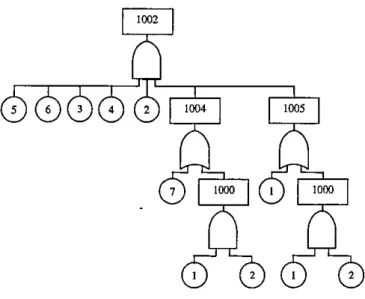
Thts technique wtll be applied to the example fault tree It IS shown m Ftgure 2 4
Figure 2.4· Example of fault tree
2.5.1.2.1 Contraction
The aim of the first stage is to ident1fy subsequent gates m the tree structure that have the same gate type ApplicatiOn of the contraction stage is implemented to the fault tree shown m F1gure 2.4.
In this example gate 1003 appears as an mput to gate 1002 and they both are 'AND' gates Gate 1003 only appears once m the fault tree data, so 1ts inputs are directed to gate 1002. Since gate 1004 IS an input to gate 1002 1t is not listed for
the second t1me. Now gate 1001 appears as an input to gate 1002 and they are both 'AND' gates As gate 1001 only appears once in the fault tree data, its inputs are d1rected to gate 1002 The resultmg fault tree is shown in Figure 2.5.
2.5.1.2.2 Factorisation
The fault tree now has an alternating sequence of 'AND' and 'OR' gates and can be factonsed. The input events to each gate are considered one by one, lookmg for pairs that always occur together. Once it has been established that they do always occur together and under the same gate type, a complex event IS created, whJCh
is numbered from 2000 upwards. The new complex event is recorded together w1th the gate type and the two events from which it was formed Applicatwn of factorisation to the fault tree shown m Figure 2.5 g1ves complex events listed m Table 2.3. The modified fault tree is shown in F1gure 2.6.
Figure 2.5: The fault tree after contraction
Complex
Gate value Event I Event2 event
2000 AND a b
2001 AND 2000 d
2002 AND 2001 e
Table 2 3. Complex event data after factorisatiOn
2.5.1.2.3 Extraction
The extractiOn process searches for the structures shown m Figure 2 2 If the pn-mary gate has two or more gates as inputs (referred to as the secondary gates) then the gates are selected in pairs. Both secondary gates are then checked to see 1f they are of the same type, but of a d1fferent type to the primary gate If so, the mputs to the secondary gates are checked to see 1f they have a gate or event in common If they do then extraction can take place.
Before extraction can occur, however, there may be some necessary adjustments to be made to the data If the primary gate has more than two m puts then a new gate must be created which has the same gate type as the primary gate, but wh1ch has the primary gate and all its inputs, except the two secondary gates, as mputs. This restructures the fault tree into the form required for extractiOn by usmg an equivalent representation. Application of the extractwn procedure IS carried out
on the fault tree shown in F1gure 2 6
The only gate that has two or more gates as inputs IS top gate 1002, whose inputs
are 1004 and 1005 These secondary gates are both of a different type to the pri-mary gate, and have gate 1000 in common, which can be extracted. In order to get th1s tree into the reqmred form for extractiOn gate 1006 IS generated, as shown
in Figure 2. 7. Gate 1002 now only has its two secondary gates as inputs.
A new gate, 1007, is created, wh1ch is of the same type as the secondary gates and has the same common input, 1000, and the primary gate 1002, as 1ts inputs. The resulting tree is shown in F1gure 2 8
It 1s clear from F1gure 2.8 that another extraction can also be undertaken. Gates
1000 and 1002 also have event 1 in common, wh1ch can be extracted. Since gate
1006 is the same type as the secondary gates, the same common input 1 and the primary gate 1007 are added to the hst of its inputs The fault tree after the extraction IS showed in Figure 2 9.
2.5.1.2.4 Absorption
Durmg the absorptiOn process the repeated events are considered m the fault tree If the type of the pnmary gate IS different from the type of the secondary gate,
F1gure 2.7: The fault tree dunng extraction, gate 1006 IS created
the secondary gate 1s deleted If the types of the primary and secondary gates are the same, the repeated event IS deleted from the list of the m puts of the secondary
gate. ApplicatiOn of the absorption procedure is earned out on the fault tree shown m F1gure 2.9.
The only repeated event m the fault tree is event 2. The first time it occurs as an input to the primary gate 1006, wh1ch IS an 'AND' gate, and the second time
1t occurs as an input to the secondary gate 1007, which IS an 'OR' gate Since the
types of the primary and the secondary gates are different the secondary gate can be deleted. The fault tree after the absorptiOn IS shown in Figure 2 10
Fmally, the factorisatiOn can be applied agam and it fimshes the reductwn process New complex events are shown in Table 2.4. The reduced fault tree is shown m F1gure 2.11 in terms of ongmal gate name and complex event.
F1gure 2 8· The fault tree durmg extraction, gate 1007 IS created
Complex
Gate value Event I Event 2 event
2003 AND 2002 f
2004 AND 2003 !i
Table 2 4. Complex event data after the second factorisation
2.5.1.3 Reduced fault tree
It can be venfied that the reduced tree IS equivalent to the original tree by
exam-ining the1r minimal cut sets. These w111 be identical for logically equivalent trees. The ongmal tree has one m1mmal cut set of order 6
{!,a,
d, b, g,e}.
(2 65)The minimal cut set for the reduced tree is
{2004}. (2.66)
This can be expanded out in terms of the basic events The principle is that 'OR' gates mcrease the number of cut sets, whilst 'AND' gates mcrease the number of elements in the cut sets Therefore the mimmal cut set of the reduced tree can be expanded to give:
TOP - 2004
=
2003 · g=
2002f ·
g=
2001· e ·f ·
g= 2000 d e ·
f ·
g =a· b · d · e ·f ·
g,F1gure 2 9 Fault tree after extraction
F1gure 2.10: Fault tree after absorption
F1gure 2.11: The reduced fault tree
which IS equivalent to those obtamed from the ongmal tree.
ReductiOn has s1mphfied the example fault tree considerably. In the original fault tree there were six gates and fourteen events, e1ght of them different; the reduced fault tree contains one event However, th1s method rarely reduces a fault tree to a single event as 1t d1d m this simple example
Having reduced the fault tree to a more conc1se form the second pre-processing technique of modulansation is considered.
2.5.2 Fault 'free Modularisation
Modulansation methods can be applied to fault trees in order to reduce their com-plexity and simplify the resultmg analys1s The modularisation procedure 1dentilies subtrees within the fault tree, known as modules. A module of a fault tree 1s a subtree that is completely mdependent from the rest of the tree. It contains no bas1c events that appear elsewhere in the fault tree The advantage of ident1fying these modules is that each one can be analysed separately from the rest of the tree The results from subtrees identified as modules are substituted into the higher-level fault trees where the modules occur
Several modulansation techniques are available for detecting fault tree modules but one of particular interest IS Rauzy's linear-time algonthm [7]. The advantage of th1s algonthm over other techniques is its efficiency, only two passes through the fault tree are required m order to obtain the modules.
2.5.2.1 Rauzy's algorithm
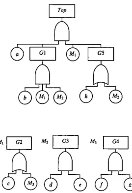
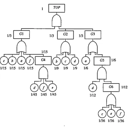
Usmg the lmear-t1me algonthm the modules can be identified after JUSt two depth-first traversals of the fault tree. The depth-first of these performs a step-by-step traversal recordmg, for each gate and event, the step number at the first, second and final vis-Its to that node To demonstrate this process refer to the fault tree in F1gure 2.12.
Starting at the top event and progressing through the tree m a depth-first manner the gates and events are vis1ted in the order shown m Table 2.5.
Step number 1 2 3 4 5 6 7 8 9 10 11 12 13
node Top a Gl b G2 c
G4
f
gG4
G2G3
dStep number 14 15 16 17 18 19 20 21 22
node e
G3
G1 G2 G5 hG3
G5 TopTable 2 5: Order m which the gates and events are visited m the depth-first traver-sal of the fault tree in F1gure 2.12
Event mputs to any gate are cons1dered before the gate inputs. Each gate is VIS-Ited at least tw1ce. once on the way down the tree and again on the way back up the tree. Once a gate has been visited 1t can be vis1ted agam, but the depth-first traversal beneath that gate is not repeated This 1s shown at step 17 and step
Figure 2.12. Example fault tree to demonstrate the linear-time algonthm
events appearmg below that gate in the tree) are not re-v1S1ted. The step numbers of the v1sits (first, second and final) are recorded during this traversal and values for the gates are shown m Table 2 6.
Gate Top G1 G2 G3 G4 G5 pt vis1t 1 3 5 12 7 18 2nd VISit 22 16 11 15 10 21 Final visit 22 16 17 20 10 21 M in 2 4 6 13 8 12 Max 21 17 10 14 9 20
Table 2.6· Data for the gates in the fault tree
As gates G2 and G3 are repeated gates the step numbers of the final VISit are different to those of the second visit. The equivalent data for the events is shown in Table 2. 7. It should be noted that the step number of the second visit to each basic event is equivalent to the step number of the first v1sit to that event
The second pass through the tree finds the max1mum (max) of the last visits and the mmimum (mm) of the first vis1ts to the descendants of each gate, these values are also shown m Table 2 6
Event a b c d e
f
g h pt VISit 2 4 6 13 14 8 9 192nd VISit 2 4 6 13 14 8 9 19
Fmal vis1t 2 4 6 13 14 8 9 19
Table 2. 7. Data for the events m the fault tree
The prmc1ple of the algorithm is that 1f any descendants of each gate has a first vis1t step number smaller than the first visit step number of the gate then 1t must occur beneath another gate. Conversely, if any descendant has a last visit step number greater than the second visit step number of the gate, then agam it must occur elsewhere in the tree.
Therefore, a gate can be identified as headmg a module 1f
• The first visit to each descendant is after the first v1sit to the gate, • The last visit to each descendant is before the second VISit to the gate. That 1s, none of the descendants of a gate can appear anywhere else m the tree (unless beneath another occurrence of the same gate). Therefore, the final step of the algonthm simply compares the minimum (min) and mrunmum (max) values of the descendants visit numbers w1th the first and second v1sit step numbers for each gate.
From Table 2.6 it can be seen that gate Gl cannot be a module as 1ts descen-dants have a maximum step number greater than the second VISit step number of th1s gate Gate G5 IS also not a module as 1ts descendants have a mimmum step number smaller than the first visit step number of the gate
The following gates can therefore be identified as headmg modules
Top, G2, G3, G4. (2 68)
The top event w1ll always be a module of the fault tree Each of the subtrees can be replaced by a smgle modular event in the fault tree structure and are assigned the followmg labels
Four separate fault trees as shown in Figure 2 13 now replace the single tree shown m Figure 2 12
Figure 2 13 The four modules obtained from the fault tree shown m Figure 2.12 - Modulansed fault tree, Module M1, Module M2 and Module M3
Having identified the modules each one can be analysed separately into the higher-level fault trees where the modules occur. This process can sigmficantly reduce the number of calculatiOns reqmred in the subsequent analysis.
2.6 Summary
Fault Trees are an extremely good way of representing the fmlure logic of the system in a visual format. The qualitative analysis enables minimal cut sets of the tree to be found, which are the smallest combmations of basic events that cause system failure. A number of parameters, such as the top event probability and frequency, together with the expected number of occurrences of the top event and event importance measures, obtained from the quantitative analysis gam a full understandmg of the system But this analysis has a disadvantage - if the fault tree IS large then performing analysis upon it can reqmre extensive calculatiOns.