MIXED INTEGER PROGRAMMING APPROACHES FOR NONLINEAR AND STOCHASTIC PROGRAMMING
A Thesis Presented to The Academic Faculty
by
Juan Pablo Vielma Centeno
In Partial Fulfillment of the Requirements for the Degree
Doctor of Philosophy in the
School of Industrial and Systems Engineering
Georgia Institute of Technology August 2009
MIXED INTEGER PROGRAMMING APPROACHES FOR NONLINEAR AND STOCHASTIC PROGRAMMING
Approved by:
Professor George Nemhauser, Advisor School of Industrial and Systems Engineering
Georgia Institute of Technology
Dr. Zonghao Gu Gurobi Optimization
Professor Shabbir Ahmed, Advisor School of Industrial and Systems Engineering
Georgia Institute of Technology
Professor Ellis Johnson
School of Industrial and Systems Engineering
Georgia Institute of Technology Professor William J. Cook
School of Industrial and Systems Engineering
Georgia Institute of Technology
To my wife Johana, and my mother Mar´ıa Ang´elica.
ACKNOWLEDGEMENTS
I would like to thank my advisors Prof. George L. Nemhauser and Prof. Shabbir Ahmed for their support throughout my PhD. I am extremely grateful for their advice, guidance and inspiration in my research and career. Thanks also to the remaining member of my committee Professor William J. Cook, Dr. Zonghao Gu and Professor Ellis Johnson.
I would specially like to thank my wife and parents for their unconditional love and constant encouragement. I am deeply appreciate all the sacrifices they did to support me over many years of study.
I would also like to thank the faculty and staff of the H. Milton Stewart School of Industrial and Systems Engineering for the high quality education I received during my PhD. I would specially like to thank my fellow students and friends for helping make the time I spent at Georgia Tech some of the best years of my life.
Finally, I would like to acknowledge the partial support for this research from National Science Foundation grants DMI-0121495, DMI-0522485, DMI-0133943, CMMI-0522485 and CMMI-0758234, AFOSR grant FA9550-07-1-0177, a grant from Exxon Mobil Upstream Re-search Company and the John Morris Fellowship from the Georgia Institute of Technology.
TABLE OF CONTENTS
DEDICATION . . . iii
ACKNOWLEDGEMENTS . . . iv
LIST OF TABLES . . . viii
LIST OF FIGURES . . . x
SUMMARY . . . xi
I INTRODUCTION . . . 1
1.1 Background . . . 1
1.1.1 LP based solvers . . . 1
1.1.2 Modeling with MILP . . . 3
1.2 Dissertation Overview . . . 10
II A LIFTED LINEAR PROGRAMMING BRANCH-AND-BOUND ALGORITHM FOR MIXED INTEGER CONIC QUADRATIC PROGRAMS . . . 13
2.1 Introduction . . . 13
2.2 A Branch-and-Bound Algorithm for Convex MINLP . . . 17
2.3 Lifted Polyhedral Relaxations . . . 21
2.4 Computational Results . . . 24
2.4.1 Implementation . . . 25
2.4.2 Test Instances . . . 25
2.4.3 Results . . . 27
2.5 Conclusions and Further Work . . . 39
III MODELING DISJUNCTIVE CONSTRAINTS WITH A LOGARITHMIC NUM-BER OF BINARY VARIABLES AND CONSTRAINTS . . . 41
3.1 Introduction . . . 41
3.2 Modeling a Class of Hard Combinatorial Constraints . . . 43
3.3 Branching and Logarithmic Size Formulations . . . 48
3.4 Modeling Nonseparable Piecewise Linear Functions . . . 52
3.5 Extension of the Model to Ground Set [0,1]J . . . . 57
3.7 Conclusions . . . 65
IV MIXED-INTEGER MODELS FOR NONSEPARABLE PIECEWISE LINEAR OPTIMIZATION: UNIFYING FRAMEWORK AND EXTENSIONS . . . 67
4.1 Introduction . . . 67
4.2 Modeling Piecewise Linear Functions . . . 68
4.3 Mixed Integer Programming Models for Piecewise Linear Functions . . . 71
4.3.1 Disaggregated convex combination models . . . 71
4.3.2 Convex combination models . . . 73
4.3.3 Multiple choice model . . . 76
4.3.4 Incremental model . . . 77
4.4 Properties of Mixed Integer Programming Formulations . . . 78
4.5 Computational Experiments for Continuous Functions . . . 83
4.5.1 Continuous Separable Concave Functions . . . 83
4.5.2 Continuous Non-Separable Functions . . . 89
4.6 Extension to Lower Semicontinuous Functions . . . 92
4.6.1 Formulations with Direct Extension . . . 94
4.6.2 Ad-Hoc Extension for Univariate Functions . . . 95
4.6.3 Theoretical Properties of Formulations . . . 100
4.7 Computational Experiments for Lower Semicontinuous Functions . . . 101
4.7.1 Discontinuous Separable Functions . . . 101
4.7.2 Discontinuous Non-Separable Functions . . . 104
4.8 Conclusions . . . 105
V MIXED INTER LINEAR PROGRAMMING FORMULATIONS FOR LINEAR PROGRAMMING WITH PROBABILISTIC CONSTRAINTS . . . 107
5.1 Introduction . . . 107
5.2 Existing MILP Formulations . . . 108
5.2.1 1-row Relaxation . . . 109
5.2.2 Extended 1-row Formulation . . . 111
5.2.3 Blending . . . 114
5.3 Extended Formulation for d >1 . . . 114
5.4.1 Negative results . . . 118
5.4.2 Positive Results . . . 123
5.5 Computational Results . . . 129
5.5.1 Sharpness Testsd= 2 . . . 130
5.5.2 Interaction with Other Constraints . . . 133
5.6 Conclusions . . . 137
LIST OF TABLES
1 Problem Sizes for Different Values of ε . . . 28
2 Number of Nodes for Different Values of ε . . . 29
3 Solve Time for Different Values ofε[s] . . . 29
4 Number of Nodes that SolveCPP(lk, uk) . . . 29
5 Solve Times for Small Instances [s] . . . 32
6 Solve Times for Medium Instances [s] . . . 33
7 Solve Times for Large Instances [s] . . . 35
8 Solve Time for Root Relaxation [s] . . . 36
9 Accuracy of RelaxationzLP(ε) [%] . . . 37
10 Problem Sizes for Different Values of n . . . 37
11 Total Number of Nodes and Calls to Relaxations for All Instances . . . 38
12 Total Number of Nodes and Calls to Relaxations for Small Instances . . . . 39
13 Solve times for one variable functions [s]. . . 63
14 Solve times for two variable functions on a 4×4, 8×8 and 16×16 grids [s]. 65 15 Sizes of Formulations . . . 82
16 Solve times for univariate continuous functions [s]. . . 85
17 Solve characteristics for univariate continuous functions andK = 4. . . 87
18 Solve characteristics for univariate continuous functions andK = 8. . . 87
19 Solve characteristics for univariate continuous functions andK = 16. . . 88
20 Solve characteristics for univariate continuous functions andK = 32. . . 89
21 Solve times for two variable multi-commodity transportation problems. [s]. 91 22 Solve times for univariate discontinuous functions [s]. . . 103
23 Solve times for non-separable functions [s]. . . 105
24 Marginal GAP for d= 2 [%]. . . 132
25 1-row GAP for d= 2 [%]. . . 133
26 Transportation Problems 1-row GAP for d= 2 [%]. . . 135
27 Transportation Problem 2-row GAP for d= 2 [%]. . . 136
28 Marginal GAP for d= 4 [%]. . . 137
30 2-row GAP for d= 4 [%]. . . 139 31 Transportation Problem 1-row GAP for d= 4 [%] . . . 140 32 Transportation Problem 2-row GAP ford= 4 [%] . . . 141
LIST OF FIGURES
1 Basic LP Based Branch-and-Bound Algorithm. . . 2
2 Univariate Interpolated Piecewise Linear Function. . . 8
3 Interpolating Bivariate Functions. . . 9
4 A Lifted LP Branch-and-Bound Algorithm. . . 19
5 Performance Profile for Different Values of ε. . . 30
6 Performance Profile for Small Instances . . . 31
7 Performance Profile for Medium Instances . . . 34
8 Performance Profile for Large Instances . . . 36
9 Two level binary trees for example 3.3. . . 49
10 Triangulations . . . 53
11 Partial B&B tree for Example 3.6 . . . 56
12 A continuous piecewise linear function and its epigraph as the union of poly-hedra. . . 69
13 Examples of triangulations of subsets of R2. . . 76
14 Lower semicontinuous piecewise linear functions. . . 92
15 Decomposition of fixed charged lower semicontinuous piecewise linear function. 98 16 Example 5.1. . . 110
17 Example 5.3 for L= 0. . . 119
18 Example 5.5. . . 123
19 Simple Configuration. . . 124
20 Cases of Proposition 5.3. . . 128
21 Integers in box for d= 2,M1 = 13,M2 = 9 and δ= 0.4. . . 129
SUMMARY
In this thesis we study how to solve some nonconvex optimization problems by using methods that capitalize on the success of Linear Programming (LP) based solvers for Mixed Integer Linear Programming (MILP). A common aspect of our solution approaches is the use, development and analysis of small but strong extended LP/MILP formulations and approximations.
In the first part of this work we develop an LP based branch-and-bound algorithm for mixed integer conic quadratic programs. The algorithm is based on a higher dimensional or lifted polyhedral relaxation of conic quadratic constraints introduced by Ben-Tal and Ne-mirovski. The algorithm is different from other LP based branch-and-bound algorithms for mixed integer nonlinear programs in that, it is not based on cuts from gradient inequalities and it sometimes branches on integer feasible solutions. We test the algorithm on a series of portfolio optimization problems and show that it significantly outperforms commercial and open source solvers based on both linear and nonlinear relaxations.
In the second part we study the modeling of a class of disjunctive constraints with a logarithmic number of binary variables and constraints. Many combinatorial constraints over continuous variables such as SOS1 and SOS2 constraints can be interpreted as disjunc-tive constraints that restrict the variables to lie in the union of a finite number of specially structured polyhedra. Known mixed integer formulations for these constraints have a num-ber of binary variables and extra constraints linear in the numnum-ber of polyhedra. We give sufficient conditions for constructing formulations for these constraints with a number of binary variables and extra constraints logarithmic in the number of polyhedra. Using these conditions we introduce mixed integer binary formulations for SOS1 and SOS2 constraints that have a number of binary variables and extra constraints logarithmic in the number of continuous variables. We also introduce the first mixed integer binary formulations for piecewise linear functions of one and two variables that use a number of binary variables and
extra constraints logarithmic in the number of linear pieces of the functions. We prove that the new formulations for piecewise linear functions have favorable tightness properties and present computational results showing that they can significantly outperform other mixed integer binary formulations.
In the third part we study the modeling of non-convex piecewise linear functions as MILPs. We review several new and existing MILP formulations for continuous piecewise linear functions with special attention paid to multivariate non-separable functions. We compare these formulations with respect to their theoretical properties and their relative computational performance. In addition, we study the extension of these formulations to lower semicontinuous piecewise linear functions.
Finally, in the fourth part we study the strength of MILP formulations for LPs with Probabilistic Constraints. We first study the strength of existing MILP formulations that only considers one row of the probabilistic constraint at a time. We then introduce an extended formulation that considers more than one row of the constraint at a time and use it to computationally compare the relative strength between formulations that consider one and two rows at a time.
CHAPTER I
INTRODUCTION
1.1 Background
A Mixed Integer Linear Programming (MILP) problem is a nonconvex optimization problem given by
zMILPP:= max cx+dy (1a)
s.t.
Dx+Ey≤f (1b)
y∈Rp (1c)
x∈Zn (1d)
where R is the set of real numbers, Z is the set of integers, c ∈ Rn, d∈ Rp, D ∈ Rm×n,
E ∈Rm×p and f ∈ Rm. We denote this problem by MILPP and say a solution (˜x,y) is˜
feasible forMILPPif it satisfies constraints (1b)–(1d).
In its 50+ years of history, MILP theory and algorithms have been significantly devel-oped [22, 52, 58, 80, 104, 115, 141] and MILP is now considered standard practice in many applications areas (e.g. [20, 47, 57, 76, 96, 106, 107, 129, 135]). Two reasons for the success of MILP are its modeling flexibility [40, 67, 139] and the effectiveness of state of the art Linear Programming (LP) based solvers [24, 25, 69].
1.1.1 LP based solvers
LP based solvers for MILP rely heavily on the LP relaxation ofMILPPgiven by (1a)–(1c),
which we denote by LPP. The basis for these solvers is the Branch-and-Bound algorithm
[77] that performs an intelligent enumeration of the feasible solutions toMILPPby solving a
series of LP problems based onLPP. The simplest version of this algorithm can be described
as follows. For any (lk, uk) ∈(
Z∪ {−∞})n×(Z∪ {+∞})n we denote by LPP(lk, uk) and MILPP(lk, uk) the problem obtained by adding constraintslk≤x≤uk toLPPand MILPP
respectively. We also denote by zLPP(lk,uk) and zMILPP(lk,uk) the optimal objective value of LPP(lk, uk) and MILPP(lk, uk). In addition, we say that a solution (˜x,y) feasible for˜ LPP(lk, uk) is integer feasible if it is also feasible for MILPP. A branch-and-bound nodek
is defined by some (lk, uk,UBk)∈
Z2n×(R∪ {+∞}) where (lk, uk) are the bounds defining
the node and UBk is an upper bound onz
MILPP(lk,uk). Finally, we denote by LB the global lower bound on zMILPP and by H the set of active branch-and-bound nodes. With these
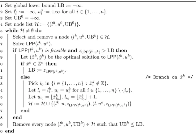
definitions the basic branch-and-bound algorithm is given by the pseudocode in Figure 1 Set global lower bound LB :=−∞.
1 Set l0 i :=−∞,u0i := +∞ for alli∈ {1, . . . , n}. 2 Set UB0 = +∞. 3
Set node listH:={(l0, u0,UB0)}.
4
while H 6=∅do
5
Select and remove a node (lk, uk,UBk)∈ H.
6
SolveLPP(lk, uk). 7
if LPP(lk, uk) is feasible and zLPP(lk,uk)>LB then
8
Let (ˆxk,yˆk) be the optimal solution toLPP(lk, uk).
9 if xˆk∈Zn then 10 LB :=zLPP(lk,uk). 11 else /* Branch on xˆk */ 12 Picki0 in{i∈ {1, . . . , n} : ˆxk i ∈/Z}. 13 Letli =lk i,ui =uki for alli∈ {1, . . . , n} \ {io}. 14 Letui0 =bxˆ k i0c,li0 =bxˆ k i0c+ 1. 15 H:=H ∪ {(lk, u, z LPP(lk,uk)),(l, uk, zLPP(lk,uk))} 16 end 17 end 18
Remove every node (lk, uk,UBk)∈ H such that UBk ≤LB.
19
end
20
Figure 1: Basic LP Based Branch-and-Bound Algorithm.
Lines 8 and 19 of the algorithm eliminate all nodes that cannot have any integer feasible solutions with an objective value larger than that of the best integer feasible solution found so far. If we omit these lines the algorithm will essentially enumerate every ˜x∈Znthat can
be completed to a solution (˜x,y) feasible for˜ MILPP and chose the one for which zLPP(˜x,˜x) is largest. Hence, these steps are crucial for the performance of the algorithm. One of the reasons for effectiveness of modern LP based solvers for MILP is that they use a wide
array of techniques to improve bounds zLPP(lk,uk) in line 8 and UBk in line 19 to a number closer to zMILPP(lk,uk). This is also the reason thatzLPP being close tozMILPP is a desirable property for MILPs.
Another reason for the effectiveness of modern solvers is the use of the warm start capabilities of the simplex algorithm for solving a series of very similar LP problems. For example, LPP(lk, u) constructed in line 16 of the algorithm in Figure 1 is almost identical
toLPP(lk, uk) so we can hope that a few dual simplex iterations starting from the optimal
solution to LPP(lk, uk) would suffice to solveLPP(lk, u). Usually, this is significantly faster
than solvingLPP(lk, u) from scratch.
1.1.2 Modeling with MILP
MILP can clearly be used to model problems where the decision variables are discrete or indivisible such as the number of cars sold or the number of workers assigned to a task. However, MILP can also be used to model additional types of constraints such as implications or other logical conditions. A study of the types of constraints that can be modeled as MILPs began with Meyer [98, 99, 100, 101] and was continued by Jeroslow and Lowe [64, 66, 67, 68, 87]. They showed that the constraints that can be modeled as MILPs are essentially those of the form x∈Si∈IPi ⊂Rn, where {Pi}i∈I is a finite family of polyhedra with a special property that is satisfied if, for instance, all the polyhedra are bounded.
For example, if we wish to model the constraint x∈ Q4 for
Q4 :={x∈R4 : |x1|+|x2| ≤1, x3=x4 = 0} ∪ {x∈R4 : |x2|+|x3| ≤1, x1 =x4= 0}
we can use the MILP formulation given by rx1+sx2 ≤1 ∀r∈ {−1,1}, s∈ {−1,1} (3a) rx2+sx3 ≤1 ∀r∈ {−1,1}, s∈ {−1,1} (3b) rx3+sx4 ≤1 ∀r∈ {−1,1}, s∈ {−1,1} (3c) rx1 ≤z1 ∀r∈ {−1,1} (3d) rx2 ≤z1+z2 ∀r∈ {−1,1} (3e) rx3 ≤z2+z3 ∀r∈ {−1,1} (3f) rx4 ≤z3 ∀r∈ {−1,1} (3g) z1+z2+z3 = 1 (3h) 0≤zj ≤1 ∀j∈ {1,2,3} (3i) z∈Z3 . (3j)
Of course, there are alternative MILP formulations for this constraint, which raises the question of what is a good. One desirable property of the formulation is for its size to be small. However, having the LP relaxation of a MILP be “similar” to the MILP is also a very desirable property. We explore these issues in the next two sections and then give a more practical example of modeling with MILP which is related to two chapters of this thesis.
1.1.2.1 Quality of MILP Formulations If we want to maximize P4
j=1cjxj over all x∈ Q4 for somec∈R4 we can solve the MILP given byzMILPP:= max{
P4
j=1cjxj : (3a)–(3j)}. As noted in Section 1.1.1, the performance of an LP based algorithm when solving this MILP will be highly dependent on how close zLPP := max{
P4
j=1cjxj : (3a)–(3i)} is to zMILPP. Ideally we would like zMILPP = zLPP
or at least δ := (zLPP −zMILPP)/zMILPP 1 for all c ∈ R4. Unfortunately, we have that
δ ≥ 1 for any c ∈ {−1,1}4. In effect, any (x, z) feasible for (3a)–(3j) has P4
j=1|xj| ≤ 1 which implies zMILPP= 1 and, for c∈ {−1,1}4, (x, z) given by xi =ci/2 fori∈ {1, . . . ,4}
achieve zMILPP=zLPP for allc∈R4 by adding to (3a)–(3j) the 16 inequalities given by
4 X i=1
rixi≤1 ∀r ∈ {−1,1}4. (4) The condition zMILPP=zLPP for allc∈R4 is equivalent to asking for the projection of
(3a)–(3i) onto the x variables to be equal to the convex hull of Q4. A MILP formulation with this property is referred to assharp by Jeroslow and Lowe, who also showed that it is the best we can ask from a MILP formulation if we only consider the original x variables [67, 87].
But if we consider the integrality requirements on the z variables of MILPP, there is
an even stronger property. We can ask that every optimal solution to LPP should also be
feasible for MILPP. This property is equivalent to requiring the extreme points of LPPto
naturally comply with the integrality requirements ofMILPP. Whenx∈Si∈IPi is included
in a larger problem that includes additional constraints this property is usually required to hold in the absence of these additional constraint and in this case the formulation is referred to aslocally ideal [105, 106].
A locally ideal formulation is always sharp, but not vice versa. For example, the formulation of x ∈ Q4 given by (3a)–(3j) and (4) is sharp, but its LP relaxation has x1 =x2 = z1 =z3 = 1/2, x3 =x4 =z2 = 0 as an extreme point and hence is not locally ideal.
1.1.2.2 Extended Formulations
Constructing good formulations ofx∈Si∈IPiusing only the originalxvariables and binary variables z ∈ {0,1}|I| can sometimes require a large number of constraints. For example, let Qn be the generalization of Q4 given by
Qn:= n[−1 i=1
A sharp MILP formulation ofx∈ Qn is given by n X j=0 rjxj ≤1 ∀s∈ {−1,1}n (6a) rx1 ≤z1 ∀r∈ {−1,1} (6b) rxj ≤zj+zj−1 ∀i∈ {2, . . . , n−1}, r ∈ {−1,1} (6c) rxn≤zn−1 ∀r∈ {−1,1} (6d) nX−1 j=1 zj = 1 (6e) z∈ {0,1}n−1. (6f)
This formulation has 2n+ 2n+ 1 constraints besides the integrality requirements on z and this number cannot be significantly reduced while preserving the sharpness property if we remain in the (x, z) space. In effect, it is easy to show that constraints (6a) are facet defining for both conv(Qn) and conv (x, z)∈R2n : (6a)–(6f) .
In contrast, if we allow the use of auxiliary variables we can construct formulations with a significantly smaller number of constraints. For example, by using a well known formulation trick we can construct a sharp MILP formulation of x∈ Qn with 4n+ 2 constraints given by rxj ≤yj ∀j∈ {1, . . . , n}, r∈ {−1,1} (7a) n X j=0 yj ≤1 (7b) rx1 ≤z1 ∀r ∈ {−1,1} (7c) rxj ≤zj+zj−1 ∀j∈ {2, . . . , n−1}, r∈ {−1,1} (7d) rxn≤zn−1 ∀r ∈ {−1,1} (7e) n−1 X j=1 zj = 1 (7f) z∈ {0,1}n−1. (7g)
However, this formulation is still not locally ideal for n = 4 since its LP relaxation has x1 =x2 =y1 =y2 =z1 = z3 = 1/2,x3 = x4 =z2 = 0 as an extreme point. Fortunately,
the following theorem by Balas shows us how to construct a locally ideal formulation for a disjunctive set such as Qn.
Theorem 1.1 (Balas [9]). Let D:=
r [ i=1
{x∈Rn : Aix≤bi} (8)
for Ai ∈Rmi×n,bi∈Rmi such that
{x∈Rn : Aix= 0}={x∈Rn : Ajx= 0} ∀i, j ∈ {1, . . . , r}. (9)
A locally ideal formulation with r(n+ 1)variables and r+n+ 1 +Pri=1mi constraints for x∈ D is given by Aixi≤zibi ∀i∈ {1, . . . , r} (10a) r X i=1 xi=x (10b) r X i=1 zi= 1 (10c) z∈ {0,1}r. (10d)
The auxiliary variables used in formulation (10) correspond to a copy of variables xfor each polyhedron on the right hand side of (8) and binary variables that indicate which one of these polyhedrons is selected. Condition (9) simply require that all polyhedrons on the right hand side of (8) should have the same directions of unboundedness.
Using Theorem 1.1 we obtain the locally ideal formulation of x ∈ Qn with 4n−3 variables and 2nconstraints given by
rxj j +sx j j+1≤zj ∀j∈ {1, . . . , n−1}, r∈ {−1,1}, s∈ {−1,1} (11a) x1=x1 1 (11b) xj =xj j+x j−1 j ∀j∈ {2, . . . , n−1}, r∈ {−1,1} (11c) xn=xn−1 n (11d) n−1 X j=1 zj = 1 (11e) z∈ {0,1}n−1. (11f)
MILP formulations that use additional auxiliary variables are usually referred to as ex-tended formulations and have been used to construct strong compact formulations for many problems (for example, see [34] and the references within). The idea of using auxiliary vari-ables to exploit the favorable properties of projection [10] have also been used to construct compact polyhedral approximations of convex sets [15].
1.1.2.3 Example: MILP Models for Piecewise Linear Interpolations
We now show how MILP can be used to model an approximation of a nonlinear function. We first detail the construction for univariate functions and then sketch it for bivariate functions.
A common way to approximate a univariate non-linear function g : [l, u] → R is to
subdivide [l, u] into subintervals of the form [dk−1, dk] for breakpointsl =d0 < d1 < . . . < dK−1 < dK =uand construct the piecewise linear interpolation given by
f(x) :=
g(dk−1) +g(ddkk−)−dg(dk−k1−1)(x−dk−1) x∈[dk−1, dk]. (12) The resulting function f is also referred to as the piecewise Lagrange polynomial of degree 1 or the linear spline interpolation of g (e.g. [102, 110]) and is the only function that is continuous on [l, u], affine on each subinterval [dk−1, dk] and agrees withgon all of the break points. This procedure is illustrated in Figure 2, where gis given by the dashed curve and f by the three thick line segments.
d0 d1 d2 d3 f(d3) 0 f(d0) f(d1) f(d2)
Figure 2: Univariate Interpolated Piecewise Linear Function.
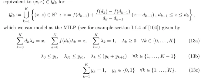
equivalent to (x, z)∈ Qk for Qk:= K [ k=1 (x, z)∈R2 : z=f(dk−1) +f(dk)−f(dk−1) dk−dk−1 (x−dk −1), dk−1≤x≤dk , which we can model as the MILP (see for example section I.1.4 of [104]) given by
K X k=0 dkλk=x, K X k=0 f(dk)λk=z, K X k=0 λk= 1, λk ≥0 ∀k∈ {0, . . . , K} (13a) λ0≤y1, λK ≤yK, λk ≤(yk+yk+1) ∀k∈ {1, . . . , K−1} (13b)
K X k=1
yk= 1, yk∈ {0,1} ∀k∈ {1, . . . , K}. (13c) Constraints (13a) describe (x, z) = (x, f(x)) as the convex combination of points (dk, f(dk))K
k=0. Constraints (13b)–(13c) assures the validity of this convex combination by enforcing the combinatorial requirement on (λk)K
k=0 that at most two λk’s can be non-zero and that if twoλk’s are non-zero their indices must be adjacent (i.e. ifλi >0 andλj >0 thenj =i+1). This combinatorial requirement is known as SOS2 constraints [12].
Formulation (13) is sharp, but it not locally ideal [36, 72, 105]. However, we can again use Corollary 2.1.2 of [9] to get an extended formulation of (x, z)∈ Qk that is locally ideal. This formulation is described in Section 4.3.3 of Chapter 4.
f(x,y)
y
x (a) Bivariate Piecewise Linear Function.
0 1 2 3 4 5 6 7 8 0 1 2 3 4 5 6 7 8 (b) Triangulation
Figure 3: Interpolating Bivariate Functions.
A similar procedure can be used for multivariate functions. For example, for a bivariate function g : [l, u]2 →
finite number of simplices and construct a linear spline interpolation f that is continuous, affine on each of the simplices and agrees with g on all the vertices of the triangulation (e.g. [75]). This procedure is illustrated in Figure 3 where Figure 3(a) shows the piecewise linear function resulting from the interpolation of g(x, y) := sin x/2 + (y/5)2 over the triangulation of [0,8]2 given in Figure 3(b). The vertices of this triangulation are the points in{0,1, . . . ,8}2.
For the resulting piecewise linear function f : [l, u]2 →
R we can use an extension of
formulation (13) for multivariate piecewise linear functions given in [82, 96, 127]. This exten-sion describes (x, y, z) = (x, y, f(x, y)) as the convex combination of points (v1, v2, f(v1, v2)) for each vertex (v1, v2) of the triangulation used to define f. Validity of this convex com-bination is assured by a combinatorial constraint that is the analog of SOS2 constraints for triangulations. This extension is described in detail in Section 3.4 of Chapter 3 and Section 4.3.2 of Chapter 4. This formulation is again sharp and not locally ideal, but we can also use Corollary 2.1.2 of [9] to construct a locally ideal formulation that is described in Section 4.3.3 of Chapter 4.
1.2 Dissertation Overview
In this thesis we study how to solve some nonconvex optimization problems by using meth-ods that capitalize on the success of LP based solvers for MILP. A common aspect of our solution approaches is the use, development and analysis of small but strong extended LP/MILP formulations and approximations.
In Chapter 2 work we develop a LP based branch-and-bound algorithm for Mixed Integer Conic Quadratic programs (MICQP). The algorithm is based on an extended or lifted polyhedral relaxation of conic quadratic constraints introduced by Ben-Tal and Nemirovski [15]. The algorithm is different from other LP based branch-and-bound algorithms for mixed integer nonlinear programs in that, it is not based on cuts from gradient inequalities and it sometimes branches on integer feasible solutions. The algorithm is conceptually valid for any mixed integer nonlinear programming problem whose continuous relaxation is a convex optimization problem, but we only test it on MICQP problems as we are only aware of the
existence of an efficient lifted polyhedral relaxation for this case. We test the algorithm on a series of portfolio optimization problems and show that it significantly outperforms commercial and open source solvers based on both linear and nonlinear relaxations.
In Chapter 3 we study the modeling of a class of disjunctive constraints with a loga-rithmic number of binary variables and constraints. Many combinatorial constraints over continuous variables such as SOS1 and SOS2 constraints [12] can be interpreted as disjunc-tive constraints that restrict the variables to lie in the union of a finite number of specially structured polyhedra. Known mixed integer binary formulations for these constraints have a number of binary variables and extra constraints linear in the number of polyhedra. We give sufficient conditions for constructing formulations for these constraints with a number of binary variables and extra constraints logarithmic in the number of polyhedra. Using these conditions we introduce mixed integer binary formulations for SOS1 and SOS2 constraints that have a number of binary variables and extra constraints logarithmic in the number of continuous variables. We also introduce the first mixed integer binary formulations for piecewise linear functions of one and two variables that use a number of binary variables and extra constraints logarithmic in the number of linear pieces of the functions. We prove that the new formulations for piecewise linear functions have favorable tightness properties and present computational results showing that they can significantly outperform other mixed integer binary formulations.
In Chapter 4 we study the modeling of non-convex piecewise linear functions as MILPs. We review several new and existing MILP formulations for continuous piecewise linear func-tions including the one introduced in Chapter 3. We pay special attention to the modeling of multivariate non-separable functions such as the one depicted in Figure 3(a). We compare the formulations with respect to their theoretical properties and their relative computational performance. In particular, we study which formulations are sharp and which are locally ideal. In addition, we study the extension of the formulations to lower semicontinuous piecewise linear functions through a general technique and ad-hoc approaches.
Finally, in Chapter 5 we study the strength of MILP formulations for LPs with Prob-abilistic Constraints. We first study the strength of existing MILP formulations that only
considers one row of the probabilistic constraint at a time. We then introduce an extended formulation that considers more than one row of the constraint at a time and use it to computationally compare the relative strength between formulations that consider one and two rows at a time.
CHAPTER II
A LIFTED LINEAR PROGRAMMING BRANCH-AND-BOUND ALGORITHM FOR MIXED INTEGER CONIC QUADRATIC
PROGRAMS
2.1 Introduction
This chapter deals with the development of an algorithm for the class of mixed integer nonlinear programming (MINLP) problems known as mixed integer conic quadratic pro-gramming problems. This class of problems arises from adding integrality requirements to conic quadratic programming problems [86], and is used to model several applications from engineering and finance [3, 13, 31, 86, 85, 23, 32, 94, 21]. Conic quadratic programming problems are also known as second order cone programming problems, and together with semidefinite and linear programming (LP) problems are special cases of the more general conic programming problems [14]. For ease of exposition, we will refer to conic quadratic and mixed integer conic quadratic programming problems simply as conic programming (CP) and mixed integer conic programming (MICP) problems respectively.
We are interested in solving MICP problems of the form
zMICPP:= maxx,y cx+dy (14)
s.t.
Dx+Ey≤f (15)
(x, y)∈ CCi i∈ I (16)
(x, y)∈Rn+p (17)
x∈Zn (18)
wherec∈Rn,d∈Rp,D∈Rm×n,E∈Rm×p,f ∈Rm,I ⊂Z+,|I|<∞and for eachi∈ I
(x, y)∈ CCi is a conic constraint of the form
for some r ∈ Z+, A ∈ Rr×n, B ∈ Rr×p, δ ∈ Rr, a ∈Rn, b ∈ Rp, δ0 ∈R and where || · ||2 is the Euclidean norm and for two vectors u, v∈Rk of the same dimension uv denotes the
inner product Pk
i=1uivi. We denote the MICP problem given by (14)–(18) as MICPP and its CP relaxation given by (14)–(17) as CPP.
MICPP includes many portfolio optimization problems (see for example [13], [31], [86]
and [85]). A specific example is the portfolio optimization problem with cardinality con-straints (see for example [23], [32], [94] and [21]) which can be formulated as
maxx,y ¯ay (20) s.t. ||Q1/2y|| 2≤σ (21) n X j=1 yj = 1 (22) yj ≤xj ∀j ∈ {1, . . . , n} (23) n X j=1 xj ≤K (24) x∈ {0,1}n (25) y∈Rn+, (26)
wheren is the number of assets available,y indicates the fraction of the portfolio invested in each asset, ¯a∈ Rn is the vector of expected returns of the stocks, Q1/2 is the positive
semidefinite square root of the covariance matrix of the returns of the stocks, σ is the maximum allowed risk and K < n is the maximum number of stocks that can be held in the portfolio. Objective (20) is to maximize the expected return of the portfolio, constraint (21) limits the risk of the portfolio, and constraints (23)–(25) limit the number of stocks that can be held in the portfolio to K. Finally, constraints (22) and (26) force the investment of the entire budget in the portfolio.
Most algorithms for solving MICP problems (and in general for solving MINLP problems whose continuous relaxations are convex optimization problems) can be classified into two major groups depending on what type of continuous relaxations they use (see for example
[28] and [56]).
The first group only uses the nonlinear relaxationCPPin a branch-and-bound procedure
[29, 59, 84, 123]. This procedure is the direct analog of the LP based branch-and-bound procedure for mixed integer linear programming (MILP) problems and is the basis for the MICP solver in CPLEX 9.0 and 10.0 [62] and the I-BB solver in Bonmin [28]. We refer to these algorithms asNLP based branch-and-bound algorithms.
The second group is related to domain decomposition techniques in global optimization (see for example Section 7 of [60] and [124]) and uses polyhedral relaxations of the nonlinear constraints ofMICPP, possibly together with the nonlinear relaxationCPP. These
polyhe-dral relaxations are usually updated after solving an associated MILP problem or inside a branch-and-bound procedure. Additionally the nonlinear relaxation of MICPP is
sporadi-cally solved to obtain integer feasible solutions, to improve the polyhedral relaxations, to fathom nodes in a branch-and-bound procedure or as a local search procedure. Some of the algorithms in this group include outer approximation [49, 50], generalized Benders de-composition [53], LP/NLP-based branch-and-bound [111] and the extended cutting plane method [136, 137]. This approach is the basis for the I-OA, I-QG and I-Hyb solvers in Bonmin [28] and the MINLP solver FilMINT [1]. We refer to these algorithms aspolyhedral relaxation based algorithms.
For algorithms in the second group to perform efficiently, it is essential to have polyhe-dral relaxations of the nonlinear constraints that are both tight and have few constraints. To the best of our knowledge, the polyhedral relaxations used by all the algorithms pro-posed so far are based on gradient inequalities for the nonlinear constraints. This approach yields a polyhedral relaxation which is constructed in the space of the original variables of the problem. The difficulty with these types of polyhedral relaxations is that they can require an unmanageable number of inequalities to yield tight approximations of the nonlin-ear constraints. In particular, it is known that obtaining a tight polyhedral approximation of the Euclidean ball without using extra variables requires an exponential number of in-equalities [11]. To try to resolve this issue, current polyhedral based algorithms generate the relaxations dynamically.
In the context of CP problems, an alternative polyhedral relaxation that is not based on gradient inequalities was introduced in 1999 by Ben-Tal and Nemirovski [15]. This approach uses the projection of a higher dimensional or lifted polyhedral set to generate a polyhedral relaxation of a conic quadratic constraint of the form CC. By exploiting the fact that projection can significantly multiply the number of facets of a polyhedron, this approach constructs a relaxation that is “efficient” in the sense that it is very tight and yet it is defined using a relatively small number of constraints and extra variables. The relaxation of Ben-Tal and Nemirovski has been further studied by Glineur [54] who also tested it computationally on continuous CP problems. These tests showed that solving the original CP problem with state of the art interior point solvers was usually much faster than solving the polyhedral relaxation.
Although the polyhedral relaxation of [15] and [54] might not be practical for solving purely continuous CP problems, it could be useful for polyhedral relaxation based algo-rithms for solving MICP problems. In particular, solving the polyhedral relaxation in a branch-and-bound procedure instead of the original CP relaxations could benefit from the “warm start” capabilities of the simplex algorithm for LP problems and the various integer programming enhancements such as cutting planes and preprocessing that are available in commercial MILP solvers. The objective of this paper is to develop such a polyhedral relax-ation based algorithm and to demonstrate that this approach can significantly outperform other methods. The algorithm is conceptually valid for any MINLP problem whose contin-uous relaxation is a convex optimization problem, but we only test it on MICP problems as we are only aware of the existence of an efficient lifted polyhedral relaxation for this case.
The remainder of the chapter is organized as follows. In Section 2.2 we introduce a branch-and-bound algorithm based on a lifted polyhedral relaxation. In Section 2.3 we describe the polyhedral relaxation of [15] and [54] we use in our test. Then, in Section 2.4 we present computational results which demonstrate that the algorithm significantly outperforms other methods. Finally, in Section 2.5 we give some conclusions and possible future work in this area.
2.2 A Branch-and-Bound Algorithm for Convex MINLP
We describe the algorithm for MINLP problems whose continuous relaxations are convex programs. These problems are usually referred to as convex MINLPs [59, 111, 123, 136]. The algorithm is somewhat similar to other polyhedral relaxation algorithms and in particular to enhanced versions of the LP/NLP-based branch-and-bound algorithm such as Bonmin’s I-Hyb solver and FilMINT. The main differences between the proposed algorithm and existing polyhedral relaxation based algorithms for convex MINLPs are that:
(i) it is based on a lifted polyhedral relaxation instead of one constructed using gradient inequalities,
(ii) it does not update the relaxation using gradient inequalities, and (iii) it will sometimes branch on integer feasible solutions.
The MINLP we solve is of the form
zMINLPP:= maxx,y cx+dy (27)
s.t.
(x, y)∈ C ⊂Rn+p (28)
x∈Zn (29)
where C is a compact convex set. We denote the problem given by (27)–(29) by MINLPP.
We also denote by NLPP the continuous relaxation of MINLPP given by (27)–(28) and we
assume for simplicity that MINLPP is feasible. Note that MINLPP includes all MINLPs
for which their continuous relaxation is a convex optimization problem, as a problem with nonlinear concave (we are maximizing) objective functions can always be converted to one with a linear objective function.
We further assume that we have a lifted polyhedral relaxation of the convex set C. In other words there exists q∈Z+ and a bounded polyhedronP ⊂Rn+p+q such that
Thus we have the lifted linear programming relaxation of MINLPPgiven by
zLLPP := maxx,y,v cx+dy (30)
s.t.
(x, y, v)∈ P, (31)
which we denote byLLPP.
Note that we could very well choose q = 0 in the construction of LLPP, but as we will
discuss in Section 2.3, the key idea for the effectiveness of our algorithm is the use of a tight lifted LP relaxation that requiresq >0.
The final problem we use in the algorithm is defined for any ˆx∈Zn as
zNLPP(ˆx) := maxy cxˆ+dy s.t.
(ˆx, y)∈ C ⊂Rn+p.
We denote this problem byNLPP(ˆx).
We use these auxiliary problems to construct a branch-and-bound algorithm for solving
MINLPP as follows. For any (lk, uk) ∈ Z2n we denote by LLPP(lk, uk) and NLPP(lk, uk)
the problems obtained by adding constraints lk ≤x ≤uk to LLPPand NLPP respectively. We also adopt the convention that a nodekin a branch-and-bound tree is defined by some (lk, uk,UBk)∈
Z2n×(R∪ {+∞}) where (lk, uk) are the bounds defining the node and UBk
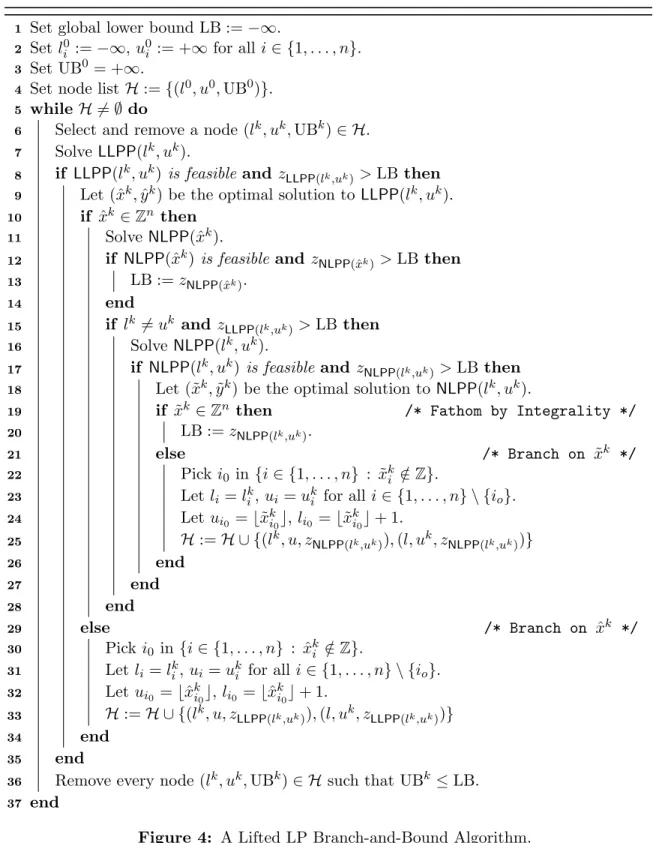
is an upper bound on zNLPP(lk,uk). Furthermore, we denote by LB the global lower bound onzMINLPP and byHthe set of active branch-and-bound nodes. We give in Figure 4 a lifted
LP branch-and-bound algorithm for solvingMINLPP.
A pure NLP based branch-and-bound algorithm solvesNLPP(lk, uk) at each nodekof the
branch-and-bound tree. The idea of the lifted LP branch-and-bound algorithm of Figure 4 is to replace each call to NLPP(lk, uk) in an NLP based branch-and-bound algorithm by a
call toLLPP(lk, uk). After this replacement special care has to be taken when fathoming by
Set global lower bound LB :=−∞. 1 Set l0 i :=−∞,u0i := +∞ for alli∈ {1, . . . , n}. 2 Set UB0 = +∞. 3
Set node listH:={(l0, u0,UB0)}.
4
while H 6=∅do
5
Select and remove a node (lk, uk,UBk)∈ H.
6
SolveLLPP(lk, uk). 7
if LLPP(lk, uk) is feasible and zLLPP(lk,uk)>LBthen
8
Let (ˆxk,yˆk) be the optimal solution toLLPP(lk, uk).
9
if xˆk∈Zn then 10
Solve NLPP(ˆxk). 11
if NLPP(ˆxk) is feasibleand zNLPP(ˆxk)>LBthen
12 LB :=zNLPP(ˆxk). 13 end 14 if lk6=uk and zLLPP(lk,uk)>LBthen 15 Solve NLPP(lk, uk). 16
if NLPP(lk, uk) is feasible and zNLPP(lk,uk)>LB then
17
Let (˜xk,y˜k) be the optimal solution to NLPP(lk, uk).
18
if x˜k∈Zn then /* Fathom by Integrality */ 19 LB :=zNLPP(lk,uk). 20 else /* Branch on x˜k */ 21 Pick i0 in{i∈ {1, . . . , n} : ˜xk i ∈/ Z}. 22 Let li =lk i,ui=uki for all i∈ {1, . . . , n} \ {io}. 23 Let ui0 =bx˜ k i0c,li0 =bx˜ k i0c+ 1. 24 H:=H ∪ {(lk, u, z NLPP(lk,uk)),(l, uk, zNLPP(lk,uk))} 25 end 26 end 27 end 28 else /* Branch on xˆk */ 29 Picki0 in{i∈ {1, . . . , n} : ˆxk i ∈/Z}. 30 Letli =lk i,ui =uki for alli∈ {1, . . . , n} \ {io}. 31 Letui0 =bxˆ k i0c,li0 =bxˆ k i0c+ 1. 32 H:=H ∪ {(lk, u, z LLPP(lk,uk)),(l, uk, zLLPP(lk,uk))} 33 end 34 end 35
Remove every node (lk, uk,UBk)∈ H such that UBk ≤LB.
36
end
37
solution toNLPP(lk, uk). This is handled by the algorithm in lines 11–28. The first step is to
solveNLPP(ˆxk) to attempt to correct an integer feasible solution (ˆxk,yˆk) toLLPP(lk, uk) into
an integer feasible solution to NLPP(lk, uk). If the correction is successful and zNLPP(ˆxk)> LB we can update LB. This step is carried out in lines 11–14 of the algorithm. Another complication arises when the optimal solution toLLPP(lk, uk) is integer feasible, butlk6=uk.
The problem in this case is that integer optimal solutions to LLPP(lk, uk) and NLPP(ˆxk)
may not be solutions to MINLPP(lk, uk). In fact, in this case, it is possible for NLPP(ˆxk)
to be infeasible and for MINLPP(lk, uk) to be feasible. To resolve this issue, the algorithm
of Figure 4 solves NLPP(lk, uk) to process the node in the same way it would be processed
in an NLP based branch-and-bound algorithm forMINLPP. This last step is carried out in
lines 15–28.
Note that, in lines 21–26, the algorithm is effectively branching on a variable xi such that ˆxk
i is integer but for whichlik< uki. Branching on integer feasible variables is sometimes used in MILP (it can be used for example to find alternative optimal solutions) and global optimization (see for example [124]), but to the best of our knowledge it has never been used in the context of polyhedral relaxation based algorithms for convex MINLPs.
We show the correctness of the algorithm in the following proposition.
Proposition 2.1. For any polyhedral relaxationLLPPofNLPP using a bounded polyhedron P, the lifted LP branch-and-bound algorithm of Figure 4 terminates with LB equal to the optimal objective value of MINLPP.
Proof. Finiteness of the algorithm is direct from the fact that P is bounded. However after branching in lines 21–26, solution (ˆxk,yˆk) could be repeated in one of the newly created nodes, which could cause (ˆxk,yˆk) to be generated again in several nodes. This can only happen a finite number of times though, as the branching will eventually causelk =uk or
LLPP(lk, uk) will become infeasible.
All that remains to prove is that the sub-tree rooted at a fathomed node cannot contain an integer feasible solution to MINLPP which has an objective value strictly larger than
17 and 19. In line 8, the node is fathomed if LLPP(lk, uk) is infeasible or if zLLPP(lk,uk) ≤ LB. Because LLPP(lk, uk) is a relaxation of NLPP(lk, uk) we have that infeasibility of LLPP(lk, uk) implies infeasibility of NLPP(lk, uk) and zNLPP(lk,uk)≤zLLPP(lk,uk), hence in both cases we have that the sub-tree rooted at node (lk, uk) cannot contain an integer feasible solution strictly better than the incumbent. In line 15, the node is fathomed if lk = uk or if z
LLPP(lk,uk) ≤ LB. In the first case, NLPP(lk, uk) = NLPP(ˆxk) and hence processing nodekis correctly done by lines 12–14. In the second case, the node is correctly fathomed for the same reasons for correctness in line 8. In line 17, the node is fathomed if
NLPP(lk, uk) is infeasible or if zNLPP(lk,uk) ≤ LB, in either case the sub-tree rooted at the fathomed node cannot contain a integer feasible solution strictly better that the incumbent. Finally, in line 19 the node is fathomed because solution (˜xk,y˜k) toNLPP(lk, uk) is integer feasible and hence it is the best integer feasible solution that can be found at the sub-tree rooted at the fathomed node.
We note that, as in other branch-and-bound algorithms, at any point in the execution of the algorithm we have a lower bound ofzMINLPPgiven by LB and an upper bound given
by max{UBk : (lk, uk,UBk)∈ H}. This can be used for early termination of the algorithm given a target optimality gap.
2.3 Lifted Polyhedral Relaxations
The key idea for the effectiveness of the lifted LP branch-and-bound algorithm is the use of a lifted polyhedral relaxation (q >0) for the construction of LLPP. For the algorithm to
be effective we needNLPP(lk, uk) to be called in as few nodes as possible, so we needLLPP
to be a tight approximation of NLPP. On the other hand we need to solve LLPP(lk, uk)
quickly, which requires the polyhedral relaxation to have relatively few constraints and extra variables. The problem is that using a relaxation with q = 0, such as those constructed using gradient inequalities, can require a polyhedronP with an exponential number of facets to approximate the convex set C tightly. In fact, it is known (see for example [11]) that for any ε > 0 approximating the d-dimensional unit euclidean ball Bd with a polyhedron P ⊂Rd such thatBd⊂ P ⊂(1 +ε)Bdrequires P to have at least exp(d/(2(1 +ε)2)) facets.
However, in many instances, only a few inequalities are needed to optimize over a convex set to a given accuracy. Therefore, current polyhedral relaxation based algorithms do not use a fixed polyhedral relaxation of C and instead dynamically refine the relaxation as needed. On the other hand, when we allow for a polyhedron P in a higher dimensional space we can take advantage of the fact that a lifted polyhedron with a polynomial number of constraints and extra variables can have the same effect as a polyhedron in the original space with an exponential number of facets. Exploiting this property, it is sometimes possible to have a tight lifted polyhedral relaxation ofC that can be described by a reasonable number of inequalities and extra variables. [15] introduced such a lifted polyhedral relaxation for MICP problems. We now give a compact description of the version of the lifted polyhedral relaxation of [15] and [54] we use in this study.
We start by noting that a set CC given by (19) can be written as
CC ={(x, y)∈Rn+p : ∃(z0, z)∈R+×Rr s.t. Ax+By+δ=z,
ax+by+δ0=z0, (z0, z)∈ Lr} whereLr is the (r+ 1)-dimensional Lorentz cone given by
Lr :={(z0, z)∈ R+×Rr : r X k=1 z2 k≤z02}.
Hence a polyhedral relaxation of Lr induces a polyhedral relaxation of CC. Then, for a given tightness parameter ε >0 we want to construct a polyhedron Lr
ε such that Lr
(Lrε({(z0, z)∈R+×Rr : ||z||2 ≤(1 +ε)z0}. (32) To describe this polyhedral relaxation of Lr we assume at first that r = 2p for some p ∈ Z+. We then begin by grouping variables z in Lr into k =r/2 pairs and associate a
new variableρk for thekth pair. We can then rewrite Lr as Lr ={(z0, z)∈ R+×Rr :∃ρ∈Rr/2 s.t. r/2 X k=1 ρ2 k≤z20 z2 2k−1+z2k2 ≤ρ2k fork∈ {1, . . . , r/2}}.
In other words, we can rewriteLrusing (r/2) 3-dimensional Lorentz cones and one (r/2+1)-dimensional Lorentz cone as
Lr={(z0, z)∈
R+×Rr :∃ρ∈Rr/2 s.t.
(ρ, z0)∈ Lr/2
(z2k−1, z2k, ρk)∈ L2 fork∈ {1, . . . , r/2}}.
By recursively applying this procedure to the (r/2 + 1)-dimensional Lorentz cone we can rewrite Lr using only (r−2) 3-dimensional Lorentz cones. We can then replace each of these 3-dimensional Lorentz cones with the polyhedral relaxation of L2 given by
Ws :={(z0, z1, z2)∈R+×R2 : ∃(α, β)∈R2s s.t.
z0 =αscos2πs+βssin2πs α1 =z1cos (π) +z2sin (π) β1 ≥ |z2cos (π)−z1sin (π)| αi+1 =αicosπ
2i
+βisinπ 2i
βi+1 ≥βicos2πi−αisin2πi
fori∈ {1, . . . , s−1}}, for somes∈Z.
For a general r, not necessarily a power of two, these ideas and some careful selection of the parametersinWs yield the polyhedral relaxation ofLr given by
Lr ε:={(z0, z)∈R+×Rr :∃(ζk)Kk=0 ∈RT(r) s.t. z0 =ζK 1 ζ0 i =zi fori∈ {1, . . . , r}, (ζk 2i−1, ζ2i, ζk ik+1)∈ Wsk(ε) fori∈ {1, . . . ,btk/2c}, k∈ {0, . . . , K−1}, ζk tk =ζ k+1 dtk/2e fork∈ {0, . . . , K−1} s.t. tk is odd}
where K = dlog2(r)e, {tk}K
k=0 is defined by the recursion t0 = r, tk+1=dtk/2e for k ∈ {0, . . . , K−1},T(r) =PK k=0tk and sk(ε) = k+ 1 2 − log4 16 9 π−2log(1 +ε) . (33)
From [15] and [54] we have thatLr
εcomplies with (32) for anyε >0 and hasO(nlog(1/ε)) variables and constraints for any 0< ε <1/2.
We can then use Lr
ε to define the relaxation of CC given by
P(CC, ε) ={(x, y)∈Rn+p : ∃(z0, z)∈R+×Rr s.t. Ax+By+δ=z,
ax+by+δ0=z0, (z0, z)∈ Lr
ε}, which complies with
CC ( P(CC, ε) ( {(x, y) ∈ Rn+p : ||Ax +By + δ||2 ≤ (1 + ε)(ax +by + δ0)}. Using this relaxation we can construct the lifted polyhedral relaxation ofCPP given by
zLP(ε):= maxx,y,v cx+dy (34)
s.t.
Dx+Ey≤f (35)
(x, y, v)∈ P(CCi, ε) i∈ I (36)
(x, y, v)∈Rn+p+q (37)
where v ∈ Rq are the auxiliary variables used to construct all P(CCi, ε)’s and P(CCi, ε) is
the polyhedron in Rn+p+q whose projection to Rn+p is P(CCi, ε). We denote the problem
given by (34)–(37) as LP(ε) and the problem given by (34)–(37) and (18) asMILP(ε).
2.4 Computational Results
In this Section we present the results of computational tests showing the effectiveness of the lifted LP branch-and-bound algorithm based onLP(ε). We begin by describing how the
algorithm was implemented, then describe the problem instances we used in the tests and finally we present the computational results.
2.4.1 Implementation
We implemented the lifted LP branch-and-bound algorithm of Figure 4 for LLPP=LP(ε)
and NLPP=CPP by modifying CPLEX 10.0’s MILP solver. We used the branch callback
feature to implement branching on integer feasible solutions when necessary and we used the incumbent and heuristic callback features to implement the solve of NLPP(ˆxk). All
coding was done in C++ using Ilog Concert Technology. We used CPLEX’s barrier solver to solveCPP(lk, uk) andCPP(ˆx). In all cases we used CPLEX’s default settings. We denote
this implementation as LP(ε) -BB .
There are some technical differences between this implementation and the lifted LP branch-and-bound algorithm of Figure 4. First, in the CPLEX based implementation,
NLPP(ˆxk) is solved for all integer feasible solutions found. This is a difference because
the algorithm of Figure 4 only finds integer solutions when LLPP(lk, uk) is integer
feasi-ble, but CPLEX also finds integer feasible solutions by using primal heuristics. Finally, the implementation benefits from other advanced CPLEX features such as preprocessing, cutting planes and sophisticated branching and node selection schemes. In particular, the addition of cutting planes conceptually modifies the algorithm as adding these cuts updates the polyhedral relaxation definingLLPP. This updating does not use any information from
the nonlinear constraints though, as CPLEX’s cutting planes are only derived using the linear constraints of LLPPand the integrality of thex variables.
2.4.2 Test Instances
Our test set consists of three different portfolio optimization problems with cardinality constraints from the literature [31, 86, 85]. For most portfolio optimization problems only the continuous variables are present in the nonlinear constraints and hence the convex hull of integer feasible solutions to these problems is almost never a polyhedron. Furthermore, polyhedral relaxation based algorithms for the purely continuous versions of these problems are known to converge slowly. For these reasons we believe that portfolio optimization problems are a good set of problems to test the effectiveness of the lifted LP branch-and-bound algorithm based onLP(ε).
For all three problems we let ai be the random return on stock iand let the expected value and covariance matrix of the joint distribution of a= (a1, . . . , an) be ¯a∈Rn+ and Q respectively. Also, letyi be the fraction of the portfolio invested in stockiandQ1/2 be the positive semidefinite square root of Q.
The first problem is obtained by adding a cardinality constraint to the classical mean-variance portfolio optimization model to obtain the MICP problem already explained in (20)–(26). We refer to the set of instances of this problem as theclassical instances.
The second problem is constructed by replacing the variance risk constraint (21) of the classical mean-variance model with two shortfall risk constraints of the form Prob(¯ay≥Wlow)≥η. Following [86] and [85] we formulate this model as a conic quadratic programming problem obtained by replacing constraint (21) in the classical mean-variance problem with
Φ−1(ηi)||Q1/2y||
2 ≤¯ay−Wilow i∈ {1,2}
where Φ(·) is the cumulative distribution function of a zero mean, unit variance Gaussian random variable. We refer to the set of instances of this problem as theshortfall instances. The final problem is a robust portfolio optimization problem studied in [31]. This model assumes that there is some uncertainty in the expected returns ¯a and that the true expected return vector is normally distributed with mean ¯aand covariance matrixR. The model is similar to one introduced in [13] and can be formulated as the conic quadratic programming problem obtained by replacing the objective function (20) of the classical mean-variance with maxx,y,rr and adding the constraint ¯ay−α||R1/2y||2 ≥r whereR1/2 is the positive semidefinite square root ofR. The effect of this change is the maximization of ¯
ay−α||R1/2y||
2 which is a robust version of the maximization of the expected return ¯ay. We refer to the set of instances of this problem as therobust instances.
We generated the data for the classical instances in a manner similar to the test instances of [85]. We first estimated ¯aand Qfrom 251 daily closing prices of S&P 500 stocks starting with the 22nd of August 2005 and we scaled the distributions for a portfolio holding period of 20 days. Then, for each n we generated an instance by randomly selecting nstocks out of the 462 stocks for which we had closing price data. We also arbitrarily selected σ = 0.2
and K= 10.
For the shortfall instances we used the same data generated for the classical mean-variance instances, but we additionally included a risk-less asset with unit return to make these instances differ even more from the classical mean-variance instances. Also, in a manner similar to the test sets of [85] we arbitrarily selected η1 = 80%, Wlow
1 = 0.9, η2 = 97%,Wlow
2 = 0.7.
Finally, we generated the data for the robust instances in a manner similar to the test instances of [31]. We used the same daily closing prices used for the classical mean-variance and shortfall risk constraints instances, but we randomly selected different groups ofnstocks and we generated the data in a slightly different way. For stock iwe begin by calculating µi as the mean daily return from the first 120 days available. We then let ¯ai= 0.1µi+ 0.9r whereris the daily return for the 121st day. FinallyQis estimated from the same first 120 days and following [31] we let R = (0.9/120)Q. We also arbitrarily selected α = 3 and we again selected σ= 0.2 and K= 10.
For the three sets of instances we generated 100 instances for each n in{20,30,40,50} and 10 instanced for each n in {100,200}. All data sets are available at http://www2. isye.gatech.edu/~jvielma/portfolio.
2.4.3 Results
All computational tests where done on a dual 2.4GHz Xeon workstation with 2GB of RAM running Linux Kernel 2.4. The first set of experiments show calibration results for different values of ε. We then study how LP(ε) -BB compares to other algorithms. Finally, we
study some factors that might affect the effectiveness ofLP(ε).
2.4.3.1 Selection of ε
Note that as εgets smaller the size of LP(ε) grows asO(nlog(1/ε)), on the other hand the
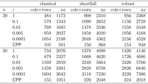
relaxation gets tighter. To select the value ofεfor subsequent runs we first studied the sizes ofLP(ε) fornin{20,30}and for values ofεin{1,0.1,0.01,0.001,0.0001}. Table 1 presents
Table 1: Problem Sizes for Different Values ofε
classical shortfall robust
n ε cols+rows nz cols+rows nz cols+rows nz
20 1 484 1172 908 2310 956 2368 0.1 579 1343 1098 2652 1156 2728 0.01 769 1685 1478 3336 1556 3448 0.001 959 2027 1858 4020 1956 4168 0.0001 1054 2198 2048 4362 2156 4528 CPP 105 501 150 968 154 948 30 1 734 2076 1378 4098 1426 4146 0.1 879 2337 1668 4620 1726 4686 0.01 1169 2859 2248 5664 2326 5766 0.001 1459 3381 2828 6708 2926 6846 0.0001 1604 3642 3118 7230 3226 7386 CPP 155 1051 220 2048 224 2018
The table also includes the same information forCPP.
We see that the sizes of LP(ε) are considerable larger that the sizes of CPP. On the
other hand we confirm that sizes only grow logarithmically with ε.
We additionally devised the following simple computational experiment for selecting the appropriate value of ε. Forn equal to 20 and 30 we selected the first 10 instances of each instance class and tried to solve them with values ofεin{1,0.1,0.01,0.001,0.0001}. A time limit of 100 seconds was set. Note that, although Proposition 2.1 shows that LP(ε) -BB
solves the problem exactly (up to the precision of the continuous relaxation solvers) for any ε, for efficiency reasons we would probably never select ε = 1 as the resulting relaxation is too weak. However, we decided to test it anyway to illustrate that the procedure works even for this extreme choice of ε.
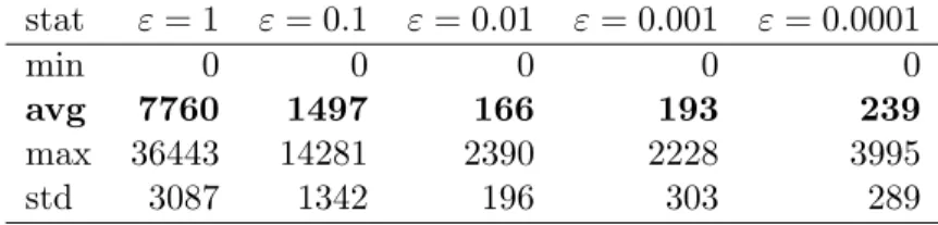
Table 2 shows the minimum, average, maximum and standard deviation of the number of nodes needed by LP(ε) -BB to solve the instances. Tables 3 and 4 show the same
statistics for solve times in seconds and the number of branch-and-bound nodes in which nonlinear relaxation CPP(lk, uk) is solved.
Table 2: Number of Nodes for Different Values of ε stat ε= 1 ε= 0.1 ε= 0.01 ε= 0.001 ε= 0.0001 min 0 0 0 0 0 avg 7760 1497 166 193 239 max 36443 14281 2390 2228 3995 std 3087 1342 196 303 289
Table 3: Solve Time for Different Values ofε[s] stat ε= 1 ε= 0.1 ε= 0.01 ε= 0.001 ε= 0.0001
min 0.14 0.07 0.09 0.12 0.18
avg 37.18 3.71 1.10 3.19 5.79
max 100.31 21.28 8.64 35.38 71.16
std 21.61 3.33 1.16 5.53 10.53
Table 4: Number of Nodes that SolveCPP(lk, uk)
stat ε= 1 ε= 0.1 ε= 0.01 ε= 0.001 ε= 0.0001
min 1 1 1 0 0
avg 1700 74 4 3 3
max 6178 367 18 22 23
std 436 25 2 3 1
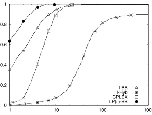
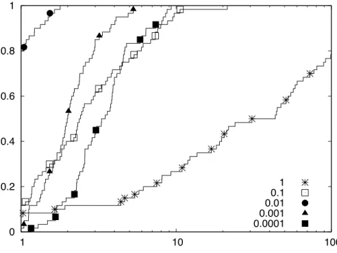
a performance metric. For a given valuem on the horizontal axis and a given method, the valuef plotted in the performance profile indicates the fractionf of the instances that were solved by that method withinmtimes the length of time required by the fastest method for each instance. In particular, the intercepts of the plot (if any) with the vertical axis to the left and right indicate the fraction of the instances for which the method was the fastest and the fraction of the instances which the method could solve in the alloted time, respectively. For example, the method forε= 1 was the fastest in about 5% of the instances, could solve almost 80% of the instances and could solve under 30% of the instances within 10 times the length of time required by the fastest solver. Note that these profiles are step functions. In Figure 5, and all subsequent performance figures, we mark a small subset of the data points to distinguish the individual profiles. We refer the reader to [48] for more details about the construction and interpretation of performance profiles.
0 0.2 0.4 0.6 0.8 1 1 10 100 1 0.1 0.01 0.001 0.0001
Figure 5: Performance Profile for Different Values of ε
We see that ε = 0.01 is the best choice on average. It also has the best performance profile and it yields the fastest method for 80% of the instances. Furthermore, forε= 0.01 we have very few nodes solvingCPP(lk, uk).
It is also interesting to note that the procedure still works fairly well for values of εas big as 0.1 and even for the extreme case ofε= 1 the procedure was still able to solve almost 80% of the instances in the alloted time of 100 seconds. For this last case though, the high number of nodes that solve CPP(lk, uk) makes the algorithm behave almost like an NLP
based branch-and-bound algorithm.
Finally, we note that the result that ε= 0.01 requires the smallest number of branch-and-bound nodes on average is somewhat unexpected. This contradicts the belief that the algorithm of Figure 4 should require fewer branch-and-bound nodes if tighter relaxations are used. An explanation of this apparent contradiction comes from the difference between the algorithm of Figure 4 and the implementation of LP(ε) -BB as discussed in Section
2.4.1, since the use of CPLEX’s advanced features in LP(ε) -BB makes it hard to predict
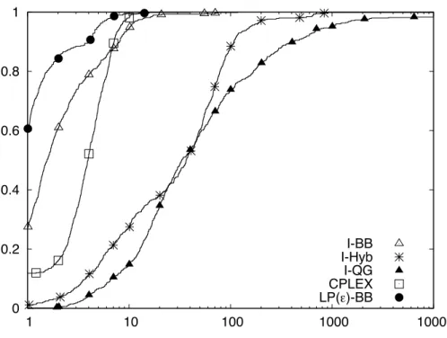
0 0.2 0.4 0.6 0.8 1 1 10 100 1000 10000 I-BB I-Hyb I-QG CPLEX LP(!)-BB
Figure 6: Performance Profile for Small Instances
2.4.3.2 Performance of LP(ε)-BB against other methods
In this Section we compare LP(ε) -BB with ε = 0.01 against other solvers. The solvers
we choose for the comparison are the NLP based branch-and-bound algorithms CPLEX 10 MICP solver and Bonmin’s I-BB and the polyhedral relaxation based algorithms I-QG and I-Hyb from Bonmin. We did not include Bonmin’s I-OA algorithm as it performed very badly in preliminary tests.
For CPLEX we used its default settings and for the Bonmin solvers we set parameters allowable gap and allowable fraction gap to 10−6 and 10−4 respectively to have the same target gaps as CPLEX. All tests were run with a time limit of 10000 seconds.
We first tested all solvers for all instances for n in {20,30}. We denote this set of instances as the small instances. Table 5 shows the minimum, average, maximum and standard deviations of the solve times. Figure 6 shows the performance profile for all the instances using solve time as a performance metric.
Table 5: Solve Times for Small Instances [s]
instance(n) stat LP(ε) -BB I-QG I-Hyb I-BB CPLEX
classical(20) min 0.08 0.38 0.22 0.28 0.02 avg 0.29 26.41 24.84 1.28 1.31 max 1.06 222.19 164.71 13.33 7.95 std 0.18 42.92 26.37 2.31 1.17 classical(30) min 0.25 1.62 0.33 0.38 0.73 avg 1.65 1434.86 217.25 13.19 9.68 max 27.0 10005.2 10003.3 573.97 324.63 std 3.21 2768.34 1016.68 59.17 33.68 shortfall(20) min 0.19 0.18 0.26 0.34 0.03 avg 0.48 17.42 16.78 0.63 1.68 max 1.65 174.62 58.45 3.52 5.19 std 0.21 30.77 17.96 0.52 0.89 shortfall(30) min 0.4 1.25 0.57 0.47 1.26 avg 2.20 847.63 136.39 5.00 9.26 max 29.34 10003.1 5907.32 73.81 80.36 std 3.21 1992.86 588.61 10.00 12.20 robust(20) min 0.19 0.39 0.12 0.37 0.03 avg 0.39 4.99 15.51 2.57 1.03 max 1.05 33.85 599.46 57.22 3.5 std 0.20 5.60 60.37 10.25 0.90 robust(30) min 0.43 0.59 0.29 0.48 0.07 avg 1.20 75.07 23.43 1.02 3.54 max 4.72 2071.47 134.08 4.92 10.76 std 0.81 284.39 25.49 0.87 2.45
set of instances and that this average can be up to five times better than the average for its closest competitor. Furthermore, as the standard deviation and maximum numbers show,
LP(ε) -BB is far more consistent in providing good solve times than the other methods.
From Figure 6 we can also see that LP(ε) -BB has the best performance profile, that it is
the fastest solver in 60% of the instances and that it is almost never an order of magnitude slower than the best solver.
Our second set of tests include all instances for n in {40,50}. We denote this set of instances as themedium instances. We did not include I-QG in these tests as it performed very poorly on the instances for n = 30 and reached the time limit in several instances. Although I-Hyb performed close to I-QC we included it in these tests as it had only reached the time limit in one instance and we wanted to have at least one of the original LP/NLP
based branch-and-bound solvers in our tests. Table 6 shows the minimum, average, maxi-mum and standard deviation of the solve times. Figure 7 shows the performance profile for all the instances using solve time as a performance metric.
Table 6: Solve Times for Medium Instances [s]
instance(n) stat LP(ε) -BB I-Hyb I-BB CPLEX
classical(40) min 0.56 35.04 0.61 1.55 avg 14.84 1412.23 144.17 63.41 max 554.52 10006.0 8518.95 2033.65 std 56.64 2631.92 848.84 208.86 classical(50) min 0.76 35.17 0.75 4.12 avg 102.88 4139.92 894.00 636.83 max 1950.81 12577.8 10030.1 10000.0 std 270.96 4343.71 2048.96 1626.37 shortfall(40) min 1.17 34.72 0.7 4.93 avg 16.60 956.98 92.85 111.97 max 389.57 10004.6 4888.26 4259.5 std 43.85 2133.56 489.98 430.95 shortfall(50) min 1.58 33.22 0.96 5.69 avg 163.10 3143.84 452.05 567.74 max 7674.86 10006.0 10034.1 10000.0 std 771.98 3803.14 1285.52 1319.39 robust(40) min 0.51 0.43 0.69 0.14 avg 3.82 59.10 4.31 11.17 max 42.57 1141.91 129.82 160.71 std 6.04 130.37 14.64 18.58 robust(50) min 0.92 0.65 0.93 0.25 avg 20.44 435.43 23.67 41.71 max 443.29 10002.1 746.37 876.31 std 63.47 1702.15 95.68 120.24
We see from Table 6 that LP(ε) -BB is now the fastest algorithm on average for all
instances and this average can be up to six times better than the average for its closest competitor. Again, as the standard deviation and maximum numbers show, LP(ε) -BB is
far more consistent in providing good solve times than the other methods. From Figure 7 we again see that LP(ε) -BB has the best performance profile, that it is the fastest solver
in over 60% of the instances and that it is almost never an order of magnitude slower than the best solver. Moreover, it is the only solver with this last property.
0 0.2 0.4 0.6 0.8 1 1 10 100 1000 I-BB I-Hyb CPLEX LP(!)-BB
Figure 7: Performance Profile for Medium Instances
Our last set of tests include instances fornin{100,200}. We denote this set of instances as the large instances. We do not include the results for I-Hyb as it was not able to solve any of the instances in this group. Neither did we include results for the classical or shortfall instances for n = 200 as none of the methods could solve a single instance in the alloted time. Table 7 shows the minimum, average and maximum of the solve times. We did not include standard deviations as time limits were reached for too many instances. We instead include the number of instances (out of a total of 10 per instance class) that each method could solve in the alloted time. Figure 8 shows the performance profile for all the instances using solve time as a performance metric.
From Table 7 we see that LP(ε) -BB is the fastest algorithm on average for all but one
set of instances in this group. Furthermore, for all instance classes it is the method that solves the largest number of instances. From Figure 8 we can also see that LP(ε) -BB has
the best performance profile, that it is the fastest solver in about 40% of the instances and that it is the method that is able to solve the greatest number of instances in the alloted
![Table 5: Solve Times for Small Instances [s]](https://thumb-us.123doks.com/thumbv2/123dok_us/10219446.2925807/44.918.217.754.159.675/table-solve-times-for-small-instances-s.webp)
![Table 6: Solve Times for Medium Instances [s]](https://thumb-us.123doks.com/thumbv2/123dok_us/10219446.2925807/45.918.248.723.294.813/table-solve-times-for-medium-instances-s.webp)