Stochastic dynamic programming with factored representations

Stochastic dynamic programming with factored

representations

Craig Boutilier

, Richard Dearden

, Moisés Goldszmidt

c_{Computer Science Department, Stanford University, Stanford, CA 94305-9010, USA} Received 16 July 1999

Abstract

Markov decision processes (MDPs) have proven to be popular models for decision-theoretic planning, but standard dynamic programming algorithms for solving MDPs rely on explicit, state-based specifications and computations. To alleviate the combinatorial problems associated with such methods, we propose new representational and computational techniques for MDPs that exploit certain types of problem structure. We use dynamic Bayesian networks (with decision trees representing the local families of conditional probability distributions) to represent stochastic actions in an MDP, together with a decision-tree representation of rewards. Based on this representation, we develop versions of standard dynamic programming algorithms that directly manipulate decision-tree representations of policies and value functions. This generally obviates the need for state-by-state computation, aggregating state-by-states at the leaves of these trees and requiring computations only for each aggregate state. The key to these algorithms is a decision-theoretic generalization of classic regression analysis, in which we determine the features relevant to predicting expected value. We demonstrate the method empirically on several planning problems, showing significant savings for certain types of domains. We also identify certain classes of problems for which this technique fails to perform well and suggest extensions and related ideas that may prove useful in such circumstances. We also briefly describe an approximation scheme based on this approach.2000 Elsevier Science B.V. All rights reserved.

✩

Some parts of this report appeared in preliminary form in “Exploiting Structure in Policy Construction”, in: Proc. Fourteenth International Joint Conference on Artificial Intelligence (IJCAI-95), Montreal, Quebec, pp. 1550–1556 (1995); and in “Correlated Action Effects in Decision-Theoretic Regression”, in: Proc. Thirteenth

Conference on Uncertainty in Artificial Intelligence (UAI-97), Providence, RI, pp. 30–37 (1997).

∗_{Corresponding author.}

E-mail addresses: [email protected] (C. Boutilier), [email protected] (R. Dearden),

[email protected] (M. Goldszmidt).

0004-3702/00/$ – see front matter 2000 Elsevier Science B.V. All rights reserved. PII: S 0 0 0 4 - 3 7 0 2 ( 0 0 ) 0 0 0 3 3 - 3

Keywords: Decision-theoretic planning; Markov decision processes; Bayesian networks; Regression; Decision

trees; Abstraction

1. Introduction

Decision-theoretic planning (DTP) has attracted a considerable amount of attention recently as AI researchers seek to generalize the types of planning problems that can be tackled in computationally effective ways. DTP is primarily concerned with problems of sequential decision making under conditions of uncertainty and where there exist multiple, often conflicting, objectives whose desirability can be quantified. Markov

decision processes (MDPs) have been adopted as the model of choice for DTP problems in

much recent work [12,26,28,30,61,78], and have also provided the underlying foundations for most work in reinforcement learning [48,76,77,84]. MDPs allow the introduction of uncertainty into the effects of actions, the modeling of uncertain exogenous events, the presence of multiple, prioritized objectives, and the solution of nonterminating process-oriented problems.1

The foundations and the basic computational techniques for MDPs [3,5,44,62] are well-understood and in certain cases can be used directly in DTP. These methods exploit the dynamic programming principle and allow MDPs to be solved in time polynomial in the size of the state and action spaces that make up the planning problem. Unfortunately, these classical dynamic programming methods are formulated so as to require explicit state space enumeration. As such, AI planning systems that solve MDPs are faced with Bellman’s so-called curse of dimensionality: the number of states grows exponentially with the number of variables that characterize the planning domain. This has an impact on the feasibility of both the specification and solution of large MDPs.

The curse of dimensionality plagues not only DTP, but also classical planning techniques. However, methods have been developed that, in many instances, circumvent this problem. In classical planning one typically does not specify actions and goals explicitly using the underlying state space, but rather “intensionally” using propositional or variable-based representations. For instance, a STRIPS representation of an action describes very concisely the transitions induced by that action over a large number of states. Similarly, classical planning techniques such as regression planning [83] or nonlinear planning [22,54,58,66] exploit these representations to great effect, never requiring that one search (or implement “shortest-path” dynamic programming techniques) explicitly through state space. Intuitively, such methods aggregate states that behave identically under a given action sequence with respect to a given goal.

In this paper, we develop similar techniques for solving certain classes of large MDPs. We first describe a representation for actions with stochastic effects that uses Bayesian networks (and decision trees to represent the required families of conditional probability 1_{One form of uncertainty cannot be handled in the framework we adopt, specifically, partial observability, or} uncertain knowledge about the state of the system being controlled. Partially observable MDPs (or POMDPs) [52,53,73,75] can be used in such cases. We will make further remarks on POMDPs at the end of this article.

distributions) to provide the same type of compact representation of actions that, say, STRIPS affords in deterministic settings. We also use decision trees to represent reward functions. This representation lays bare—indeed, exploits—certain structural regularities in transition probabilities and reward functions. We then describe algorithms that use this representation to compute value functions and solve MDPs without generally requiring explicit enumeration of the state space. Much like regression in classical planning, we focus attention on the variables that, under a particular action, influence the outcome of this action with respect to relevant variables. In addition, policies and value functions will be represented compactly using decision trees, with the structure inherent in the policy or value function being preserved to a large extent by our algorithmic operations. Indeed, under certain assumptions one can show that the degree of preserved structure is maximal (e.g., subject to variable reordering in trees).

1.1. Decision-theoretic regression

The key to each of our algorithms is a process we call decision-theoretic regression. In classical planning the regression of a set of conditionsCthrough an actionais the weakest set of conditions regr(C, a) such that performing action a under conditions regr(C, a) ensures thatCis made true [83].2 This is the key step in any backchaining (or subgoaling) planner, including least-commitment planners [54,58]. Given a (sub)goal setG, regression ofGthrougha produces a new subgoal whose achievement with planP0 assures us of a planP to achieveG: simply appendatoP0to formP.

Decision-theoretic regression generalizes this process in two ways. First, we cannot always speak of goal achievement in MDPs; rather, we concern ourselves with the value associated with certain conditions. Thus, we regress a set of conditions, each associated with a distinct value, through an action. As such, the decision-theoretic regression of such a set of conditions through an action will result in a new set of conditions. Second, stochastic actions rarely guarantee achievement of any particular condition—so rather than producing the conditions that, when the action is applied, lead to a specific “target” condition, we instead produce a set of conditions under which the action will make each of the regressed conditions true with identical probability. It follows that, since each condition in the regressed set is associated with a single value, the new conditions produced by decision-theoretic regression each have the same expected value under actiona.

With such an operation in hand, we can implement classical algorithms for solving MDPs, such as value iteration [3] or modified policy iteration [63] in a highly structured way. Our structured versions of these algorithms will cluster together states that at each stage in the computation have the same estimated value or same optimal choice of action. This partitioning of state space into such regions will be represented by decision trees that test the values of specific variables. The computational advantage provided by such an approach is that value need only be computed once for each region instead of once per state.

1.2. State aggregation and function approximation

The approach we take to solving large MDPs is a specific state aggregation method. Other types of state aggregation techniques have been proposed, in which states with similar characteristics are grouped together. Such methods are reported in, for instance, [4,68,81], and can vary as to whether states are statically or dynamically aggregated (that is, do the groupings of states stay fixed or can they change during computation). Other compact representations of value functions have also been proposed, such as linear function representations or neural networks [1,6,80,81]. These techniques do not seek to exploit regions of uniformity in value functions, but rather compact functions of state features that reflect value. As such they are distinguished from strict aggregation methods.

In much of this previous work, the goal is the approximate solution of large MDPs. Our proposal can be distinguished from other aggregation methods, and other compact representations of values functions, in two major ways. First, our aggregations are determined dynamically using features that are easily extracted from the model. In this sense, the intuitions that underly our approach are much more closely aligned with those exploited in classical planning. Indeed, states are implicitly aggregated by a process of

abstraction—the removing of certain variables from the state space description. Second,

our methods are not (inherently) approximation techniques—the basic procedures produce exact solutions and value functions.3 We will, however, describe modifications of our techniques that allow approximate solutions to be constructed.

There are two approaches to state aggregation that bear similarity to our method. The first is the model minimization approach of Givan and Dean [26,27,39]. In this work, the notion of automaton minimization [42,51] is extended to MDPs and is used to analyze abstraction techniques such as those presented in [30]. More closely related to the specific model we propose in the current paper is that of Dietterich and Flann [32,33]. They apply regression methods to the solution of MDPs (and consider this problem in the context of reinforcement learning in addition). Their original proposal [32] is restricted to MDPs with goal regions and deterministic actions (represented using STRIPS operators), thus rendering true goal-regression techniques directly applicable. This is extended in [33] to allow stochastic actions, thus providing a stochastic generalization of goal regression. We discuss these models in more detail in Section 4.7.

1.3. Outline

In Section 2 we describe the basic MDP model, various concepts that are used in the solution of MDPs, as well as several classical algorithms for solving MDPs.

In Section 3, we define a particular compact representation of an MDP, using dynamic

Bayesian networks [25,29]—a special form of Bayesian network [57]—to represent the

dependence between variables before and after the occurrence of actions. In addition, we use decision trees to represent the conditional probability matrices quantifying the 3_{More accurately, they produce solutions that are identical to their standard state-based counterparts, which} may beε-optimal.

network to exploit context-specific independence [14], that is, independence given a particular variable assignment. We note that this representation is somewhat related to the probabilistic variants of STRIPS operators introduced in [40] and augmented in [30]. We also describe the decision-tree representation of reward functions, value functions and policies.

In Section 4, we describe the basic decision-theoretic regression operator which, given a particular tree-structured value function and action network, regresses the value function through that action to produce a new value function. With this operation in hand, we develop structured analogs of classical MDP algorithms like value and policy iteration. In Section 5 we present an empirical analysis of these methods and suggest the types of problems for which it is likely to work well, unlikely to work well, and what possible approaches may help with the latter. In Section 6 we describe an extension of the algorithms presented in Section 4 to deal with correlations in action effects. We also briefly describe some work that leverages the structured methods described in Section 4 to provide

approximate solutions for structured MDPs. We conclude in Section 7 with some brief

discussion of recent work that is related to, or extends, these ideas, and describe some promising directions for future research.

2. Markov decision processes

MDPs can be viewed as stochastic automata in which actions have uncertain effects, inducing stochastic transitions between states, and in which the precise state of the system is known only with a certain probability. In addition, the expected value of a certain course of action is a function of the transitions it induces, allowing rewards to be associated with different aspects of the problem rather than with an all-or-nothing goal proposition. Finally, plans can be optimized over a fixed finite period of time, or over an infinite horizon, the latter suitable for modeling ongoing processes. These make MDPs ideal models for many decision-theoretic planning problems (for further discussion of the desirable features of MDPs from the perspective of modeling DTP problems, see [11,17,28,35]).

In this section, we describe the basic MDP model and consider several classical solution procedures. Primarily for reasons of presentation, we do not consider action costs in our formulation of MDPs. All utilities are associated with states (or propositions). However, more general cost/reward models could easily be incorporated with our framework. Furthermore, we restrict our attention to finite state and action spaces. Finally, we make the assumption of full observability: despite the uncertainty associated with action effects, the planning (or plan-executing) agent can observe the exact outcome of any action it has taken and knows the precise state of the system at any time. Partially observable MDPs (POMDPs) [21,53,73] are much more computationally demanding than fully observable MDPs. However, we will make a few remarks on the application of our techniques to POMDPs at the conclusion of this article.4

We refer the reader to [5,11,62] for further material on MDPs. 4_{See [16] for more detailed investigations of this type.}

2.1. The basic model

A Markov decision process can be defined as a tuplehS,A, T , Ri, whereSis a finite set of states or possible worlds,Ais a finite set of actions,T is a state transition function, and R is a reward function. A state is a description of the system of interest that captures all information about the system relevant to the problem at hand. In typical planning applications, the state is a possible world, or truth assignment to the logical propositions with which the system is described. The agent can control the state of the system to some extent by performing actionsa∈Athat cause state transitions, movement from the current state to some new state. Actions are stochastic in that the actual transition caused cannot generally be predicted with certainty. The transition function T describes the effects of each action at each state.T (si, a)is a probability distribution overS:T (si, a)(sj)is the

probability of ending up in statesj ∈S when actiona is performed at statesj. We will

denote this quantity by Pr(si, a, sj). We require that 06Pr(si, a, sj)61 for all si, sj,

and that for all si,P_sj∈SPr(si, a, sj)=1. The componentsS,A andT determine the

dynamics of the system being controlled. We assume that each action can be performed at each state. In more general models, each state can have a different feasible action set, but this is not crucial here.5

The states that the system passes through as actions are performed correspond to the

stages of the process. The system starts in a statesiat stage 0. Aftertactions are performed,

the system is at staget. Given a fixed “course of action,” the state of the system at staget can be viewed as a random variableSt; similarly, we denote byAt the action executed at staget. Stages provide a rough notion of time for MDPs. The system is Markovian due to the nature of the transition function; that is,

Pr St|At−1, St−1, At−2, St−2, . . . , A0, S0=Pr St|At−1, St−1.

The fact that the system is fully observable means that the agent knows the true state at each stage t (once that stage is reached), and its decisions can be based solely on this knowledge.

A stationary, Markovian policyπ:S→Adescribes a course of action to be adopted by an agent controlling the system and plays the same role as a plan in classical planning. An agent adopting such a policy performs actionπ(s)whenever it finds itself in state s. Such policies are Markovian in the sense that action choice at any state does not depend on the previous system history, and are stationary since action choice does not depend on the stage of the decision problem. For the problems we consider, optimal stationary, Markovian policies always exist. In a sense, π is a conditional and universal plan [67], specifying an action to perform in every possible circumstance. An agent following policy π can also be thought of as a reactive system.

A number of optimality criteria can be adopted to measure the value of a policy π. We assume a bounded, real-valued reward functionR:S→R.R(s)is the instantaneous 5_{We could model the applicability conditions for actions using preconditions in a way that fits within our} framework below. However, we prefer to think of actions as action attempts, which the agent can execute (possibly without effect or success) at any state. Preconditions may be useful to restrict the planning agent’s attention to potentially “useful” actions, and thus can be viewed as a form of heuristic guidance (e.g., do not bother considering attempting to open a locked door). This will not impact what follows in any important ways.

reward an agent receives for occupying states. More general reward models are possible, though none of these introduce any special complications for our algorithms. One common generalization allows R(s) to be a random variable—if this is the case, taking its expectation as the (deterministic) reward for state s has no impact on value or policy calculations.6 Often one allows reward R(s, a)to depend on the action taken, so as to model the costs of various actions. To keep the presentation simple, we will not consider this possibility in the development of our algorithms; but we will point out the very minor adjustments one must make to account for action costs at appropriate points in the presentation of our methods.

We take a Markov decision problem to be an MDP together with a specific optimality criterion. We will use the abbreviation MDP to refer to the specific problem (process with optimality criterion) as well as the process, with context distinguishing the precise meaning. Optimality criteria vary with the horizon of the process being controlled and the manner in which future reward is valued. In this paper, we focus on discounted

infinite-horizon problems: the current value of a reward receivedtstages in the future is discounted by some factorβt_{(06β <1). This allows simpler computational methods to be used, as}

discounted total reward will be finite.7 The infinite-horizon model is important because, even if a planning problem does not proceed for an infinite number of stages, the horizon is usually indefinite, and can only be bounded loosely. Furthermore, solving an inhorizon problem is often more computationally tractable than solving a very long finite-horizon problem. Discounting has certain other attractive features, such as encouraging plans that achieve goals quickly, and can sometimes be motivated on economic grounds, or can be justified as modeling expected total reward in a setting where the process has probability 1−β of terminating (e.g., the agent breaks down) at each stage. We refer to [62] for further discussion of MDPs and different optimality criteria.

The value of a policyπ (under this optimality criterion) is simply the expected sum of discounted future rewards obtained by executingπ. Since this value depends on the state in which the process begins, we useVπ(s)to denote the value ofπ at states. A policyπ∗is

optimal if, for alls∈Sand all policiesπ, we haveVπ∗(s)>Vπ(s). We are guaranteed that

such optimal (stationary) policies exist in our setting [62]. The (optimal) value of a state V∗(s)is its valueVπ∗(s)under any optimal policyπ∗. We take the problem of

decision-theoretic planning to be that of determining an optimal policy (or an approximately optimal or satisficing policy).

2.2. Solution methods

Policy evaluation and successive approximation

Given a fixed policy π, the function Vπ can be computed using a straightforward

iterative algorithm know as successive approximation [5,62]. We proceed by constructing a sequence of n-stage-to-go value functionsV_πn. The quantityV_πn(si)is the expected sum

6_{Similarly, if rewards depend on the transition froms}

itosj (i.e., take the formR(si, sj)) expectations can be

used if we allow reward to depend on actions, as we discuss below.

7_{Our methods apply directly to finite-horizon problems as well, and with suitable modification can be used in} the computation of average-optimal policies. We do not pursue this here.

of discounted future rewards received whenπ is executed fornstages starting at statesi.

We setV_π0(si)=R(si)and recursively compute

V_πn(si)=R(si)+β X sj∈S Pr si, π(si), sj V_πn−1(sj). (1)

Asn→ ∞,V_πn→Vπ; and the convergence rate and error for a fixedncan be bounded

[62]. We note that the right-hand side of this equation determines a contraction operator so that: (a) the algorithm converges for any starting estimateV_π0; and (b) if we setV_π0=Vπ,

then the computedV_πnfor anynis equal toVπ (i.e.,Vπ is a fixed-point of this operator).

We can also compute the value functionVπ exactly using the following formula due to

Howard [44]: Vπ(si)=R(si)+β X sj∈S Pr si, π(si), sj Vπ(sj). (2)

We can find the value ofπfor all states by solving this set of linear equationsVπ(s), ∀s∈ S.

Value iteration

By solving an MDP, we refer to the problem of constructing an optimal policy. Value

iteration [3] is a simple iterative approximation algorithm for optimal policy construction

that proceeds much like successive approximation, except that at each stage we choose the action that maximizes the right-hand side of Eq. (1):

Vn(si)=R(si)+max a∈A β X sj∈S Pr(si, a, sj)Vn−1(sj) . (3)

The computation ofVn_(s)givenVn−1 _{is known as a Bellman backup. The sequence of} value functionsVn _{produced by value iteration converges linearly toV}∗_{. Each iteration}

of value iteration requires O(|S|2_{|A|)computation time, and the number of iterations is} polynomial in|S|.

For some finiten, the actionsa that maximize the right-hand side of Eq. (3) form an optimal policy, andVn_{approximates its value.}

One simple stopping criterion requires termination when Vi+1−Vi6ε(1−β)

2β (4)

(wherekXk =max{|x|: x∈X}denotes the supremum norm). This ensures the resulting value function Vi+1is within ε/2 of the optimal function V∗ at any state, and that the induced policy is ε-optimal (i.e., its value is within ε of V∗) [62]. Another stopping criterion uses the span seminorm, kVi+1 −Viks, where kXks =max{x: x ∈X} −

min{x:x∈X}. Similar bounds on the quality of the induced policy can be provided.8 8_{We refer to [62] for a detailed discussion of more refined stopping criteria and error bounds for value} iteration, and how assurances of optimality (rather thanε-optimality) can be provided using techniques like action elimination.

A concept that will be useful later is that of a Q-function. Given an arbitrary value functionV, we defineQV_a(s)as QV_a(si)=R(si)+β X sj∈S Pr(si, a, sj)V (sj). (5)

Intuitively,QV_a(s)denotes the value of performing actionaat statesand then acting in a manner that has valueV [84]. In particular, we defineQ∗_ato be the Q-function defined with respect toV∗, andQn_ato be the Q-function defined with respect toVn−1. In this manner, we can rewrite Eq. (3) as:

Vn(s)=max

a∈A

Qn_a(s) . (6)

Policy iteration

Policy iteration [44] is another optimal policy construction algorithm that produces exact

policies and value functions. It proceeds as follows: (1) Letπ0be any policy onS.

(2) Whileπ6=π0do: (a) π:=π0.

(b) For alls∈S, calculateVπ(s)by solving the set of|S|linear equations given by

Eq. (2).

(c) For allsi∈S, if there is some actiona∈Asuch that

R(si)+β X sj∈S Pr(si, a, sj)Vπ(sj) > Vπ(si), thenπ0(si):=a; otherwiseπ0(si):=π(si). (3) Returnπ.

The algorithm begins with an arbitrary policy and alternates repeatedly (in step (2)) be-tween an evaluation phase (step (b)) in which the current policy is evaluated, and an im-provement phase (step (c)) in which local imim-provements are made to the policy. This con-tinues until no local policy improvement is possible. The algorithm converges quadratically and in practice tends to do so in relatively few iterations compared to value iteration [62]. However, each evaluation step requires roughly O(|S|3)computation (using the most naive methods for solving the system of equations) and each improvement step is O(|S|2|A|).

The policy evaluation step can also be implemented using successive approximation rather than solving the linear system directly.

Modified policy iteration

While policy iteration tends to converge faster in practice than value iteration, the cost per iteration is rather high due to the system of linear equations that must be solved. Puterman and Shin [63] have observed that the exact value of the current policy is typically not needed to check for improvement. Their modified policy iteration algorithm is exactly like policy iteration except that the evaluation phase uses some (usually small) number of successive approximation steps instead of the exact solution method. This algorithm tends to work extremely well in practice and can be tuned so that both policy iteration and value iteration are special cases [62,63]. Few acceptable formal criteria exist for choosing

the number of successive approximation steps to invoke, this quantity generally being determined empirically.

3. Bayesian network representations of MDPs

While the MDP framework provides a suitable semantic and conceptual foundation for DTP problems, the direct representation of planning problems as MDPs—and the direct implementation of dynamic programming algorithms to solve them—often proves problematic due to the size of the state spaces of many planning problems. Generally, planning problems are described in terms of a set of domain features sufficient to characterize the state of the system. Unfortunately, state spaces grow exponentially in the number of features of interest. Because of Bellman’s so-called “curse of dimensionality”, both the specification of an MDP—in particular, the specification of system dynamics and a reward function—and the computational methods used to solve MDPs must be tailored to resolve this difficulty. In this section we focus on the representation of MDPs in factored (or feature-based) problems. In the following section we describe how to exploit our proposed representations computationally in dynamic programming algorithms.

To illustrate our representational methodology, we will use the following example of a feature-based, stochastic, sequential decision problem. We suppose a robot is charged with the task of going to a café to buy coffee and delivering the coffee to its owner in her office. It may rain on the way, in which case the robot will get wet, unless it has an umbrella. The umbrella is kept in the office, and the robot is able to move between the two locations (café and office), buy coffee, deliver (hand over) coffee to its owner, and pick up the umbrella—all under suitable conditions. We have six Boolean propositions that characterize this domain:

• O: the robot is located at the office:Omeans the robot at the office,Omeans it is at the café;

• W: the robot is wet;

• U: the robot has its umbrella;

• R: it is raining;

• HCR: the robot has coffee in its possession; and

• HCO: the robot’s owner has coffee.

We also have four actions:

• Go: moves the robot to the opposite (of the current) location;

• BuyC: buy coffee, which provides the robot with coffee if it is at the café;

• DelC: the robot hands coffee over to the user, if it is in the office;

• GetU: the robot picks up the umbrella if it is in the office.

The effect of these actions may be noisy (i.e., with a certain probability may not have the intended or prescribed effect).

3.1. Bayesian network action representation

It has long been recognized in the planning community that explicitly specifying the effects of actions in terms of state transitions is problematic. The intuition underlying

the earliest representational mechanisms for reasoning about action and planning—the situation calculus [55] and STRIPS[36] being two important examples—is that actions can often be more compactly and more naturally specified by describing their effects on state variables. For example, in the STRIPSaction representation, the state transitions induced by actions are represented implicitly by describing only the effects of actions on features that

change value when the action is executed. Factored representations can be very compact

when individual actions affect relatively few features, or when their effects exhibit certain regularities.

To deal with stochastic actions, we must extend these intuitions somewhat. Rather than stating what value a variable takes when an action is performed, we must provide a distribution over the possible values a variable can take, perhaps conditional on properties of the state in which the action was performed. To exploit the potential independence of an action’s effects, and regularities in these effects when the action is performed in different states, we will adopt dynamic Bayesian networks as our representation scheme. We note that other representations are possible, such as the stochastic STRIPSrules described in [40, 41,50]. However, we will see below that the Bayesian network methodology offers certain advantages.

3.1.1. The basic graphical model

Formally, we assume that the system state can be characterized by a finite set of random variablesX= {X1, . . . , Xn}, each with a finite domain val(Xi)of possible values it can

take. We often use propositional or Boolean variables in our examples, which can take the values>(true) or⊥(false). The possible states of the system are simply the possible assignments of values to variables; that is:

S=val(X1)×val(X2)× · · · ×val(Xn).

Just as we use the random variableSt to denote the state of the system at staget, so too we useX_it to denote that value taken by state variableXi at timet. In our example, HCRt is a

variable taking value>or⊥depending on whether the robot has coffee at staget of the decision process.

A Bayesian network [57] is a representational framework for compactly representing a probability distribution in factored form. Although these networks have most typically been used to represent atemporal problem domains, we can apply the same techniques to capture temporal distributions [29], as well as the effects of stochastic actions. Formally, a Bayes net is a directed acyclic graph with vertices corresponding to random variables and an edge between two variables indicating a direct probabilistic dependency between them. A network so constructed also reflects implicit independencies among the variables. The network must be quantified by specifying a probability distribution for each variable (vertex) conditioned on all possible values of its immediate parents in the graph. In addition the network must include a marginal distribution for each vertex that has no parents. Together with the independence assumptions defined by the graph, this quantification defines a unique joint distribution over the variables in the network. The probability of any event over this space can then be computed using algorithms that exploit the independencies represented in the graph structure. We refer to Pearl [57] for details.

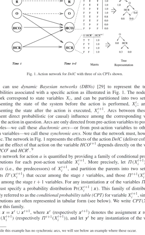
Fig. 1. Action network for DelC with three of six CPTs shown.

We can use dynamic Bayesian networks (DBNs) [29] to represent the transition probabilities associated with a specific action as illustrated in Fig. 1. The nodes in the network correspond to state variables Xi, and can be partitioned into two sets: those

representing the state of the system before the action is performed, X_it; and those representing the state after the action is executed, Xt_i+1. Arcs between these nodes represent direct probabilistic (or causal) influence among the corresponding variables under the action in question. Arcs are only directed from pre-action variables to post-action variables—we call these diachronic arcs—or from action variables to other post-action variables—we call these synchronic arcs. Note that the network must, however, be acyclic. The network in Fig. 1 represents the effects of the action DelC (deliver coffee). We see that the effect of that action on the variable HCOt+1depends directly on the variables Ot, HCOt and HCRt.9

The network for actiona is quantified by providing a family of conditional probability distributions for each post-action variable Xt_i+1. More precisely, let Π (X_it+1) be the

parents (i.e., the predecessors) of Xt_i+1, and partition the parents into two sets: those parents Πt(X_it+1) that occur among the stage t variables, and those Πt+1(Xt_i+1) that occur among the staget+1 variables. For any instantiationx of the variablesΠ (Xt_i+1), we must specify a probability distribution Pr(Xt_i+1|x). This family of distributions is usually referred to as the conditional probability table (CPT) for variableXt_i+1, since these distributions are often represented in tabular form (see below). We write CPT(Xi, a)to

denote this family.

Let x=xt ∪xt+1, where xt (respectivelyxt+1) denotes the assignment x restricted toΠt(Xt_i+1)(respectivelyΠt+1(Xt_i+1)), and letyt be any instantiation of the variables

{X_jt: X_jt ∈/Πt(X_it+1)}. The semantics of this family of conditional distributions is given by:

Pr Xt_i+1=x|xt,yt,xt+1, At=a=Pr X_it+1=x|x.

In other words, the distribution governing state variableXt+1_{when actionais performed} at stagetdepends on its parents; furthermore, once the state variablesΠ (Xt_i+1)are known, Xt_i+1is independent of other variables at staget.

Fig. 1 illustrates these points in a simple case of the DelC action, where there are no synchronic arcs. The family of conditional distributions for HCOt+1 is given by a table: for each instantiation of variablesOt, HCOt and HCRt, the probability that HCOt+1= > is provided.10 This CPT can be explained by observing that: if the owner has coffee prior to the action, she still has coffee after the action; if the robot has coffee and is in the office, it will successfully hand over the coffee with probability 0.8; and if the robot does not have coffee, or is in the wrong location, it will not cause its owner to have coffee. Notice that this representation allows one to specify the conditional effects of a stochastic action: the effect of an action on a specific variable can vary with conditions on the pre-action state.

The effect of the action onW (wet) is also shown, and is especially simple: the robot is wet (respectively dry) with probability one if it was wet (respectively dry) before the action was performed. This variable is said to persist under the action DelC. The effects on U,OandR are captured by similar persistence relations (not shown). Finally, the effect of DelC on HCR is explained as follows: if the robot attempts DelC when it is not in the office, there is a 0.7 chance a passerby will take the coffee; if the robot is in the office it will lose the coffee with certainty. Since there is a 0.8 chance of the user getting coffee, the 0.2 chance of the user not getting coffee can be attributed to spillage.

Because there are no synchronic arcs, the action’s effect on each of the state variables is independent, given knowledge of the stateSt. In particular, for any stateSt, we have

Pr Wt+1, Ut+1, Rt+1, Ot+1,HCRt+1,HCOt+1|St

=Pr Wt+1|StPr Ut+1|StPr Rt+1|StPr Ot+1|St

×Pr HCRt+1|StPr HCOt+1|St. (7)

Furthermore, the terms on the right-hand side rely only on the parent variables at timet; for example, Pr(Wt+1|St)=Pr(Wt+1|Π (Wt+1))=Pr(Wt+1|Wt). Thus, we can easily determine state transition probabilities given the compact specification provided by the DBN.

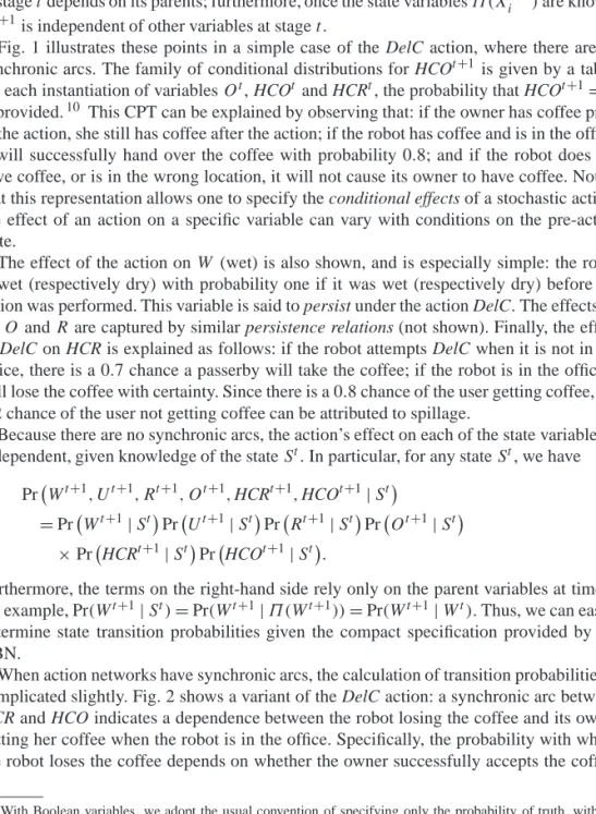
When action networks have synchronic arcs, the calculation of transition probabilities is complicated slightly. Fig. 2 shows a variant of the DelC action: a synchronic arc between

HCR and HCO indicates a dependence between the robot losing the coffee and its owner

getting her coffee when the robot is in the office. Specifically, the probability with which the robot loses the coffee depends on whether the owner successfully accepts the coffee: 10_{With Boolean variables, we adopt the usual convention of specifying only the probability of truth, with the} probability of falsity given by one minus this value.

Fig. 2. A modified action network for DelC with a synchronic arc.

if the owner gets the coffee, the robot loses it; but if the owner does not (or if she already had coffee), the robot loses the coffee with probability 0.2. Such synchronic dependencies reflect correlations between an action’s effect on different variables.

The independence of thet+1 variables givenStdoes not hold in DBNs with synchronic arcs. Determining the probability of a resulting state requires some simple probabilistic reasoning, for example, application of the chain rule.11 In this example, we can write

Pr HCRt+1,HCOt+1|St=Pr HCRt+1|HCOt+1, StPr HCOt+1|St.

The joint distribution overt+1 variables givenSt can then be computed with a slightly modified version of Eq. (7):

Pr Wt+1, Ut+1, Rt+1, Ot+1,HCRt+1,HCOt+1|St

=Pr Wt+1|StPr Ut+1|StPr Rt+1|StPr Ot+1|St

×Pr HCRt+1|HCOt+1, StPr HCOt+1|St. (8)

Notice that only the two variables HCR and HCO are correlated—the remaining independencies allow the computation to be factored with respect to the other four variables.

We make a few observations about this representation.

(1) Unlike normal Bayes nets or DBNs, we do not provide a marginal distribution over the pre-action variables. In solving fully observable MDPs, we are only concerned with the prediction of the resulting state distribution under some action given knowledge of the current state. As such, an action network provides a schematic 11_{Note that this rationale relies on the basic semantics Bayesian networks. Given two states s}

i and sj,

determining Pr(si, a, sj) involves simple table lookup and multiplication, the presence of synchronic arcs

representation of all|S|transition distributions: instantiating the pre-action variables to represent any statesallows the straightforward computation of Pr(·, a, s). (2) We must specify an action network for each action. In this way, an action

network can be seen as a compact specification of a transition matrix for that action. It is sometimes convenient to provide a single network with the choice of action represented as a variable, and the distributions over post-action variables conditioned on this action node. This type of representation, common in influence diagrams [69], can sometimes be more compact than a set of individual networks for each action (for example, when a variable’s value persists for most or all actions); see [15] for a discussion of the relative advantages of the two approaches. We will not consider the single network representation in this paper.

(3) Because of the Markov property, we need only specify the relationship between variablesXt andXt+1: knowledge of variablesXt_i−k (k >0) is irrelevant to the prediction of the values of variables Xt_j+1 given Xt_{. Furthermore, stationarity}

allows us to specify the dynamics schematically, with one DBN for each action characterizing its effects given stateSt for anyt>0.

(4) Typically, the DBN representation of an action is considerably smaller than the corresponding transition matrix. In the example above, the system has 26=64 states, hence each transition matrix requires the specification of 642 =4096 parameters. The DBN in Fig. 1 requires the specification of only 36 parameters, while that in Fig. 2 has only 64 parameters.12 We will see below that suitable representations of CPTs can make DBNs even more compact.

In the worst case, a “maximally connected” DBN will require the same number of parameters as a transition matrix. However, when the effects of actions exhibit certain regularities (e.g., they have the same effect on a given variable under a wide variety of circumstances) or when the effects on subsets of variables are independent, DBNs will generally be much more compact. See [11,15] for a more detailed discussion of this point. This representation (when augmented with the CPT representations described below) also compares favorably with probabilistic variants of STRIPSoperators with respect to representation size [11].

(5) In a certain sense, the DBN representation might be seen to fall prey to the

frame problem [55]: one must specify explicitly that a variable that is intuitively

“unaffected” by an action persists in value. In Fig. 1, for instance, an arc relating Wt and Wt+1, together with the corresponding CPT for Wt+1, are required so that one can infer thatWt+1 has the same value asWt (when DelC is executed). However, it is not hard to allow the specification of an action’s effects to focus only on those variables that change, leaving the distributions over unaffected variables unspecified. Such unspecified CPTs can be filled in by default, and unspecified arcs (e.g., the dashed arcs in Fig. 1) can be added automatically. The frame problem in DBNs (including aspects related to variables that change values under some conditions and not others) is discussed in detail in [15].

12_{If we exploit the fact that probabilities sum to one, we can remove one entry from each row of a transition} matrix and one from each row of a CPT (as we have done in the figures). In this case, a transition matrix would require 4032 entries, while the DBNs above have only 18 and 32 parameters, respectively.

3.1.2. Structured representations of conditional distributions

The DBN representation of an action a exploits certain regularities in the transition function induced by the action. Specifically, the effect ofa on a variableXi, given any

assignment of values to its parentsΠ (Xt_i+1), is identical no matter what values are taken by other state variables at timet (or earlier). However, this representation does not allow one to exploit regularities in the distributions corresponding to different assignments to Π (Xt_i+1).

We can view the CPT for variableXi in a DBN as a function mapping val(Π (Xt_i+1))—

the set of value assignments to Xi’s parents—into∆(val(Xi))—the set of distributions

over Xi. This function is traditionally represented in a tabular form: one explicitly lists

each assignment in val(Π (X_it+1))in a table along with the corresponding distribution for Xi(the tables in Figs. 1 and 2 are examples of this).

In many cases, this function can be more compactly represented by exploiting the fact that the distribution overXiis identical for several elements of val(Π (Xit+1)). For instance,

in the CPT for HCO in Fig. 1, we see that only three distinct distributions are mapped to from the eight assignments of HCO’s parents. This suggests that a more compact function representation for this mapping might be useful.

In this paper, we consider the use of decision trees [64] to represent these functions. The CPT for a variableXi in an action network will be represented as a decision tree: the

interior nodes of the tree are labeled with parents ofXi; the edges of the tree are labeled

with values of the parent variable from which those edges emanate; and the leaves of the tree are labeled with distributions forXi. The semantics of such a tree is straightforward:

the conditional distribution over Xi determined by any assignment x to its parents is

given by the distribution at the leaf node on the unique branch of the tree whose (partial) assignment to parent variables is consistent withx.

Examples of such trees are shown in both Figs. 1 and 2, next to the corresponding CPTs. The mapping from HCO’s parents into distributions over HCO in Fig. 1 is represented more compactly in the decision-tree format than the usual tabular fashion. The structure of the tree corresponds to our intuitions regarding the effects of DelC. If HCO was true, it remains true;13 but if HCO was false, then it becomes true with probability 0.8 ifOis true and HCR is true; otherwise it remains false. In a sense, decision trees reflect the “rule-like” structure of action effects. The tree for HCR in Fig. 2 relies on a synchronic parent.14

We focus on decision trees in this paper because of their familiarity and the ease with which they can be manipulated. Furthermore, they are often quite compact when used to describe actions. However, other representations may be suitable, and more compact, in certain circumstances. CPTs could sometimes be more compactly represented using rules [60,64], decision lists [65] or Boolean decision diagrams [19]. The algorithms we provide in the next section are designed to exploit the decision-tree representation, but we see no fundamental difficulties in developing similar algorithms to exploit these other

13_{We adopt the convention that, for Boolean variables, left edges denote>and right edges denote⊥.} 14_{Unless a node has synchronic parents, we will omittandt+1 superscripts at the interior node labels of the} decision-tree CPT; all such nodes will be understood to refer to variables at timet, nott+1.

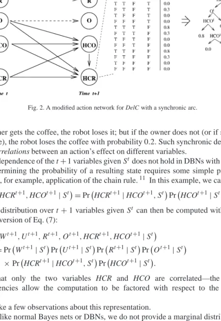
Fig. 3. The reward tree for the coffee example.

representations. Indeed, we will briefly point out extensions of the work described in this paper that exploit decision diagram representations.15

We note that this representation can be viewed as exploiting what is known as

context-specific independence in Bayesian networks [14]. Just as the independence of two variables

given knowledge of some subset of variables can be determined using the graphical structure of a Bayes net, additional independence can be inferred given certain assignments to a subset of variables (or a specific context). Algorithms for detecting these context-specific independencies using CPT representations such as decision trees and decision graphs are described in [14]. Related notions can be found in [38,59,70]. We note that

asymmetric representations of conditional distributions in influence diagrams have also

been proposed and investigated in [74].

3.2. Reward representation

Reward functions can be represented in a similarly compact fashion. Rather than specify a vector of reward valuesR(s)of size|S|, we can exploit the fact that reward is generally determined by a subset of system features. We represent the dependence of reward on specific state features using a diagram such as that shown in Fig. 3: here a reward node (the diamond in the figure) depends only on the values of the variablesW and HCO. The matrix represents this reward as function of the values taken by the two variables. Here we see that the best states are those in which the owner has coffee and the robot is dry, while the worst states are those in which the variables take the opposite values. Note that there is a preference for states in which the robot is wet and the owner has coffee over those where the robot stays dry and its owner is without coffee: thus, delivering coffee is a higher priority objective for the robot than staying dry.

The reward node in this example is related to the value nodes of influence diagrams [45, 69]. In influence diagrams, these nodes generally represent (long-term) value, whereas we use them to represent immediate reward (note that we assume stationarity of the reward process). In both cases, the independence of reward and certain state variables is exploited. Some work on influence diagrams has considered the use of reward nodes such as these, which are combined using some function (e.g., summation) to determine overall value (see, 15_{Deterministic, goal-based regression algorithms have been developed for such representations in many} circumstances; e.g., see [20] for a discussion of regression using Boolean decision diagrams. Decision-theoretic generalizations of these techniques, using ideas developed in the following section, should prove useful.

e.g., [79]). If action costs need to be modeled (i.e., reward has the formR(s, a)), a node representing the chosen action can be included, as they are in influence diagrams, or a separate reward function can be specified for each action, just as we specified a distinct DBN for each action to capture the process dynamics.

As with CPTs for actions, this conditional reward function can also be represented using a decision tree. In the example shown, the decision tree is no more compact than the full table; but in many instances, a decision-tree representation can be considerably more compact.

The representation of reward functions can sometimes be more compact if the reward function is comprised of a number of independent components whose values are combined with some simple function to determine overall reward. These ideas are common in the study of multi-attribute utility theory [49]. In our example, the reward function can be broken into two additive, independent components: one component determines the “sub-reward” determined by HCO—0.9 if HCO, 0 if HCO; and the other determines the sub-reward for W—0.1 of W and 0 if W. The reward at any state is determined by summing the two sub-rewards at the state. If there are a number of such component reward functions, specification of reward in terms of these components (together with a combination function) can often be considerably more compact.

While we permit a number of “independent” decision trees to be specified, our algo-rithms do not exploit the utility independence inherent in such a reward specification. In-stead, we simply combine the component functions into a single decision tree representing the true (global) reward function. How best to exploit such utility independence in MDPs in general is still an open question, though it has received some attention. For discussion of these issues, see [9,37,56,71].

3.3. Value function and policy representation

It is clear that value functions and policies can also be represented using decision trees (or other compact function representations). Again, these exploit the fact that value or optimal action choice may not depend on certain state variables, or may only depend on certain variables given that other variables take on specific values.

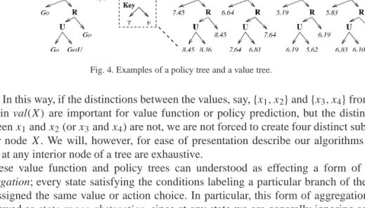
The algorithms we develop in the next section construct tree-structured representations of value functions and policies. Both value trees and policy trees have internal nodes labeled by state variables and edges labeled with (corresponding) variable values. The leaves of value trees are labeled with real values, denoting the value of any state consistent with the labeling of the corresponding branch. The leaves of policy trees are labeled with actions, denoting the action to be performed at any state consistent with the labeling of the corresponding branch. Tree representations of policies are sometimes used in reinforcement learning as well [23], though in a somewhat different fashion. Examples of a policy and value tree are given in Fig. 4.

In our implementation of decision-theoretic regression and structured dynamic program-ming algorithms described in the next section, we allow our trees to be slightly more so-phisticated in the case of multi-valued variables. When a tree splits on a variable with more than two domain values, we require only that the domain be split into two or more

Fig. 4. Examples of a policy tree and a value tree.

node. In this way, if the distinctions between the values, say,{x1, x2}and{x3, x4}from the domain val(X)are important for value function or policy prediction, but the distinction betweenx1andx2(orx3andx4) are not, we are not forced to create four distinct subtrees under nodeX. We will, however, for ease of presentation describe our algorithms as if splits at any interior node of a tree are exhaustive.

These value function and policy trees can understood as effecting a form of state

aggregation; every state satisfying the conditions labeling a particular branch of the tree

are assigned the same value or action choice. In particular, this form of aggregation can be viewed as state space abstraction, since at any state we are generally ignoring certain features and using only the value of others in predicting, say, the value or optimal action choice at that state. It is clear that similar remarks can be applied to both the DBN action representation, where states with similar dynamics under a specific action are grouped together, and to the decision-tree reward representation.

Categorizing these types of abstraction along the dimensions described in [11,30], our methods use nonuniform abstraction; that is, different features are ignored in different parts of the state space. In particular, these decision trees capture a conditional form of relevance, where certain variables are deemed to be relevant to value function prediction under certain conditions, but irrelevant under others. Compared to linear function approximators or neural network representations of value functions, our representations aggregate states in a “piecewise constant” fashion.

As we will see below, our abstraction scheme can also be classified as adaptive in that the aggregation of states varies over time as our algorithms progress. Finally, our main algorithm implements an exact abstraction process, whereby states are aggregated only when they agree exactly on the quantity being represented (e.g., value, reward, optimal action or transition distribution). We will see in Section 6.2 an approximate variant of this abstraction method.

4. Decision-theoretic regression

The decision-tree representations described in the previous section provide a means of representing value functions and policies more compactly than the straightforward table-based representations. In particular, if a tree can be constructed to represent the optimal value function or policy in which the number of internal nodes labeled by state variables

is polynomial in the number of variables, then this representation will be exponentially smaller than the corresponding tabular representation. If we were given the structure of such a tree for (say) the value function by an oracle, one might imagine partitioning state space into the abstract states given by the structure of the tree, and performing dynamic programming—let’s assume value iteration—over the reduced state space. In this case, each dynamic-programming iteration would require only one Bellman backup per abstract state, thus, a number of backups which is a polynomial function of the logarithm of the number of states.

Unfortunately, even if the true value function can be compactly represented using a decision tree, the regions of state space over which an intermediate value function generated by value iteration is constant need not match those of the optimal value function. Furthermore, we don’t usually have access to oracles who provide us with suitable abstractions. What we need are algorithms that, for example, infer the proper structure of the sequence of value functions produced by value iteration, and perform Bellman backups once per abstract state once this structure has been deduced. One could use similar ideas in (regular or modified) policy iteration.

In this section we develop methods to do just this. These techniques exploit the structure inherent in the MDP that has been made explicit by the DBN and decision-tree representations of the system dynamics and the reward function. Specifically, given a tree-structured representation of a value functionV, we derive algorithms that produce tree-structured representations of the following functions: Q-functions with respect toV; the value function obtained by performing a Bellman backup with respect toV; the value function obtained by successive approximation with respect to a fixed policyπ, whereπis represented with a decision tree; and the greedy policy with respect toV. These algorithms infer (to varying degrees) the appropriate structure of the underlying value function or policy before performing any decision-theoretic calculations (e.g., maximizations or expected value calculations). In this way, operations such as computing the expected value of an action are computed only once per abstract state (or region of state space, or leaf of the tree), instead of once per system state. If the size of the trees is substantially smaller than the size of the original state space, the computational savings can also be substantial. The key to all of the operations mentioned above is the first—the computation of a Q-functionQV_a for actionawith respect to a given value functionV. This operation can be viewed as the decision-theoretic analog of regression, as described in Section 1.1.

In this section, we assume that none of the action networks describing our domain contain synchronic arcs; that is, an action’s effects on distinct variables are uncorrelated (given knowledge of the current state). This assumption is valid in many domains, including those we experimented with, but may be unrealistic in others. We do this primarily for reasons of exposition. Our algorithms are conceptually simple in the case where correlations are absent. As described in Section 3.1.1, determining the probability of a state variable taking a certain value after an action is performed is straightforward. When the action network has no synchronic arcs, these can be combined by multiplication to determine state transition probabilities due to their independence; but this combination requires some simple probabilistic inference when synchronic arcs are present. To avoid having the intuitions get lost in the details of this inference, we present our algorithms

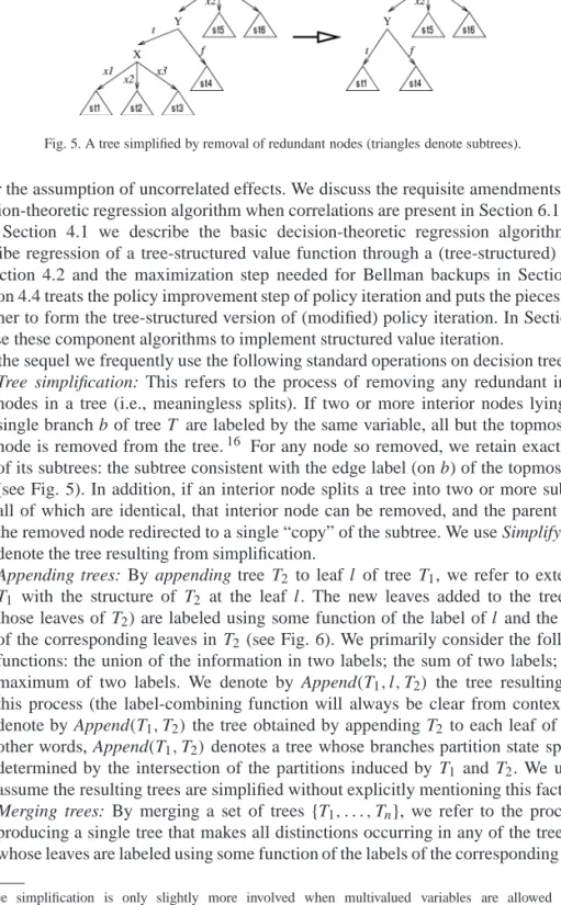
Fig. 5. A tree simplified by removal of redundant nodes (triangles denote subtrees).

under the assumption of uncorrelated effects. We discuss the requisite amendments to the decision-theoretic regression algorithm when correlations are present in Section 6.1.

In Section 4.1 we describe the basic decision-theoretic regression algorithm. We describe regression of a tree-structured value function through a (tree-structured) policy in Section 4.2 and the maximization step needed for Bellman backups in Section 4.3. Section 4.4 treats the policy improvement step of policy iteration and puts the pieces above together to form the tree-structured version of (modified) policy iteration. In Section 4.5 we use these component algorithms to implement structured value iteration.

In the sequel we frequently use the following standard operations on decision trees:

• Tree simplification: This refers to the process of removing any redundant interior

nodes in a tree (i.e., meaningless splits). If two or more interior nodes lying on a single branchbof treeT are labeled by the same variable, all but the topmost such node is removed from the tree.16 For any node so removed, we retain exactly one of its subtrees: the subtree consistent with the edge label (onb) of the topmost node (see Fig. 5). In addition, if an interior node splits a tree into two or more subtrees, all of which are identical, that interior node can be removed, and the parent arc of the removed node redirected to a single “copy” of the subtree. We use Simplify(T )to denote the tree resulting from simplification.

• Appending trees: By appending tree T2 to leafl of tree T1, we refer to extending

T1 with the structure of T2 at the leaf l. The new leaves added to the tree (i.e., those leaves ofT2) are labeled using some function of the label ofl and the labels of the corresponding leaves inT2 (see Fig. 6). We primarily consider the following functions: the union of the information in two labels; the sum of two labels; or the maximum of two labels. We denote by Append(T1, l, T2) the tree resulting from this process (the label-combining function will always be clear from context). We denote by Append(T1, T2)the tree obtained by appendingT2to each leaf ofT1. In other words, Append(T1, T2)denotes a tree whose branches partition state space as determined by the intersection of the partitions induced by T1 andT2. We usually assume the resulting trees are simplified without explicitly mentioning this fact.

• Merging trees: By merging a set of trees {T1, . . . , Tn}, we refer to the process of

producing a single tree that makes all distinctions occurring in any of the trees, and whose leaves are labeled using some function of the labels of the corresponding leaves 16_{Tree simplification is only slightly more involved when multivalued variables are allowed to split} nonexhaustively. In this case, a certain variable may legitimately appear on a branch of a tree more than once, not unlike continuous splits in classification and regression trees.

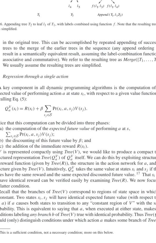
Fig. 6. Appending treeT2to leafl1ofT1, with labels combined using functionf. Note that the resulting tree has been simplified.

in the original tree. This can be accomplished by repeated appending of successive trees to the merge of the earlier trees in the sequence (any append ordering will result in a semantically equivalent result, assuming the label-combination function is associative and commutative). We refer to the resulting tree as Merge({T1, . . . , Tn}).

We usually assume the resulting trees are simplified.

4.1. Regression through a single action

A key component in all dynamic programming algorithms is the computation of the expected value of performing actionaat statesi, with respect to a given value functionV.

Recalling Eq. (5): QV_a(si)=R(si)+β

X

sj∈S

Pr(si, a, sj)V (sj).

Notice that this computation can be divided into three phases:

(a) the computation of the expected future value of performing_P aats,

sj∈SPr(si, a, sj)V (sj);

(b) the discounting of this future value byβ; and (c) the addition of the immediate rewardR(si).

IfV is represented compactly using Tree(V ), we would like to produce a compact tree-structured representation Tree(QV_a)ofQV_a itself. We can do this by exploiting structure in the reward function (given by Tree(R)), the structure in the action network fora, and the structure given by Tree(V ). Intuitively,QV_a takes the same value at statessi andsj if these

states have the same reward and the same expected discounted future value.17 Thatsi and

sj have identical reward can be verified easily by examining Tree(R). We now focus on

the latter condition.

Recall that the branches of Tree(V ) correspond to regions of state space in whichV is constant. Two statessi, sj will have identical expected future value (with respect toV

anda) ifa causes both states to transition to any “constant region ofV” with the same probability. This is equivalent to saying thata, when executed at either state, makes the conditions labeling any branchbof Tree(V )true with identical probability. Thus Tree(QV_a) should (only) distinguish conditions under which actionamakes some branch of Tree(V )

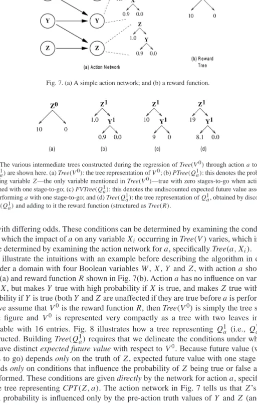
Fig. 7. (a) A simple action network; and (b) a reward function.

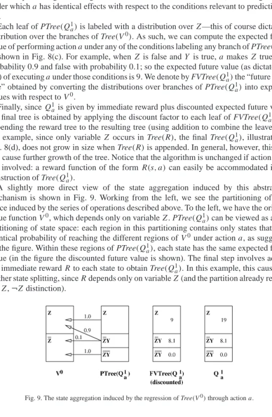
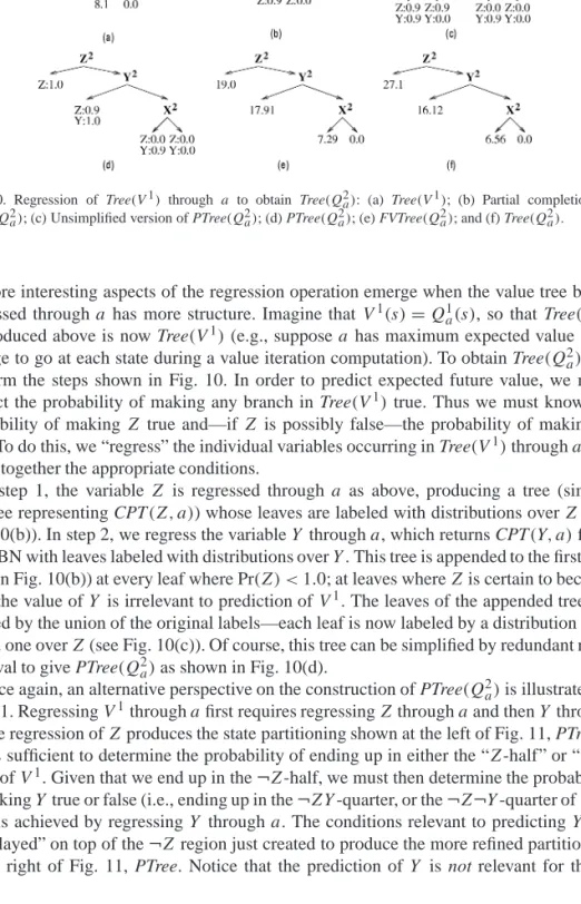
Fig. 8. The various intermediate trees constructed during the regression of Tree(V0)through actionato obtain

Tree(Q1a)are shown here. (a) Tree(V0): the tree representation ofV0; (b) PTree(Q1a): this denotes the probability

of making variableZ—the only variable mentioned in Tree(V0)—true with zero stages-to-go when actionais performed with one stage-to-go; (c) FVTree(Q1_a): this denotes the undiscounted expected future value associated with performingawith one stage-to-go; and (d) Tree(Q1_a): the tree representation ofQ1_a, obtained by discounting

FVTree(Q1_a)and adding to it the reward function (structured as Tree(R).

true with differing odds. These conditions can be determined by examining the conditions under which the impact ofaon any variableXioccurring in Tree(V )varies, which in turn

can be determined by examining the action network fora, specifically Tree(a, Xi).

We illustrate the intuitions with an example before describing the algorithm in detail. Consider a domain with four Boolean variablesW,X,Y andZ, with actiona shown in Fig. 7(a) and reward functionRshown in Fig. 7(b). Actionahas no influence on variables W orX, but makesY true with high probability ifX is true, and makesZtrue with high probability ifY is true (bothY andZare unaffected if they are true beforeais performed). If we assume thatV0_{is the reward functionR, then Tree(V}0_{)is simply the tree shown} in the figure and V0 _{is represented very compactly as a tree with two leaves instead} of a table with 16 entries. Fig. 8 illustrates how a tree representing Q1_a (i.e., QV_a0) is constructed. Building Tree(Q1_a)requires that we delineate the conditions under whicha will have distinct expected future value with respect toV0. Because future value (with 0 stages to go) depends only on the truth of Z, expected future value with one stage to go depends only on conditions that influence the probability ofZ being true or false aftera is performed. These conditions are given directly by the network for actiona, specifically by the tree representing CPT(Z, a). The action network in Fig. 7 tells us thatZ’s post-action probability is influenced only by the pre-post-action truth values of Y andZ (and that