Optimised decision-making under grade uncertainty in surface mining

Department of Mathematics & Statistics

Optimised Decision-Making under Grade

Uncertainty in Surface Mining

Francois Grobler

This thesis is presented for the Degree of Doctor of Philosophy

of

Curtin University

To the best of my knowledge and belief this thesis contains no material previously published by any other person except where due acknowledgement has been made.

This thesis contains no material which has been accepted for the award of any other degree or diploma in any university.

Signature: Date:

finds uncertainty fascinating.”

- Carl von Clausewitz

“Information is the resolution of uncertainty.”

Firstly, I would like to thank my supervisor, Lou Caccetta for his support and encouragement during this journey.

I also want to thank my associate supervisor, Jose Saavedra-Rosas, for his inputs and guidance around the thesis structure, mathematical modelling and programming in Python as well as acting as a constructive critic for my often exotic and tangential ideas - he usually managed to reel me back in although not always without a lively exchange of thoughts...

Most importantly, to my wife C´eline, for tolerating the last four years and for being a willing (mostly) sounding board for new ideas, sometimes responding with a stifled yawn but always with a supporting ear.

I would also like to thank CAE Mining for providing the conditional simulation data sets which have been used for a major part of this thesis.

Planners and managers tasked with strategic open pit scheduling in real indus-trial situations are faced with two key dilemmas.

Firstly, finding optimal answers for the Open Pit Production Scheduling Prob-lem requires the solution of large combinatorial optimisation probProb-lems. Unfor-tunately, and despite a lot of effort, progress has been slow in finding ways to solve these large problems satisfactorily (or at all) in a reasonable amount of time through mathematical programming approaches.

The second issue is that until recently, most analysts and planners have relied on deterministic inputs to their models and have ignored parameter uncertainty. In doing this they have assumed in effect that information related to geological and grade variability, as well as the future behaviour of commodity prices and other economic factors (amongst many others), are known at the time that the decision is made. In reality these inputs are highly uncertain and depending on which specific instances are selected, could lead to vastly different results in pit designs and mining schedules.

With reference to the first issue, the size problem is commonly dealt with by either reducing the size of the input data set or by implementing clever formula-tion and soluformula-tion strategies.

From the data perspective, a quick and easy strategy with drastic effects is to remove such data from the model upfront which are superfluous from a geo-metric point of view. In other cases, an attempt is made to lift the burden of dealing with large models by re-blocking or aggregating blocks into data sets with a smaller more manageable number of blocks. This makes it easier to solve the problem but potentially dilutes the resolution of the input data and results.

From the solution angle, heuristic methods are often used to solve large models faster than exact mathematical methods but this sacrifices accuracy and the abil-ity to prove optimalabil-ity. Some encouraging advances have been made over the last decade using mathematical programming methods such as mixed integer linear programming (MILP) in the formulation and solving of the problem without jeop-ardising the resolution of the input data. Key improvements include intelligent data pre-processing, removing obsolete variables with respect to earliest and lat-est start times, the use of branching algorithms with relaxed integer constraints, exploiting strong branching characteristics of the problem, the introduction of im-proved cutting planes, and decomposition methods such as Lagrangian relaxation. The second problem (input uncertainty) has received less attention. A promis-ing simulation method (Conditional Simulation) has enabled decision makers in the mining industry to generate multiple realisations representing the spatial vari-ability of geological features and attributes such as metal grades and densities of a deposit. When such simulations are considered together they provide insights into the estimation of the uncertainty inherent in the geological or grade model due to limited information. Similarly, the stochastic behaviour of commodity prices resulting in limitations in accurate forecasting has been captured by meth-ods such as Monte Carlo simulation and Real Option Valuation.

Unfortunately many of these methods, although bestowing massive improve-ments compared to historical deterministic models, still result in multiple out-comes (or scenarios) which ultimately leave the decision maker with the dilemma of having to select the best option.

In this thesis we first draw on some basic advancements made in the field of mathematical programming to construct a simplistic MILP formulation for a small instance of the Open Pit Production Scheduling Problem. We then in-troduce multiple Conditional Simulation data sets which are successively solved using the MILP formulation generating candidate solutions to the problem. We also introduce an interpretative framework which compares average values against accompanying standard deviation. We combine these two metrics into a single indicator, the coefficient of variation (CV), which we propose to be used to find a suitable trade off between risk (standard deviation of values) and return (average of values). This metric can then be used to make sense of candidate solutions and

optimisation results derived from multiple grade instances based on Conditional Simulations. This framework enables the identification of a single or a select number of most ’attractive’ options by considering the trade off between risk and return (expressed as the CV).

We then use a version of the MILP formulation to incorporate a Scenario Op-timisation approach which was developed in the 90’s and applied to projects in power generation and financial portfolio optimisation. The approach can be used to solve a stochastic model based on a particular method for combining scenario solutions into a single feasible and ’robust’ strategy. The results from this ap-proach are then similarly tested for viability by using the interpretive framework. This thesis combines advancements made in exact mathematical methods with a probabilistic scenario optimisation approach which incorporates and considers grade uncertainty while arriving at a single ’best’ or most attractive solution (al-though not necessarily highest value or lowest risk). The resultant methodology is tested on a case study of 40 conditional simulations.

The three key contributions of this thesis are: 1. Scenario Optimisation

By combining an exact deterministic MILP optimisation approach based on Caccetta and Hill (2003) with multiple conditional simulation inputs we utilised a modified two-stage scenario optimisation approach to generate a unique solution to an open pit scheduling case study.

This approach has an initial stage during which optimised solutions are generated using a MILP objective function maximisation. This is then followed in a second stage by finding a solution which minimises the sum of the absolute differences between the original solutions derived in stage one and the current solution applied to the equivalent simulation data set. This two-stage scenario optimisation approach was modified from Dembo (1992) who used it in financial portfolio optimisation and in hydroelectric power generation. Our research indicates that this is the first time this approach has been used in a mining context.

In order to incorporate both risk minimisation and value maximisation into the decision making criteria when comparing various ‘competing’ candidate solutions, we developed an interpretive framework which utilises the coef-ficient of variation (CV) as a measure which includes both factors. The framework based on the CV enables comparison of multiple optimisation results and their associated statistics when compared against the underly-ing data. Further, it provides an intuitive and easy way of identifyunderly-ing those solutions that offer a favourable trade-off between risk and return.

Although the coefficient of variation is a well known statistical metric for normalising and comparing different scenarios and options with different means and standard deviations, our research indicates that this is the first time the CV has been used in such an interpretive framework and certainly the first time it has been used in the mining context for comparing optimi-sation solutions derived from conditional simulations.

3. Data Perturbations

We conducted early exploratory research with a concept that we call ‘data perturbation’ and that we believe has a lot of merit for further research and investigation.

Generally, a number of ways can be utilised to generate valid candidate mining schedules. These can be as basic as starting from the top of a deposit and mining naively downwards bench by bench, and as sophisticated as following a true holistically optimised solution.

As long as certain requirements are fulfilled, such as adherence with prede-termined precedence constraints (or pit slope angles) and compliance with minimum and maximum annual production capacity constraints, any such schedule will qualify as a ‘valid’ solution. Of course it could be a partic-ularly poor economic solution (it might even have a negative NPV) but it would be permissible as a solution.

One way of generating such a permissible solution is to use a slightly per-turbed version of the underlying conditional simulation data set to gener-ate an optimised solution. This can for instance be achieved by applying a small random modifying factor (for example a uniformly selected factor that varies between -5 and +5 percent) on the true block value.

Although such a modification is not permitted in generating valid condi-tional simulation data sets during geo-statistical estimation, it could

never-theless be used as the basis for an optimised schedule. When such a solution is then compared against the underlying true condition simulation data, it might lead to improvements in the CV and therefore provide a more attrac-tive solution than those derived directly from solving conditional simulation datasets, or those derived via scenario optimisation approach.

We believe this approach is a unique way of generating a large number of ‘inexpensive’ candidate solutions which can be assessed for incremental improvements in value or CV. As this method arose as an outflow of our research relatively late in the thesis time-frame we could only conduct cur-sory exploration on it but we believe that it merits further investigation and research.

Acknowledgements vii Abstract ix 1 Introduction 1 1.1 Overview . . . 1 1.2 Problem statement . . . 3 1.3 Previous research . . . 3

1.4 Research Objectives and Motivation . . . 4

1.5 Research Methodology . . . 4

1.6 Areas of Application . . . 5

1.7 Organisation of the thesis . . . 7

2 Open Pit Production Scheduling 9 2.1 Introduction . . . 9

2.2 Mining operations . . . 9

2.2.1 Mining methods . . . 9

2.2.2 Mining activities . . . 10

2.3 Data collection and interpretation . . . 11

2.3.1 Drilling, sampling and geological modelling . . . 11

2.4 Geostatistics . . . 11

2.4.1 Creating a block model . . . 15

2.5 Geological and Mining Uncertainty . . . 19

2.5.1 General Sources of Mining Risk . . . 20

3 Literature Review 22 3.1 Introduction . . . 22

3.2 Deterministic Mine Planning and Scheduling Methodologies . . . 22

3.2.2 Integrated modelling approach . . . 29

3.3 Probabilistic and Stochastic methods . . . 34

3.3.1 Background . . . 34 3.3.2 Geological uncertainty . . . 36 3.3.3 Conditional Simulation . . . 37 3.3.4 Stochastic Programming . . . 41 3.3.5 Scenario Optimisation . . . 42 4 MILP formulation 43 4.1 Introduction . . . 43 4.2 Preliminaries . . . 44 4.2.1 Mathematical Modelling . . . 44 4.2.2 Branch-and-bound Algorithm . . . 44

4.3 Data Pre-processing and Optimisation Settings . . . 46

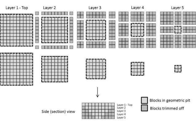
4.3.1 Geometric (rectangular) Trimming . . . 46

4.3.2 Realisitic MIP gap setting . . . 50

4.4 MILP Model Formulation . . . 56

4.4.1 Hardware and Software Considerations . . . 56

4.4.2 Data . . . 56

4.4.3 Assumptions . . . 60

4.4.4 Variables, Constraints and Objective Function . . . 62

4.4.5 Formulation . . . 63 4.5 Case Study . . . 65 4.5.1 Background . . . 65 4.5.2 Assumptions . . . 65 4.5.3 Results . . . 66 4.6 Conclusion . . . 69

5 Introducing Risk and Uncertainty 71 5.1 Introduction . . . 71

5.2 Preliminaries . . . 72

5.2.1 Risk, Uncertainty and Variability defined . . . 72

5.2.2 Simulation . . . 76

5.3 Optimisation using Conditional Simulations . . . 80

5.4 Conditional Simulation Case Study . . . 82

5.4.1 Conventional application of Conditional Simulation . . . . 83 5.4.2 Interpretive Framework for considering Risk-Reward trade-off 90

5.5 Conclusion . . . 100

6 Scenario Optimisation 101 6.1 Introduction . . . 101

6.2 Preliminaries . . . 102

6.2.1 Formulation using Dembo’s approach . . . 104

6.3 Our Scenario Optimisation Formulations . . . 106

6.3.1 Scenario maximisation formulation . . . 106

6.3.2 Scenario minimisation formulation . . . 108

6.4 Case study . . . 110

6.5 Conclusions . . . 113

7 Conclusions and Recommendations 115 7.1 Conclusions . . . 115

7.1.1 MILP formulation . . . 116

7.1.2 Conditional Simulation and Interpretive Framework . . . . 117

7.1.3 Scenario Optimisation . . . 117

1.1 Flow diagram . . . 6

2.1 Open pit mine . . . 10

2.2 Geological interpretation from drill hole data . . . 12

2.3 Typical (idealised) Spherical Variogram . . . 13

2.4 Kriged vs. Conditionally Simulated models illustrating smoothing effect . . . 14

2.5 Three-dimensional geologic block model representation of blocks (cubes) in a deposit . . . 15

2.6 Example open pit configurations for two general types of deposit . 19 3.1 Nested pits illustrating parametrisation - section view length-wise through block model . . . 27

3.2 Bench-push back units - section view length-wise through block model . . . 28

3.3 (a) Kriged estimate v.s. (b to d) Simulations - source: Saave-dra Rosas (2009) . . . 37

4.1 Block precedences in 2-D section . . . 46

4.2 Edge trimming by level . . . 48

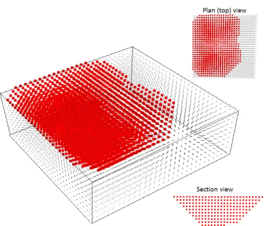
4.3 Case study - optimised Ultimate Pit . . . 50

4.4 Solution progression for case study 1 . . . 53

4.5 Solution progression for case study 2 . . . 54

4.6 Increase in X, Y and Z from origin (0,0,0) . . . 57

4.7 Block precedences . . . 61

4.8 Block precedences using ‘knight’s move’ pattern . . . 62

4.9 Perspective view of Marvin deposit . . . 66

4.10 Marvin distribution of grade ranges . . . 67

4.13 Marvin CPLEX - MIP progression . . . 68

4.12 Marvin CPLEX - optimisation strategy . . . 69

4.14 Marvin CPLEX - optimisation results . . . 69

5.1 Uncertainty (A) and Variability (B) in geology . . . 73

5.2 Statistic to demonstrate central tendency - source: Mun (2006) . . 75

5.3 Statistic to demonstrate spread - source: Mun (2006) . . . 75

5.4 Random walk generation of conditional simulation data points . . 78

5.5 Various estimation point selection approaches . . . 79

5.6 Comparing each Schedule against each Conditional Simulation . . 81

5.7 Ten example Conditional Simulations from 40 . . . 82

5.8 Schedule optimisations . . . 85

5.9 Schedule optimisations compared against simulations . . . 86

5.10 Statistical analysis for NPVs ($M) from schedule optimisations . . 88

5.11 Key statistics for schedules when tested against simulations . . . . 89

5.12 Sorting of schedules according to decreasing value . . . 91

5.13 Sorting of schedules according to increasing risk . . . 92

5.14 CV plotted for each schedule comparison . . . 93

5.15 CV plotted for each schedule comparison - sorted on increasing CV 94 5.16 Rescaling effect on Ave value and Std deviation . . . 95

5.17 Rescaling effect on CV (showing Unit or Normalised CV as NCV) 95 5.18 Risk against return . . . 96

5.19 Upside potential ratio . . . 99

6.1 Schematic of Scenario Optimisation showing Stages 1 and 2 . . . . 103

6.2 Scenario maximisation . . . 107

6.3 Two-stage scenario minimisation . . . 109

6.4 Schedule optimisations . . . 111

6.5 Results . . . 112

7.1 Generation of candidate solutions and testing for improved solu-tions using interpretive framework . . . 121

7.2 Candidate solutions generated through perturbations and testing using interpretive framework . . . 123

4.1 Rectangular trimming per level . . . 49

4.2 Technical assumptions for MIP gap case studies . . . 52

4.3 Example conversion of original to unit coordinates . . . 58

4.4 Optimisation parameters used for Marvin case study . . . 66

5.1 Schedule 1 evaluated against all 40 conditional simulation data sets (NPVs in $ m in brackets) . . . 87

5.2 Comparison of most attractive option from a value and risk per-spective . . . 93

5.3 Comparison of most attractive option from a value and risk per-spective . . . 94

Introduction

This chapter provides the context for the rest of the thesis. Within this chapter we lay out in basic terms:

(a) a brief description of the problem and the environment in which it occurs (Section 1.1),

(b) the key issues that we would like to address in the thesis (Section 1.2), (c) some of the main classical and recent research literature generated on the

key topics of interest (Section 1.3),

(d) the objectives that we aim to achieve through this research (Section 1.4), (e) what is the motivation for this line of research (Section??),

(f) the methodologies that will be followed to answer the questions raised (Sec-tion 1.5),

(g) areas where the findings and conclusions from this research can find prac-tical or commercial application (Section 1.6), and

(h) what we plan to achieve from each subsequent chapter in this thesis (Section 1.7).

1.1

Overview

Mining decisions related to large open pits mined over tens or even hundreds of years can be massively complex and involve a myriad of different components and

considerations. There are many areas within such operations where Operations Research in general and optimisation techniques specifically can be successfully in-troduced to gain the maximum benefit. These techniques are mostly implemented on the development and exploitation stages of mining projects and operations. Areas of application include ore-body modelling and ore reserve estimation, the design and scheduling of optimum pits, determining optimum blends and cut off policies, equipment maintenance and fleet optimisation studies to name but a few.

This thesis however occupies itself with the Open Pit Mining Production Scheduling Problem. A strategic solution to this particular problem involves the decision on:

(a) which of the available blocks in a mining block model to extract by surface mining methods (i.e. mine them or leave them in the ground),

(b) when (in which time period) should the extraction take place, and

(c) what to do with them (send a mined block to waste, to the processing plant for treatment or to a stockpile for later consideration).

All these decisions need to be made with the objective of maximising the economic value of such an exercise while satisfying safe wall-slope (precedence) restrictions, production capacity, market factor and environmental constraints.

Problems such as these are routinely formulated as mathematical models with pre-determined input values, decision variables and technical or capac-ity constraints. Such problems are then solved as linear programming (LP) or integer/mixed-integer programming (IP or MIP) formulations using commercial software.

One of the key limitations of these models is the high level of uncertainty in the input values (e.g. prices and ore/metal grades) and assumptions used to construct the models originally as well as the extent to which this is taken into account or ignored. In some cases this can be further exacerbated due to the size of the models and the number of variables required to be solved for models reaching anything close to realistic sizes.

1.2

Problem statement

The issue that we are trying to address in relation to the uncertainty problem can be stated as follows:

Many of the current mine scheduling optimisation approaches ignore the un-certainty around input data (e.g. grade values, density) thus failing to assess the inherent risk or robustness of derived solutions. Often when they do incorporate risk through methods like Conditional Simulation, they provide no method to interpret results or isolate a single or few most suitable options.

1.3

Previous research

Over the last few decades the Open Pit Mine Production and Scheduling Problem has been approached from many angles. Sequential methods divide the problem into components by first generating a solution to the ultimate pit problem, fo-llowed by generating periodic phases (also called ‘push backs’) and only then finding schedule solutions to the individual subcomponents. Pioneering work using a sequential approach and focussing on solving the ultimate pit problem was done by Lerchs and Grossmann (1964) in the 60’s using Graph Theory, Dynamic Programming and Network Flow methods. Numerous researchers subsequently built on 2-D and 3-D versions and modifications of Lerchs and Grossman’s original work. Original literature utilising a Network Flow method was proposed by Picard (1976) and expanded on by various others. Heuristic methods have also been used to solve the ultimate pit problem with one of the most well known being the Moving (Floating) Cone Method. Early solutions using the Moving Cone Method were proposed by David et al. (1974) and Lemieux (1979) and modifications to the method has been proposed by many others.

More holistic or integrated methods considered the problem as a whole and attempted to solve the problem without subdivision into parts. These meth-ods include linear (LP) and mixed integer linear programming (MILP) methmeth-ods combined with solution strategies such as branch and bound and cut generation, as well as decompositions methods such as Lagarangian relaxation. Key liter-ature from within this genre include Caccetta and Hill (2003), Gaupp (2008), Askari-Nasab et al. (2010), Darby-Dowman and Wilson (2002), Ramazan and Dimitrakopoulos (2004), Gershon (1982) and Weintraub et al. (2008).

Compared to the volume of work done on deterministic mine planning and schedule optimisation, research done on introducing uncertainty into mine

plan-ning has been relatively sparse. Since the early 90’s Dimitrakopoulos and various contributors have been exploring the use of Conditional Simulation as a way to incorporate uncertainty into the ultimate pit design and production schedul-ing problem e.g. Journel and Huijbregts (1978), Dimitrakopoulos (1990), Dimi-trakopoulos (1994) and Armstrong and Dowd (1994).

An interesting approach for incorporating uncertainty using Scenario Optimi-sation was suggested by Ron Dembo (Dembo, 1992) in the 90’s but never applied to the mining industry. In this thesis we build on his approach.

1.4

Research Objectives and Motivation

The primary objective of this study can be stated as:

To devise an effective method which enables the inclusion of geological (grade) uncertainty into the problem formulation to derive a risk-adjusted ‘robust’ solu-tion (i.e. a solusolu-tion that involves and acceptable trade off between risk and return) and to develop an interpretive framework to make sense of the results as an aid to decision making.

The motivation for this research is that grade variability and uncertainty is routinely ignored in the compilation of mine planning models. In the cases where grade risk is introduced through conditional simulations, the exercise involves the generation of multiple simulations with limited sense-making occurring in the interpretation of the results often still leaving the decision maker with multiple options without the capacity to select the ‘best’ or most attractive solution(s).

1.5

Research Methodology

The research methodology is as follows:

(a) Review literature and approaches used in the past to deal with the primary problem under review.

(b) For a suitable base metal deposit, formulate a deterministic MILP model for a small to medium size block model (1,000 to 50,000 blocks) based on pre-vious research and solve the problem using a commercial solver (CPLEX). Perform pre-processing on input data in order to reduce the size of the block model and data inputs as much as possible.

(c) Generate or obtain a block model which includes a suitable number of con-ditional simulations representing multiple equi-probable interpretations of the block model data.

(d) Generate a probabilistic modelling framework enabling iterative MILP op-timisations of conditional simulations recoding schedules derived

(e) Develop an interpretive framework with which to conduct comparative anal-ysis of derived options (schedules) in order to find a most suitable (‘robust’) solution which considers both value and risk.

(f) Investigate other approaches to incorporate model uncertainty in the solu-tion (e.g. scenario optimisasolu-tion) - add these solusolu-tions to the interpretative framework to see how they compare with schedules derived through opti-mising conditional simulation data sets.

1.6

Areas of Application

The key components of the mine planning process are illustrated in the following flow diagram (see Figure 1.1). Five areas have been identified within the optimi-sation set-up and solution process where it is believed that enhancements to the process can add significant value to the quality, solution time and interpretation of an optimisation.

1. Area A - during the pre-processing stage (see Chapter 4.3):

(a) the size of the problem (data) can be significantly reduced by consid-ering (and excluding) redundant blocks which can structurally not be part of the solution due to their geo-spatial location.

(b) some waste blocks can be excluded from the bottom layers of the block model since they do not add value to the solution and will therefore never be selected anyway.

2. Area B - during the model generation stage (see Chapter 4.4):

(a) blocks could be excluded during the variable declaration stage or as added constraints based on earliest and latest available start times.

Figure 1.1: Flow diagram

(b) such constraints are possible as a result of the combination of annual maximum/minimum mining capacity constraints and precedence con-straints.

3. Area C - during the optimisation (solve) stage (see Chapter 4.4):

(a) select realistic MIP gap settings (e.g. 1% to 5%) for the optimiser (e.g. CPLEX)

(b) select realistic CPU time or iterations as termination criteria for the optimiser

(c) select realistic memory capacity allocation

4. Area D - during an iterative stage between solution and redefining the model:

(a) during an iterative approach such as branch and cut where the opti-miser is used to solve only the relaxed LP (and not the MIP) strategies can be introduced to reduce the solution space via additional con-straints as the optimisation results are returned.

(b) using call back facilities additional constraints, cuts, node priorities etc. can systematically be introduced.

5. Area E - during interpretation of results (see Chapter 5.4):

(a) sense making going beyond just basic descriptive statistical summaries of the generated outputs

(b) developing an interpretive framework which clearly produces a way to disseminate and visualise results

(c) an interpretive framework which assists in identifying a single (or a select few) most favoured option.

1.7

Organisation of the thesis

The rest of this thesis is organised as follows:

Chapter 2 defines general mining terminology and then focuses on concepts specific to the open pit environment, geo-statistics and block modelling.

Chapter 3 provides a literature review focussing on research related to open pit optimisation following sequential and integrated approaches. This section includes various mathematical (‘exact’) and heuristic methods that researchers have developed to formulate and solve the Open Pit Production Scheduling Prob-lem with special focus on ways to deal with the model size probProb-lem. A second section of this chapter reviews literature related to the introduction of variable and parameter uncertainty via probabilistic or stochastic methods.

Chapter 4 details the formulation of a MILP model and applies a number of known strategies to improve the manageability or solvability of the model. These include data preprocessing strategies to reduce the size of the data set, as well

as model formulation and optimiser settings. A model is built in the Python (Pyomo)/CPLEX environment and solved, validated and interpreted.

Chapter 5 considers the introduction of grade uncertainty into the open pit optimisation problem through the use of Conditional Simulations. The chapter proceeds to develop an Interpretive Framework which enables a decision-maker to make sense of results derived from developing schedules from Conditional Simu-lations and testing them against the range of Conditional Simulation input data. The approach defines a strategy for integrating risk and return (the risk/return trade-off) by using the Coefficient of Variation of the resultant solution values as a metric thus proposing a method to identify the most attractive candidate solutions.

Chapter 6 considers a number of scenario optimisation techniques for in-cluding uncertainty, building on the research of Dembo (1992) and others. The chapter expands on various ways to develop models which recognise the variability introduced by conditional simulations. The two scenario optimisation approaches tested derive unique solutions which respectively minimises the average deviation from the expected value and maximises the average value of the solution. This method is tested against the Interpretive Framework developed in the previous section.

Chapter 7 provides a summary of the results and conclusions of the thesis and proposes some interesting areas for further research.

Open Pit Production Scheduling

2.1

Introduction

This chapter reviews key concepts and definitions relevant to the mining environ-ment in general and the Open Pit Production Scheduling Problem in particular. The chapter starts off by describing key mining activities and physical pro-cesses on an open pit mine (Section 2.2) defining and illustrating the most im-portant concepts to the Open Pit Production Scheduling Problem.

In Section 2.3 the flow of data is described from the initial drilling and sam-pling to the finalisation of a block model.

In Section 2.4 geostatistics is introduced together with the key concepts rele-vant to conducting resource estimation.

2.2

Mining operations

2.2.1

Mining methods

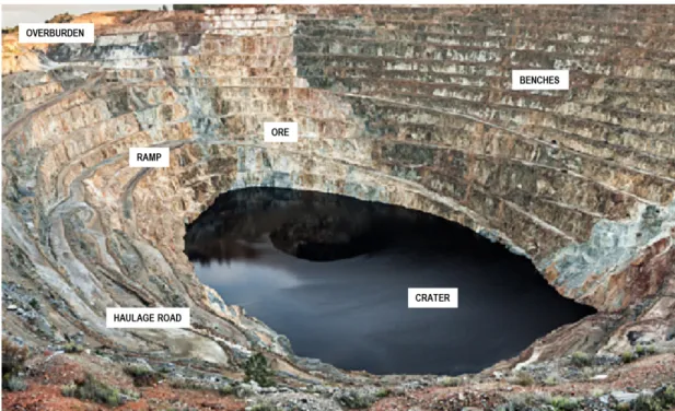
The mining of hard-rock mineral deposits occurs either via surface mining meth-ods, underground methods or a combination thereof. An open pit mine utilises a surface mining method, which is suitable when ore material is close to the surface of the earth. This method of exploitation has been around for much longer com-pared to underground mining methods and is more productive. Surface mining methods include strip mining and open-pit mining and is a broad category of mining in which soil and rock overlying and waste interspersed with the mineral deposit are removed (see Figure 2.1). In comparison, in an underground mine the overlying rock is left in place, and the material of interest is removed through

shafts or tunnels.

Figure 2.1: Open pit mine

In order to commence mining of valuable mineralised material (ore), large amounts of overburden (waste) must often be removed. This might include both unconsolidated material, removed relatively easily (and inexpensively), or harder material that requires drilling and blasting with explosives.

2.2.2

Mining activities

Surface mining operations typically employ the use of trucks and shovels.

Shovels (or excavators) are large mechanical diggers with various sized buck-ets, working at the exposed faces (called benches) in the open pit.

In the most conventional configuration, haul trucks transport ore and waste from the bottom of the open pit to the surface where it is dumped as waste or stockpiled for later treatment as ore. Material to be processed immediately is deposited into large crushers which reduce the blasted fragments to more man-ageable sizes. Other forms of transport from the pit to the processing facility might include conveyor belts or piping.

Ore is further processed in a treatment (or processing) plant by means of physical or chemical processes which separate the valuable material from waste or tailings to produce a liberated or concentrated product. This product might be

sold as it is or undergo further processing (e.g. smelting, refining, beneficiation) before it is sold to consumers in the market.

2.3

Data collection and interpretation

The profitable extraction of mineralised ore and waste requires the development of a pit design (outline) and an extraction schedule for the operations. The de-velopment of an optimised design and mining schedule requires the effort of a number of role players and the collection, calculation, modification and compila-tion of a large amount of data. This process starts already during drilling and sampling of drill cores and compositional assay of samples by a qualified labo-ratory in order to obtain sample grades and densities. This information is then compiled into a database for use by the geologist to create a geological and grade model.

2.3.1

Drilling, sampling and geological modelling

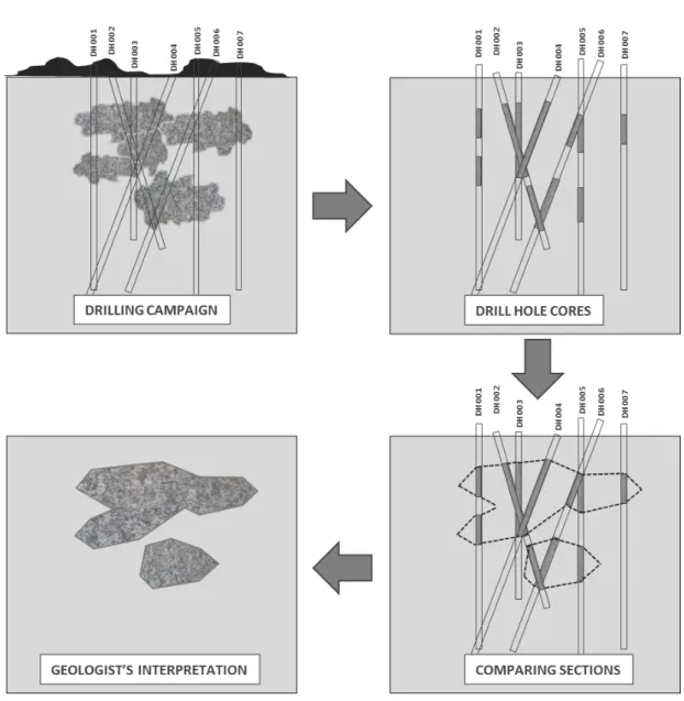
The process of converting information obtained from a series of drill holes into a block model is explained by Froyland et al. (2004). A number of long, narrow holes are drilled into the ore body (or where it is expected to be) and the cores are removed, logged and analysed (‘assayed’) for mineral concentrations and other material characteristics. Geologists use drill core logs and their location/spatial information to create a 3-D geological or lithological model by interpreting the spatial continuity of geological units - see Figure 2.2.

Important information obtained from such analyses are the material density and metal content or concentration (the grade) contained in the drill cores. Drill hole cores however only provide a sparse and limited set of data from which a full 3-D model of rock and metal characteristics needs to be constructed. Such a model construction is commonly done using geostatistical methods.

2.4

Geostatistics

Geostatistical estimation is a deterministic approach used in the generation of estimates for block values (e.g. metal grade) in the absence of perfect information. Various well known classic textbooks Journel and Huijbregts (1978), Clark (1979), Deutsch (2002) and guidelines are available that expand on the concepts, benefits and limitations relevant to geostatistics.

Figure 2.2: Geological interpretation from drill hole data

Whereas classical statistics hold that individual members of a population are positionally unrelated or random, in geostatistics a fundamental assumption is that individual members of a population within the mineralisation are positionally dependent and related. It is this dependence that enables the development of a mathematical model of a mineral deposit. This relationship is the basis of assumptions and predictions made of the size and grade of a mineral deposit.

A key geostatistical concept is that the values of samples located inside a block to be estimated are related to the value of the block and that the values of samples located closest to the block to be estimated are similarly related to the value of the block. Based on this assumption, a mathematical relationship

(function) can be developed between the values of the samples and the value of the block based on distance to the centre of the block. This mathematical relationship is represented as a graph called the ‘variogram’.

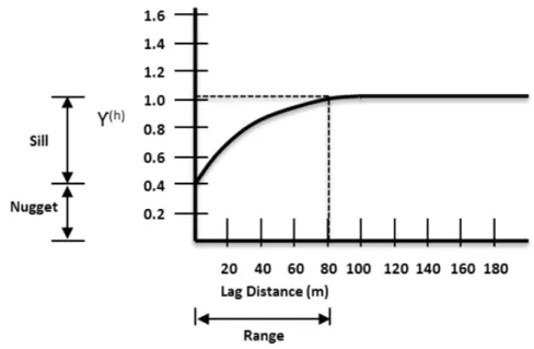
The (semi) variogram - There are numerous different types of variograms (relative variogram, semivariogram, log transformed variogram, etc.) The stan-dard spherical variogram is depicted in Figure 2.3.

Figure 2.3: Typical (idealised) Spherical Variogram

A number of basic concepts are relevant to the interpretation of the variogram: (a) the vertical axis represents the grade variability γ(h) between individual

points in the sample population.

(b) the Nugget represents the inherent (natural) variability of a sample - the result of inherent geologic variability or it could also be an ‘apparent’ effect due to sampling, sample preparation, and/or assaying error.

(c) the Sill indicates the point at which the variability between individual points in the sample population becomes uncorrelated.

(d) the Lag Distance (horizontal axis) is the average distance for grouping points for variogram calculation (i.e. minimum distance between sample points).

(e) the Range (shown on the horizontal axis in Figure 2.3) indicates the maxi-mum distance of influence which permits the correlation of values of samples and the value of the estimated block. At distances beyond the range, the mathematical relationship becomes random.

Kriging is a geostatistical estimation technique which has been commonly used for a number of decades. A number of different types of kriging variations are used depending on the circumstances (i.e. block kriging, point kriging, rankorder kriging, multiple-indicator kriging, etc.)

Kriging is believed to provide the best linear unbiased estimator of a point and the best linear weighted moving average of a block. Kriging minimizes the grade estimation variance when calculating the block grade from individual sample values. One of the well known limitation of block kriging is that it tends to over smooth the estimated values (Vann et al. (2002) and Journel and Huijbregts (1978)) resulting in estimated high-grade values that are less than the original sample values, and estimated low-grade values that are higher than the original sample values. By comparison, Conditional Simulation (explained later in this chapter) generates more representative values (see Figure 2.4).

Figure 2.4: Kriged vs. Conditionally Simulated models illustrating smoothing effect

2.4.1

Creating a block model

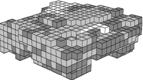
Mineralised ore bodies are modelled using a collection of blocks called a block model (see Figure 2.5). This type of model commonly consist of a three-dimensional accumulation of blocks which are characterized by their spatial location, weight and associated contained value (Journel and Huijbregts (1978) and Hustrulid and Kuchta (2006)).

Figure 2.5: Three-dimensional geologic block model representation of blocks (cubes) in a deposit

Block considerations - The regular three-dimensional fixed-block model is commonly used in block modelling since it is ideally suited to the application of computerised optimization techniques Gignac (1975). In addition to blocks being equally sized, the actual orthogonal dimensions of the blocks will be determined by a number of additional factors. These include:

(a) the physical characteristics of the mine - the orientation and dip of the deposit, structural features (faults, fractures, fold) which in turn influence safe pit slope requirements

(b) the variability of grade and metallurgical attributes - the more ‘massive’ the features the large the blocks, whereas intricate convoluted pockets of mineralisation require smaller block sizes in order to access the ore

(c) the size and capacity of mining equipment used - large scale mining equip-ment does not require small block sizes

The physical size and dimensions of blocks in a model and their effect on selectivity and value is discussed by Jara et al. (2006) and Hekmat et al. (2013) respectively.

Wharton (1996) cautions that decisions on block model size depend on the purpose of the modelling exercise. For instance this could be for (a) delineating the ore body, (b) for reserve value calculation, (c) for designing a pit or (d) for sensitivity analysis.

Block value - If a block contains sufficient valuable material compared to its total weight then the block can be classified as ore. A block that does not contain sufficient value to justify its extraction and processing expenses is classified as waste. Whether a block is classified as ore or waste will determine the profit (or loss) that the mining of a block might yield. However this decision is often not a straightforward decision and dependant on many factors.

The decision on whether a block should be classified as ore or waste is typically determine by the ‘cut off grade’.

According to Rendu (2008) the cut off grade is the minimum amount of va-luable product or metal that one metric ton (1000 kg) of material must contain before this material is considered for processing (and therefore extraction of the valuable product).

The direct profit or loss (or utility) Udir(x) expected from processing one

metric ton of material of grade x isUore(x), which is expressed as follows:

Uore(x) = x·r·(V −R)−(M +P +O) (2.1)

where:

• x is the average grade of valuable product contained in a metric ton of material (also called the ‘ore’)

• r is the metal recovery, or proportion of valuable product recovered from a metric ton of mined material

• V is the value of one unit of recovered valuable product (the ‘grade’) con-tained in a metric ton of material

• M is the mining cost incurred in mining a metric ton of material

• O is the overhead cost cost incurred in mining and processing a metric ton of material

• Ris the refining, transportation and other costs incurred per unit of valuable product contained in a metric ton of material

In order for values to be attributed to individual blocks, a number of techno-economic factors need to be decided. These include:

(a) Commodity price forecast for the metal(s) for which value needs to be as-signed. These could be static prices which remain constant over the schedul-ing period or period specific prices if that level of detail is available or required.

(b) Mining operating costs associated with e.g. drilling and blasting, dig-ging/excavation, hauling, primary crushing.

(c) Processing or treatment operating costs associated e.g. secondary (or ter-tiary) crushing, leaching, floatation, de-watering, concentration, comminu-tion etc.

(d) Metal recovery% related to different types of rock and their interaction with mining and processing equipment and processes.

(e) Discount factor, which is related to the deteriorating effect of time on value. Blocks scheduled for mining later will be more severely discounted (‘pe-nalised’) than blocks mined earlier. A decision on the discount rate (which determines the discount factor) is important and is a function of the com-pany’s funding regime (lending, equity or owner’s capital) plus a risk pre-mium.

(f) Capital expenditure (CAPEX) associated with the mining and processing equipment and facilities. CAPEX is often excluded from a schedule opti-misation unless the objective requires the resolution of variables associated to capacity levels and their associated CAPEX.

When the point is reached where a block model is developed with spatial locations (x,y,z coordinates), block dimensions (block size in the x,y,z directions) and key attributes such as block density (or tonnage), metal grade, ore/waste classification and recovery then further economic evaluation and analysis can be performed.

Economic Evaluation - Accumulating the values of these blocks over a time horizon together with the capital expenditure required to provide production and processing capacity to the process enables the derivation of a discounted cash flow (DCF) and net present value (NPV). The ultimate objective of any mining evaluation is typically to maximizing the NPV of mined material and processed ore given a certain set of assumptions (e.g. prices, costs, capital expenditure).

A number of factors need to be understood and taken into account during the planning of the open-pit operation to determine the shape and size of an open-pit. Some of these factors include according to Armstrong (1990):

(a) geology, lithology, topography, property boundaries (b) extent of the deposit, localisation of mineralisation

(c) mining method, mining rate, processing rate, bench height (d) cut off grade, pit slopes

(e) material and metallurgical characteristics, ore recovery (f) mining and processing costs

Some of these considerations can be seen illustrated in Figure 2.6. For exam-ple, the bench height, which is the vertical distance between each horizontal level of the pit, should be set as high as possible within the limits of the size and type of equipment selected for the desired production.

The pit slope is one of the major factors that determines the amount of waste to be removed so as to mine the ore. The spatial location of blocks is important since blocks on lower levels of the pit cannot be accessed until those blocks above it have been removed in order to maintain the integrity of pit slopes. Remov-ing of blocks should therefore honour certain spatial requirements (precedence constraints).

The two examples show these aspects for two different types of deposit. The one on the left has a tabular sub-vertical orientation, whereas the one on the right has a more lensoidal and disseminated nature.

Figure 2.6: Example open pit configurations for two general types of deposit

At the end of the modelling process, mine planners have to decide whether, and if so when, blocks in a block model should be extracted and which blocks need to be discarded or sent to the treatment plant for further processing as ore. This is done through mine planning and scheduling.

For more explanations of mining terms, see Hustrulid and Kuchta (2006).

2.5

Geological and Mining Uncertainty

In the mining industry, decisions linked to millions and even billions of dollars are made based on limited information both from the point of view of our un-derstanding of the deposit which we hope to excavate profitably, and our ability to forecast future prices, costs and economic trends that will materialise only as time passes. Despite this lack of information, most mining companies still stick to traditional deterministic decision making methods. Fortunately over that last few years, probabilistic modelling approaches such as Conditional Simulation which take account of risks and uncertainties has seen an increase in their application.

Before defining Conditional Simulation it is worth looking at some general sources of risk and uncertainty in mining.

2.5.1

General Sources of Mining Risk

Mining projects are invariably designed on the basis of highly uncertain variables arising due to the inherent nature of the variables as well as the prohibitive cost of improving the level of knowledge. Variables related to geological, metal content and material characteristics are quantified based on sparse drilling and sampling data. Dowd and Pardo-Iguzquiza (2002) notes that since such programmes typi-cally provide data on a relatively large (regional) scale, the levels of resolution is understandably at an order of magnitude greater than the scale required for mod-elling, prediction and risk assessment. Key sources of mining risk and uncertainty are:

(a) Geological Uncertainty - the availability of drilling and sampling data in mining projects and operating mines are generally limited. This intro-duces a high level of geological uncertainty around the qualitative (what does it contain?), quantitative (how much does it contain?) and positional (where is it located?) characteristics of mineral deposits. These charac-teristics include the physical extent of the deposit, location of geological boundaries and contacts, geo-technical features (e.g. faults, fractures and folds) and geo-metallurgical properties (e.g. material density and metal recovery). Dunham and Vann (2007) expand on the importance of includ-ing geo-metallurgical uncertainty around issues such as characterisation of metallurgical recovery and throughput.

(b) Financial and Revenue factors - another major contributing factor to the total uncertainty of a mining project is the commodity price and ex-change rates. Depending on the type of commodity these are typically also highly uncertain. Metal prices are influenced by many contributing factors associated with supply (other producers) and demand (consumers). Prices are further influenced depending on whether commodities are sold based on long term contracts or spot market prices, seasonality in demand, level of substitution, demographical growth etc.

(c) Operating Costs - mining and processing operating costs (OPEX) are also uncertain since they are associated with unpredictability in seasonal and growth trends of inflation rates, as well as availability and cost (supply and demand) of key production factors such as labour, tyres and power). (d) Capital Expenditure due to the complexity of the cost estimation

pro-cess, as well as the long duration between the time of estimation and the time of expenditure, capital expenditure (CAPEX) is similarly uncertain. (e) Efficiency and Performance factors - factors such as metal recovery,

dilution, production and processing efficiency are uncertain since they are either tied to geological uncertainty or related to future performance of human resources and equipment.

(f) Other- more subjective risks such as political, country related, social and environmental is difficult to quantify and often ends up in some form built into the project specific discount rate as a risk premium.

The combined effect of all these levels of uncertainty is that geologists and mining engineers have a difficult time compiling evaluations and business cases for mineral projects. Typically, uncertainty in estimation and forecasting is pro-hibitive on the accuracy of assumptions made in feasibility studies. This fact is evident from confidence intervals that decision makers typically put around different levels of study. Research conducted by Hall (2007) proposes confidence intervals for various types of studies from around 30% for conceptual studies, typically 20-25% for pre-feasibility studies and 10-15% for feasibility studies. In addition to these confidence intervals, Bullock (2011) indicates that a range of contingencies are also typically added to the bottom-line expected cost of the estimate depending on the level of accuracy.

Arguably the two most important areas of uncertainty influencing the ac-curacy and validity of mining case studies are those associated with geological (grade) and price uncertainty.

Within this thesis we only focus on the quantification of grade uncertainty but a lot of work has been done on various ways to incorporate price uncertainty into the mine planning and scheduling process. Some of the key methods used are Monte Carlo Simulation and Real Option Valuation.

Literature Review

3.1

Introduction

This chapter reviews key literature relevant to the Open Pit Production Schedul-ing Problem. It starts off by lookSchedul-ing at research related to deterministic method-ologies and then follows with a review of research which introduces grade uncer-tainty into the optimisation problem via probabilistic and stochastic modelling.

The next section (Section 3.2) considers the most relevant modelling and optimisation methods (deterministic) and related literature. This is divided firstly into Sequential Approaches (Section 3.2.1), which break the problem up into ultimate pit optimisation, push back generation and then scheduling. We then secondly consider Integrated Approaches (Section 3.2.2) which solve the problem as a whole.

In Section 3.3 we introduce risks related to mining with a focus in Section 3.3.3 on the use of Conditional Simulation methods. Section 3.3.4 discusses various Stochastic approaches and Section 3.3.5 covers Scenario Optimisation approaches.

3.2

Deterministic Mine Planning and

Schedul-ing Methodologies

A strategic solution to the open pit production scheduling problem involves de-cisions pertaining to:

(a) which of the available blocks in a mining block model to extract (i.e. mine them or leave them in the ground),

(c) what to do with the extracted material (send mined block to waste, to the processing plant for treatment or to a stockpile for later consideration). Open pit mining production scheduling has been traditionally approached via two different angles. In the one case (the more traditional approach) the develop-ment progresses sequentially through three stages starting with the determination of the ultimate pit limits, followed by the development of a number of push backs or mining pits. This is then followed by the solution of optimised schedules for each push back. This is called the Sequential Approach in this thesis.

The other approach, called the Integrated Approach here, takes a holistic view of the problem to determine the optimal block extraction sequence, avoid-ing sub-optimal mine schedules that are inherently created usavoid-ing the sequential approach.

3.2.1

Sequential modelling approach

During the Sequential Approach, the mine design and schedule is generated in three distinct stages.

(a) Firstly, Ultimate Pit Limits are determined by applying an expected com-modity price to the model and solving essentially a single period (i.e. no discounting) optimisation. This step requires that the cut off grade (the grade separating ore from waste) is fixed.

(b) In a second step, the blocks contained in the Ultimate Pit is subjected to a parametrisation procedure which generates a set of Nested Pits each corresponding to different price or revenue factors. Nested pit shell are then grouped together in such a way as to generate a limited number of Push Backs which allow reasonable ore to waste ratios see Figure 3.2.

(c) In a final step the blocks in each push back or grouping is solved separately as a Schedule allowing the sequencing of blocks in time.

Generating the Ultimate Pit

The Ultimate Pit is the design outline which delimits the extremities of the ma-terial targeted for mining (or the optimal boundary). The set of blocks contained within this design maximises the total profit of the pit so that adding or removing any blocks from this design will lead to a loss in value. The problem of finding

the set of blocks that should be removed in order to maximise the total profit from a mine, subject to the constraints on pit slopes, is known as theUltimate Pit Limit Problem (UPLP).

Over the years, various types of methods have been employed to solve the UPLP. These include Graph Theory and Network Flow algorithms, Dynamic Pro-gramming, heuristics such as the Moving (Floating) Cone method, parametrizing functions and exact optimization approaches such as Linear Programming.

A large volume of literature is available on the solution to the UPLP. Overviews of various vintages on the applicable literature are provided by Kim (1979), Kim et al. (1988), Laurich and Kennedy (1990), Dincer and Golosinski (1993), Dagde-len (2001) and Newman et al. (2010). Traditionally the UPLP has most often been solved using versions and modifications to Lerchs and Grossmann’s Graph Theory algorithm (Lerchs and Grossmann, 1964) or by solving Picard’s Network Flow formulation (Picard, 1976).

Graph Theory was applied by Lerchs and Grossmann (1964) to model an open pit mine as a weighted, directed graph. In the same paper they also used dynamic programming to solve two-dimensional versions of the UPLP. In this model where vertices represent blocks and arcs represent mining restrictions (i.e. sequencing constraints) ultimate pit limits are determined by solving for the max-imum closure of this graph. The problem of generating optimal mine schedules was raised and researched by Johnson (1968) who developed an LP formulation for optimising the timing of extraction of regularised resource blocks within a mine, with a maximum NPV objective. Johnson and Sharp (1971) presented a three-dimensional dynamic programing method for determining the optimal ultimate open pit limit which is an extension of the two-dimensional Lerchs-Grossmann ap-proach. Koenigsberg (1982) reviews the state of the art of dynamic programming and demonstrates the connection between linear programming (and network flow) models and the dynamic programming method. Caccetta and Giannini (1988) build on the graph-theoretic approach of Lerchs and Grossman through the use of a dynamic programming technique to ‘bound’ the optimum. A similar approach to Lerchs and Grossman with some modifications has been employed by Zhao and Kim (1992) in which they claim to solve problem instances faster than the method proposed by Lerchs and Grossman. Huttagosol and Cameron (1992) ex-tended the optimizing model based on the maximum closure of a graph developed by Lerchs and Grossmann for solving ultimate pit limit problems. Yegulalp and

Arias (1992) builds on the work of Johnson and Barnes (1988) to offer a modifi-cation of the push-relabel maximum flow problem (the excess-scaling algorithm). They show however that Whittle Programming Pty. Ltd.’s implementation of the Lerchs and Grossman algorithm has faster computation times than their own implementations of the excess-scaling algorithm. Seymour (1995) proposes a modified 3D Lerchs-Grossmann graph tree algorithm that generates a complete set of nested maximum valued pits in a single run. Underwood and Tolwinski (1998) build on the work of Lerchs and Grossman by developing a network flow algorithm based on the dual formulation to solve the same problem. Their results adds insight to the LG algorithm and provides proposals for efficiency improve-ments. Hochbaum and Chen (2000) makes a detailed comparison between the LG algorithm and the maximum flow ‘push-relabel’ algorithm and proposes an efficient implementation of the push-relabel algorithm adapted to the features of the open-pit mining problem. Askari-Nasab and Awuah-Offei (2009) explores the validity of a theorem that a pit outline determined by an optimal long term schedule algorithm is constrained by the conventional Lerchs and Grossmann’s optimised pit outline. This hypothesis was investigated through a case study using an intelligent open pit simulator founded on agent based learning theories. Despite the fact that the Lerchs-Grossmann algorithm provided an important tool for mine design over the years, its use for scheduling is restricted to mines having a very short life (up to 3 years) as time is not an input parameter (Cac-cetta and Hill, 2003).

Network flow algorithms have been used to model the ore body as a di-rected node-weighted graph which is associated with the 3-dimensional block model. A network of nodes represents the blocks in the mine, connected by arcs which represent the sequencing constraints between the blocks. The net-work model of the ore body is constructed by addition of two nodes to its graph model: a source node and a sink node. Arcs are then generated from the source to all positive nodes, and from all negative nodes of the graph to the sink. The goal of such a model is to maximize the flow from a source node to a sink node. Arcs originating at the source which have excess capacity upon termination of the algorithm indicate to profitable blocks that should be mined in the optimal solution. Such profitable blocks together with any blocks required to be mined to reach them represent the ultimate pit limits.

Network flow algorithms have been utilised by Picard (1976), Caccetta and Giannini (1988), Giannini et al. (1991), Yegulalp and Arias (1992) and Hochbaum

and Chen (2000) to derive solutions for the ultimate pit limits problem.

In the Dynamic Programmingapproach, the UPLP is usually decomposed into smaller sub-problems and most favourable decisions for the sub-problems are to be made at each stage. Namely, the decisions are optimised at subsequent stages rather than simultaneously. With this approach a trade off is made between the desire to obtain the highest possible value at the present stage against the implication this would have on value at future stages (Saavedra Rosas, 2009).

Dynamic programming methods have been used to solve two-dimensional sions of the UPLP (Lerchs and Grossmann, 1964) while three-dimensional ver-sions of the problem are solved by Koenigsberg (1982), Wilke and Wright (1984), Wright (1987), Caccetta and Giannini (1988), Sevim and Lei (1994) and Yam-atomi et al. (1996).

A number of heuristic methods have been used to solve the UPLP. One of the most well known is the Moving (Floating) Cone Method which has been widely used due to its simplicity. The Moving Cone Method assumes a block has a reference point for expanding the pit upward according to given pit slope rules. This upward expansion containing all blocks (whose removal is necessary for the removal of the reference block) forms a cone whose economic value can be determined. Early solutions using the Moving Cone Method were proposed by David et al. (1974), Lemieux (1979) and modifications were proposed by Yamatomi et al. (1996). A more recent variation of the floating cone algorithm called the floating stope method was developed for underground by Alford (Alford and Hall, 2009) but it fails to render optimal ultimate pit limits.

Approaches based on exact optimization are also common ways of solving the ultimate pit limits problem. Linear programming methods are used by Meyer (1969),Gershon (1982) and Huttagosol and Cameron (1992) to solve the ul-timate pit limits problem. Gershon (1983) identifies and discusses computational difficulties arising in the solution of linear programming models as a mitigation against their widespread use in mine scheduling. In particular he notes with respect to Johnson’s LP formulation that it mined partial blocks producing in-feasible solutions as sequencing constraints are violated. Due to the fractional solution provided by the LP formulation, integer constraints are needed to pro-duce feasible solutions. While the MIP formulation is theoretically robust, the solution of large scale problems was not practical with the computer hardware of the 80’s and 90’s (Gershon, 1983) but this changed with the research of Caccetta and Hill (2003).

Creating push backs

Following the Sequential Approach, the optimization of open pit mine design consists primarily of defining the ultimate pit limits and then dividing up the pit into manageable volumes of material often referred to as push backs (also called cutbacks, or phases).

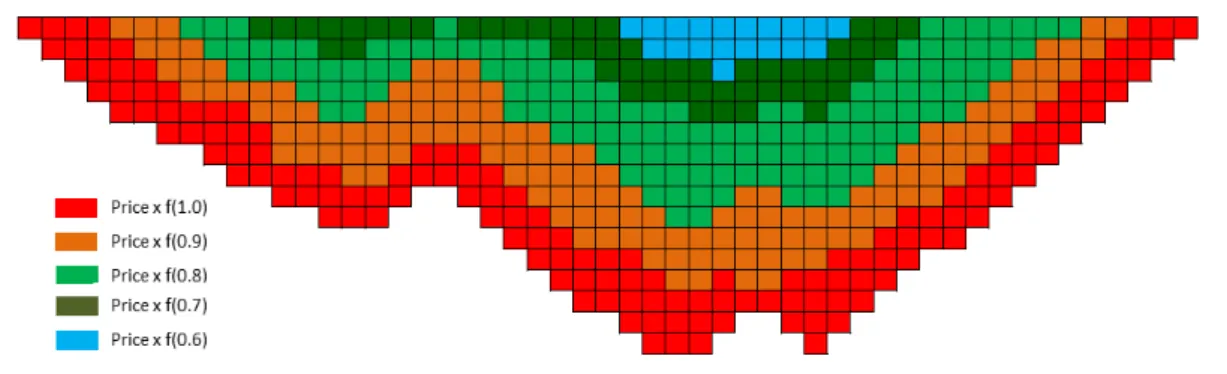
A popular technique for producing push backs is to utilise an algorithm that produces the ultimate pit and rerun it multiple times over the orebody model while the economic block values are scaled down (‘parametrized’) by a series of decreasing factors - e.g. see Figure 3.1 showing a length-wise section through the block model.

Figure 3.1: Nested pits illustrating parametrisation - section view length-wise through block model

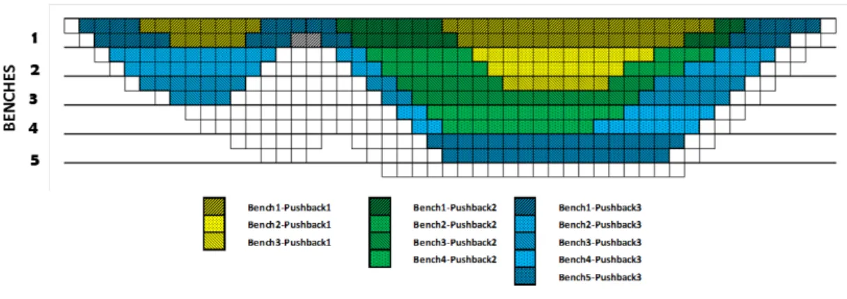
Push backs, allow the mine designer to develop short term schedules for a smaller more manageable sub-set of the blocks considered. They also contribute to the yearly production schedules so one can apply an economic discount rate when calculating the Net Present Value of the mine. Push backs are produced from the sections of the orebody model that remain within the ultimate pit limits. Push backs and benches are often combined to generate benchpush back units -see Figure 3.2.

Figure 3.2: Bench-push back units - section view length-wise through block model The concept of parametrization was introduced by Lerchs and Grossmann (1964) as a way to generate an extraction sequence. Using an undiscounted model, they proposed varying the economic value of each block by penalising it with an increasing factor. This leads to a set of nested pits which can be used to produce a production schedule. Dagdelen and Francois-Bongarcon (1982) present development of a double parameterization algorithm and Dagdelen and Johnson (1986) describe the fundamentals of a new algorithm based on lagrangian relax-ation and parameterizrelax-ation. Modificrelax-ations to the original work has also been proposed by Caccetta et al. (1998).

A number of authors have expanded on the theme of nested pit or push back generation. Mathieson (1982) discusses an overall mine planning methodology with emphasis on the design of an optimal sequence of pit expansions or phases. Kim and Zhao (1994) reviews methodologies for developing the pit sequence or staggered pit phases. Gu et al. (2010) presents a model in which a sequence of geologically optimum pits is first generated and then dynamically evaluated to simultaneously optimize the number of phases, the geometry and location of each phase-pit (including the ultimate pit), and the ore and waste quantities to be mined in each phase. The objective is to maximize the overall net present value.

Scheduling

As the final step in the Sequential Approach Optimised schedules are derived within and are bounded by the predetermined volumes defined as push backs. Traditional production scheduling methods are commonly performed using push backs designed to maximize the economic value, or metal content within each incremental push back in a greedy fashion.

Issues with the Sequential Approach

Some of the common issues with the Sequential Approach that lead to sub-optimal production schedules are:

(a) not considering requirements in grade and ore quality parameters; (b) inability to incorporate mining and processing capacity constraints;

(c) inability to incorporate blending targets in the calculation of the ultimate pit boundaries (Stone et al., 2007);

(d) ignoring the deposit grade uncertainty;

(e) unsuitability of the LG shells as a basis for mining phase design in more complex operations with:

• multi-dimensional blended ore targets,

• multiple products with market constraints,

• multiple processes with capacity constraints,

• sinking rate constraints

• exposed ore constraints

(f) large variations in size of the push backs, or the so-called ‘gap problem’ leading to impractical results;

(g) not considering discounting during the optimization;

(h) assuming that a greedy approach will maximize discounted value.

3.2.2

Integrated modelling approach

The second approach is comprehensive and attempts to solve the scheduling prob-lem in a single stage without preconceived assumptions about ultimate pit limits, push backs or stages.

A more integrated approach using mixed-integer linear programming (MILP), allows for the simultaneous definition of optimal mine production schedules within their ultimate pit limits without having to determine push back phases. MILP methods have been used for solving the mine production scheduling problem using a branch and cut strategy together with linear relaxation (Caccetta and Hill (2003), Bley et al. (2010)).

Current integrated production scheduling methods can be roughly divided into Heuristic methods and Exact methods.

Heuristic methods

Heuristic methods include Local Search algorithms such as Hill Climbing and Simulated Annealing, Tabu Search, Particle Swarm Optimization, Ant Colony Optimization and Genetic Algorithms.

Local Search algorithm paradigms aim to find an optimal solution for a problem by means of selecting the next potential solution from a set of neighbours of the current solution (hence the name local search). A general characteristic of local search algorithms is that it is ’memoryless’ meaning that decisions taken are not influenced by decisions taken in the past or future considerations.

The Hill-Climbing Algorithm is a variation on the local search heuristic theme. In this approach the decision to progress is governed by each successive solution considered being an improvement to the previous (i.e. lower cost or greater value). The algorithm can be ‘randomized’ if it selects prospective moves randomly from neighbours, or ‘greedy’ if it only selects from the best next moves. Hill-climbing methods often end up at local optima but benefit from simplic-ity and solution speed as favourable arguments especially when applied to large problems, as an approximation or for rapid exploration of the solution space.

The Metropolis and Simulated Annealing algorithms are modifications on the theme of hill-climbing algorithms. They employ a probabilistic scaling on improvements similar to a temperature parameter. Simulated Annealing allows for varying temperature.

Yun et al. (2005) briefly covers the so-called field of ‘computation intelligence’ citing the use of genetic algorithms, genetic programming, evolutionary program-ming, artificial neural networks and ant colony algorithms as recent applications in solving mining problems.

Amaya et al. (2009) describe a scalable IP-based methodology for solving very large (millions of blocks) instances of this problem by embedding standard IP technologies in a local-search based algorithm they obtain near-optimal solutions to large problems in reasonable time.

In the Tabu-Search Algorithmthe local search algorithm contains a mech-anism which tries to avoid certain possible loops captured on a tabu list aiming to provide a type of memory regarding recently visited unfavourable states not to be chosen during future state updates. Lamghari and Dimitrakopoulos (2012)