i
Performance Analysis of IPv4 vs. IPv6 on various
Operating Systems using Jumbo Frames
Name: Paula Raymond Lutui
A thesis submitted in partial fulfilment of the requirements for the
degree of Master of Computing
ii
Abstract
The services offered on the Internet, the requirements and demands for use of multimedia applications, such as sharing video files, photos, video conferencing, and the increased usage of social networking sites, have all contributed to the exponential growth of the Internet usage over the last ten years. In order to meet these demands, hardware developers have increased the speed of hardware such as processors and switches, and routers, also have increased capacity of the communication medium. However, the maximum data unit that can be passed onwards by any layer via this communication medium remains untouched. The current Maximum Transfer Unit (MTU) is 1500 Bytes, to address this issue, a new MTU has been emerged which is known as Jumbo frames. The proposed MTU for Jumbo frames in now 9000 Bytes.
The purpose of this study is to evaluate the performance of Jumbo frames on a network environment employing six operating systems from two different distributions. These operating systems are; Microsoft Windows Server 2008, Microsoft Windows Server 2003 and Microsoft Windows 7 Professional and from the Linux distributions, Linux Fedora, Ubuntu and OpenSUSE. In this study, two transmission protocols were employed namely, Transmission Control Protocol (TCP) and the User Datagram Protocol (UDP). Two Internet protocols were also engaged in these performance experiments, Internet Protocol version six (IPv6) and Internet Protocol version four (IPv4). There were five main performance metrics extracted from the data collected in this experimental study namely the throughput, delay, jitter, the CPU utilisations on the software routers and the packets dropped rate. The experiments were conducted on the network level and at the application level with the following applications; DNS, Games and VoIP traffics on five different VoIP CODECs. The Jumbo frame sizes involved ranging from 1518 Bytes to 9014 Bytes.
The findings of this study concluded that for traffic employing TCP as transport protocol, Microsoft Windows Server 2008 and Microsoft Windows 7 yielded the highest throughput on both IPv6 and IPv4 and also Linux OpenSUSE on IPv4 only. When UDP was employed as transmission protocol, all of the operating systems yielded similar throughput values
With regards to the applications‟ results, the findings of this study concluded that for DNS, Microsoft Windows Server 2008 and Microsoft Windows Server 2003 yielded the highest throughput on IPv6 and Linux Fedora on IPv4. For the games on IPv6, Linux Ubuntu yielded the highest throughput on the CSa game while all of the operating systems yielded similar values on the CSi game. On the Quake3 game, Microsoft Windows Server 2008 produced the highest throughput values.
iii With regards to the VoIP on IPv6, Microsoft Windows Server 2003 and Linux Ubuntu yielded the highest throughput on the G.711.1 CODEC while OpenSUSE yielded the highest values on the G.711.2 CODEC hence; Microsoft Windows Server 2008 generated the highest amount of delay on all of the CODECs. With regards to VoIP on IPv4, Microsoft Windows 7 yielded the highest throughput on the G.711.1 CODEC while Microsoft Windows 7, Linux Fedora and OpenSUSE yielded the highest values on the G.711.2 CODEC however, on both IPv6 and IPv4 for the G.723.1, G.729.2 and the G.729.3 CODECs, all of the operating systems yielded similar throughput values. The good combination for IPv6 on VoIP would be Microsoft Windows Server 2003 or Linux Ubuntu on the G.711.1 CODEC, they both yielded high throughput but low delay and low jitter and for IPv4, Microsoft Windows 7 on the G.711.1 or G.711.2 CODECs; it yielded high throughput but low delay and low jitter.
iv
Acknowledgement
It is such an amazing feeling to complete this study for my thesis however; I have a sense of duty to acknowledge the guidance and support I received from all the experts who assisted me in the compilation and successful completion of this paper.
Firstly, I would like to give thanks to the King of kings and the Lord of lords for giving me the most precious gift of all, which is the gift of life and for allowing me to effectively complete this work.
Secondly, I would like to thank my principal supervisor Shaneel Narayan who has been with me from the very beginning right through to the completion of this study. He was always there when I needed him; he listened and provided advice and ideas on how to tackle the technical problems I encountered. I would also like to thank my associate supervisor Aaron Chen for his assistance during the compilation of this document.
Thirdly, I would also like to acknowledge the privilege I had during this research to work together with Professor Dr. Kay Fielden. Her guidance and expert advice during the compilation of this document was priceless.
Last but not least, I want to acknowledge the help and support I receive from my family. They have been my silent partner during this work. The prayers, the encouragement and the support not only during this work but throughout my Master of Computing study, were the motivating force I needed during this journey and to them I am forever grateful.
v
Table of Contents
Abstract ... ii Acknowledgement ... iv List of Tables ... ix List of Figures ... xList of Abbreviations ... xiii
Publications ... 1
Chapter 1: Introduction ... 2
1.1 Structure of the Report ... 4
Chapter 2: Literature Review ... 5
2.1 Literature Background ... 5
2.1.1 Networking and Network Performance. ... 5
2.1.2 Performance Analysis ... 7
2.2 Internet Protocol ... 11
2.3 The Transmission Protocols ... 17
2.4 The Network Performance Measurement Tools ... 19
2.4.1 IP Traffic ... 20
2.4.2 Iperf ... 21
2.4.3 Netperf ... 22
2.4.4 Multi-Generator (MGEN) ... 22
2.4.5 Distributed Internet Traffic Generator (D-ITG) ... 23
2.5 Performance Measurement Tool for this Study ... 23
2.6 Jumbo Frames ... 25 2.7 Literature Analysis ... 28 2.9 Chapter Summary ... 29 3.0 Methodology ... 30 3.1 Hypotheses ... 30 3.2 Research Methods ... 31
3.3 Methodology Employed for this Study ... 34
3.4 Data Collection Method ... 34
vi
4.0 Experimental Setup ... 38
4.1 Hardware Specifications ... 38
4.2 Software Specifications ... 39
4.3 Network Design ... 39
4.4 Determining the Optimal Value ... 40
4.5 Optimal Values for this Study ... 45
4.6 Chapter Summary ... 46
Chapter 5: Data Analysis ... 47
5.1 TCP Analysis ... 47
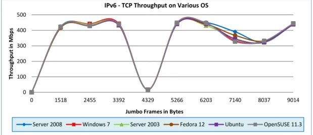
5.1.1 TCP Throughputs on IPv6 & IPv4 Jumbo Frames ... 47
5.1.2 Compare TCP Throughputs on IPv4 & IPv6 Jumbo Frames ... 49
5.1.3 TCP One Way Delay on IPv6& IPv4Jumbo Frame ... 50
5.1.4 Compare TCP Delays on IPv4 & IPv6 Jumbo Frames ... 52
5.1.5 TCP Jitter on IPv6 & IPv4 Jumbo Frame ... 53
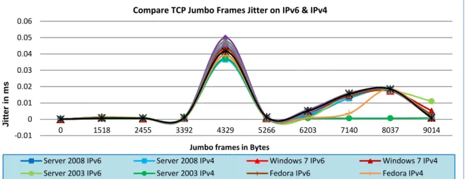
5.1.6 Compare TCP Jitter on IPv4 & IPv6 Jumbo Frames ... 54
5.1.7 TCP CPU Utilisations for Router 1 on IPv6 & IPv4 Jumbo Frame ... 55
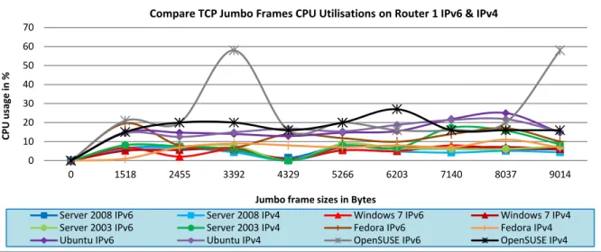
5.1.8 Comparing TCP CPU Utilisations for Router 1 on IPv4 & IPv6 Jumbo Frames. ... 57
5.1.9 TCP CPU Utilisations for Router 2 on IPv6 & IPv4 Jumbo Frame ... 58
5.1.10 Comparing TCP CPU Utilisations for Router 2 on IPv4 & IPv6 Jumbo Frames. ... 60
5.2 UDP Analysis ... 61
5.2.1 UDP Throughput on IPv6 & IPv4 Jumbo Frames ... 61
5.2.2 Compare UDP Throughputs on IPv4 & IPv6 Jumbo Frames ... 63
5.2.3 UDP One Way Delay on IPv6 & IPv4 Jumbo Frame ... 64
5.2.4 Compare UDP One Way Delay on IPv4 & IPv6 Jumbo Frames ... 66
5.2.5 UDP Jitter Results on IPv6 & IPv4 Jumbo Frame ... 68
5.2.6 Compare UDP Jitter Results on IPv4 & IPv6 Jumbo Frames ... 70
5.2.7 UDP Packets Dropped on IPv6 & IPv4 Jumbo Frame ... 71
5.2.8 Compare Packets Dropped Results on IPv4 & IPv6 Jumbo Frames ... 73
5.2.9 UDP CPU Utilisations on IPv6 & IPv4 Jumbo Frame on Router 1 ... 75
5.2.10 Compare UDP CPU Usage for Router 1 on IPv4 & IPv6 Jumbo Frames ... 77
5.2.11 UDP CPU Utilisations on IPv6 & IPv4 Jumbo Frame on Router 2 ... 79
vii
5.2.13 Compare TCP & UDP Throughput on IPv6 Jumbo Frames ... 82
5.2.14 Compare TCP & UDP Throughput on IPv4 Jumbo Frames ... 85
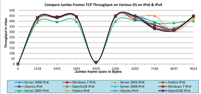
5.2.15 Compare Jumbo Frames IPv6 & IPv4 Throughput on TCP ... 87
5.3 Applications Analysis ... 90
5.3.1 DNS Throughputs on IPv6 & IPv4 Jumbo Frames ... 90
5.3.2 Compare DNS IPv6 & IPv4 Throughput results on Jumbo Frames ... 91
5.3.3 DNS Delay in IPv6 & IPv4 Jumbo Frames ... 92
5.3.4 Compare DNS IPv6 & IPv4 Delay results on Jumbo Frames ... 93
5.3.5 DNS Jitter on IPv6 & IPv4 Jumbo Frames ... 94
5.3.6 Compare DNS IPv6 & IPv4 Jitter results on Jumbo Frames ... 95
5.3.7 DNS CPU Usage on Router 1 on IPv6 & IPv4 Jumbo Frames ... 96
5.3.8 Compare DNS IPv6 & IPv4 Usage results on Router 1 on Jumbo Frames ... 97
5.3.9 DNS CPU Usage on Router 2 on IPv6 & IPv4 Jumbo Frames ... 98
5.3.10 Compare DNS IPv6 & IPv4 CPU Usages on Router 2 on Jumbo Frames ... 99
5.3.11 Games Throughput Results on IPv6 & IPv4 Jumbo Frames ... 100
5.3.12 Compare Games Throughput Results on IPv6 & IPv4 Jumbo Frames ... 101
5.3.13 Games Delay Results on IPv6 & IPv4 Jumbo Frames ... 103
5.3.14 Compare Games Delay Results on IPv6 & IPv4 Jumbo Frames ... 105
5.3.15 Games Jitter Results on IPv6 & IPv4 Jumbo Frames ... 106
5.3.16 Compare Games Jitter Results on IPv6 & IPv4 Jumbo Frames ... 108
5.3.17 Games CPU utilisations Results on Router 1 IPv6 & IPv4 Jumbo Frames ... 110
5.3.18 Compare Games CPU Usage Results on IPv6 & IPv4 Jumbo Frames on Router 1 .. 112
5.3.19 Games CPU utilisations Results on Router 2 IPv6 & IPv4 Jumbo Frames ... 115
5.3.20 Compare Games CPU Usage Results on IPv6 & IPv4 Jumbo Frames on Router 2 .. 117
5.3.21 Games Packets Dropped Results for IPv6 & IPv4 Jumbo Frames ... 119
5.3.22 Compare Games Packets Dropped Results on IPv6 & IPv4 Jumbo Frames ... 121
5.3.23 VoIP Throughput Results for IPv6 & IPv4 Jumbo Frames ... 123
5.3.24 Compare VoIP Throughput Results on IPv6 & IPv4 Jumbo Frames ... 126
5.3.25 VoIP Delay Results for IPv6 & IPv4 Jumbo Frames ... 128
5.3.26 Compare VoIP Delay Results on IPv6 & IPv4 Jumbo Frames ... 130
5.3.27 VoIP Jitter Results for IPv6 & IPv4 Jumbo Frames ... 132
viii
5.3.29 VoIP CPU Usage Results for IPv6 & IPv4 Jumbo Frames on Router 1 ... 136
5.3.30 Compare VoIP IPv6 & IPv4 Jumbo Frames CPU Usage Results on Router1 ... 138
5.3.31 VoIP CPU Usage Results for IPv6 & IPv4 Jumbo Frames on Router 2 ... 139
5.3.32 Compare VoIP IPv6 & IPv4 Jumbo Frames CPU Usage Results on Router2 ... 142
5.3.33 VoIP Packets Dropped Results for IPv6 & IPv4 Jumbo Frames on Router2... 143
5.3.34 Compare VoIP Packets Dropped Results on IPv6 & IPv4 Jumbo Frames ... 145
5.4 Summary ... 147
Chapter 6: Discussion ... 148
6.1 TCP Performance on Jumbo Frames with IPv6 and IPv4 ... 148
6.2 UDP Performance on Jumbo Frames IPv6 and IPv4 ... 154
6.3 Comparison of TCP and UDP Performance on Jumbo Frames IPv6 and IPv4 ... 160
6.4 Applications Performance on Jumbo Frames IPv6 and IPv4 ... 162
6.4.1 DNS Performance on Jumbo Frames IPv6 and IPv4 ... 162
6.4.2 Games Performance on Jumbo Frames IPv6 and IPv4 ... 163
6.4.3 VoIP Performance on Jumbo Frames IPv6 and IPv4 ... 165
6.5 Summary of Discussions ... 167
6.5.1 Summary of Applications‟ Discussions ... 170
7.0 Conclusions ... 174
7.1 Further Study... 180
ix
List of Tables
Table 1.1: World Internet Users and Population Statistics ... 2
Table 2.1: Throughput measures and units used. ... 8
Table 2.2: IPv4 three main classes ... 11
Table 2-3: IPv4 header field and its corresponding IPv6 header field. ... 15
Table 2-4: Comparing the main differences of IPv4 and IPv6. ... 16
Table 2-5: Comparing TCP and UDP ... 18
Table 2-6: Computer specifications and operating systems employed. ... 27
Table 3-1: Features of Qualitative & Quantitative Research ... 33
Table 4-1: Hardware specifications ... 38
x
List of Figures
Figure 2-1: The TCP/IP model. ... 18
Figure 2.2: IP Traffic test and measure sample network... 20
Figure 2-3: D-ITG software architecture ... 23
Figure 2-4: Comparative study of traffic generators... 24
Figure 2-5: Throughput comparison using various tools ... 25
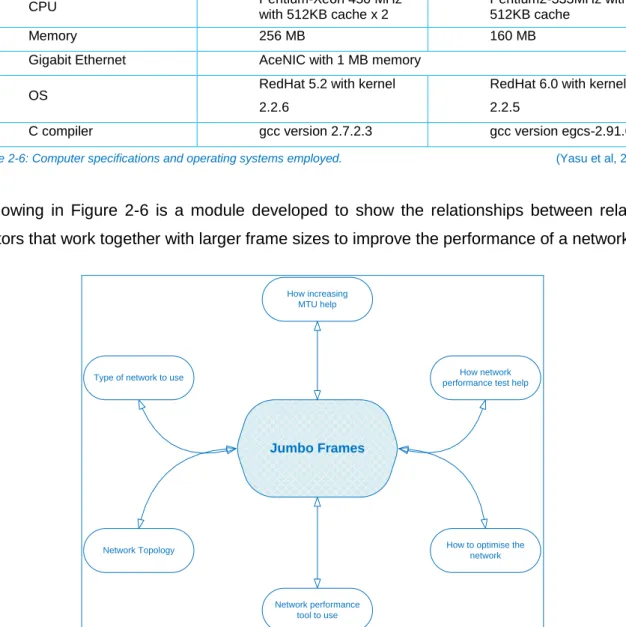
Figure 2-6: Jumbo frames module ... 27
Figure 3-1: Type of Research, Data Collection & Techniques. ... 31
Figure 3-2: Epistemological Assumptions for Qualitative & Quantitative Research. ... 33
Figure 3-3: Script used by ITGSend to generate traffics during the experiments. ... 35
Figure 3-4: Sample taken from data decoded by ITGDec. ... 36
Figure 3-5: Line graph example. ... 36
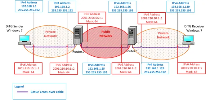
Figure 4-1: Diagram of network environment for this study. ... 40
Figure 4-2: TCP results on Microsoft Windows Server 2008 for packet size 3224 Bytes. ... 41
Figure 4-3: 6448 Bytes results. ... 41
Figure 4-4: 9672 Bytes results. ... 41
Figure 4-5: 12896 Bytes results. ... 42
Figure 4-6: 16120 Bytes results. ... 42
Figure 4-7: Differences in throughput between packet sizes 3224-6448 Bytes. ... 42
Figure 4-8: Differences in throughput between packet sizes 6448-9672 Bytes. ... 42
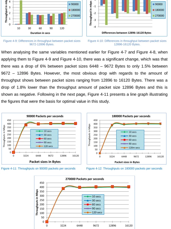
Figure 4-9: Differences in throughput between packet sizes 9672-12896 Bytes. ... 43
Figure 4-10: Differences in throughput between packet sizes 12896-16120 Bytes. ... 43
Figure 4-11: Throughputs on 90000 packets per seconds ... 43
Figure 4-12: Throughputs on 180000 packets per seconds ... 43
Figure 4-13: Throughputs on 270000 packets per seconds ... 43
Figure 4-14: UDP Throughputs on 3224 Bytes Packet size. ... 44
Figure 4-15: UDP Throughputs on 6448 Bytes Packet size. ... 44
Figure 4-16: UDP Throughputs on 9672 Bytes packet size. ... 44
Figure 4-17: UDP Throughputs on 12896 Bytes Packet size. ... 44
Figure 4-18: UDP throughput on 16120 Bytes Packet size ... 44
Figure 5-1-1: TCP IPv6 throughput on Jumbo frames on various operating systems. ... 47
Figure 5-1-2: TCP IPv4 throughput on Jumbo Frames on various operating systems. ... 48
Figure 5-1-3: Comparison of IPv4 & IPv6 throughput results on Jumbo frames. ... 49
Figure 5-1-4: TCP IPv6 delay on Jumbo frames on various operating systems. ... 50
Figure 5-1-5: TCP IPv4 delay on Jumbo frames on various operating systems. ... 51
Figure 5-1-6: Comparison of IPv4 & IPv6 Delays results on Jumbo frames. ... 52
Figure 5-1-7: IPv6 Jitter on Jumbo frames on various operating systems. ... 53
Figure 5-1-8: IPv4 Jitter on Jumbo frames on various operating systems. ... 53
Figure 5-1-9: Comparison of IPv4 & IPv6 Jitter results on Jumbo frames. ... 54
Figure 5-1-10: TCP, IPv6 CPU utilisations on Router 1 for all operating systems. ... 55
Figure 5-1-11: TCP IPv4 CPU utilisations on Router 1 for all operating systems. ... 56
Figure 5-1-12: Comparison of TCP IPv6 & IPv4 CPU utilisations on Router 1 Jumbo frames. ... 57
Figure 5-1-13: TCP IPv6 CPU utilisations on Router 2 for all operating systems. ... 58
Figure 5-1-14: TCP IPv4 CPU utilisations on Router 2 for all of the operating systems. ... 59
Figure 5-1-15: Comparison of TCP IPv6 & IPv4 Router 2 CPU utilisations on Jumbo frames... 60
Figure 5-2-1: UDP IPv6 throughput on Jumbo frames on various operating systems. ... 62
Figure 5-2-2: UDP IPv4 throughput on Jumbo frames on various operating systems. ... 62
Figure 5-2-3: Comparison of the Jumbo frames UDP Throughput results on IPv6 & IPv4. ... 63
Figure 5-2-4: UDP IPv6 delay on Jumbo frames on various operating systems. ... 65
xi
Figure 5-2-6: Comparison of the Jumbo frames UDP Delay results on IPv6 & IPv4. ... 67
Figure 5-2-7: UDP IPv6 jitter results on Jumbo frames on various operating systems. ... 68
Figure 5-2-8: UDP IPv4jitter results on Jumbo frames on various operating systems. ... 69
Figure 5-2-9: Compare Jumbo frames UDP jitter results on IPv6 and IPv4 on various operating systems ... 70
Figure 5-2-10: UDP packets dropped on Jumbo frames Ipv6 ... 71
Figure 5-2-11: UDP packets dropped on Jumbo frames Ipv4 ... 72
Figure 5-2-12: Compare Jumbo frames UDP jitter results on IPv6 and IPv4 on various operating systems ... 74
Figure 5-2-13: UDP IPv6 CPU usage on Router 1 results on Jumbo frames on various operating systems. ... 75
Figure 5-2-14: IPv4 CPU usage on Router 1 results on Jumbo frames on various operating systems ... 76
Figure 5-2-15: Comparison of UDP IPv6 and IPv4 CPU utilisations on Router 1 ... 78
Figure 5-2-16: UDP IPv6 CPU usage on Router 2 results on Jumbo frames on various operating systems ... 79
Figure 5-2-17: UDP IPv4 CPU usage on Router 2 on Jumbo frames on various operating systems ... 80
Figure 5-2-18: Comparison of UDP IPv6 & IPv4 CPU utilisations on Router 2 ... 81
Figure 5-2-19: Comparison of TCP & UDP Jumbo frames throughput on IPv6 ... 83
Figure 5-2-20: Comparison of TCP & UDP Jumbo frames throughput on IPv4 ... 85
Figure 5-2-21: Comparison of Jumbo frames IPv6 & IPv4 throughput on TCP. ... 87
Figure 5-2-22: Comparison of Jumbo frames IPv6 & IPv4 throughput on UDP ... 89
Figure 5-3-1: DNS IPv6 throughput on Jumbo frames ... 90
Figure 5-3-2: DNS IPv4 throughput on Jumbo frames ... 90
Figure 5-3-4: Compare DNS IPv6 & IPv4 throughputs on Jumbo frames ... 91
Figure 5-3-5: DNS IPv6 Delay on Jumbo frames ... 92
Figure 5-3-6: DNS IPv4 delay on Jumbo frames ... 92
Figure 5-3-7: Compare DNS IPv6 & IPv4 Delay on Jumbo frames ... 93
Figure 5-3-8: DNS IPv6 Jitter on Jumbo frames ... 94
Figure 5-3-9: DNS IPv4 Jitter on Jumbo frames ... 94
Figure 5-3-10: Compare DNS IPv6 & IPv4 Jitter on Jumbo frames ... 95
Figure 5-3-11: DNS IPv6 CPU usage on Router 1 ... 96
Figure 5-3-12: DNS IPv4 CPU usage on Router 1 ... 96
Figure 5-3-13: Compare DNS IPv6 & IPv4 on Jumbo frames CPU utilisations on Router 1 ... 97
Figure 5-3-14: DNS IPv6 CPU usage on Router 2 ... 98
Figure 5-3-15: DNS IPv4 CPU usage on Router 2 ... 98
Figure 5-3-16: Comparisons of IPv6 & IPv4 DNS CPU usages on Router 2 ... 99
Figure 5-3-17: Games throughput results on Jumbo frames IPv6 ... 100
Figure 5-3-18: Games throughput results on Jumbo frames IPv4 ... 101
Figure 5-3-19: Compare games throughput results on IPv6 & IPv4 Jumbo frames ... 102
Figure 5-3-20: Games delay results on IPv6 Jumbo frames ... 103
Figure 5-3-21: Games delay results on IPv4 Jumbo frames ... 104
Figure 5-3-22: Compare Jumbo frames IPv6 and IPv4 delay on games ... 105
Figure 5-3-23: Games Jitter results on IPv6 Jumbo frames ... 107
Figure 5-3-24: Games jitter results on IPv4 Jumbo frames ... 108
Figure 5-3-25: Compare Jumbo frames IPv6 & IPv4 Jitter on games ... 109
Figure 5-3-26: Games CPU utilisations on Router1 results for IPv6 Jumbo frames ... 110
Figure 5-3-27: Games CPU utilisations on Router1 results for IPv4 Jumbo frames ... 111
Figure 5-3-28: Compare Jumbo frames IPv6 & IPv4 CPU utilisations on games on Router1... 113
Figure 5-3-29: Games CPU utilisations on Router2 on Jumbo frames IPv6 ... 115
Figure 5-3-30: Games CPU utilisations on Router2 on Jumbo frames IPv4 ... 116
Figure 5-3-31: Compare Jumbo frames IPv6 & IPv4 CPU utilisations on games on Router2. ... 118
Figure 5-3-32: Games packets dropped on Jumbo frames IPv6 ... 120
Figure 5-3-33: Games packets dropped on Jumbo frames IPv4 ... 121
Figure 5-3-34: Compare Jumbo frames IPv6 and IPv4 packets dropped on games ... 122
xii
Figure 5-3-36: VoIP throughput results on Jumbo frames IPv4 ... 124
Figure 5-3-37: Compare VoIP throughput on Jumbo frames IPv6 & IPv4 ... 126
Figure 5-3-38: VoIP delay results on IPv6 Jumbo frames ... 128
Figure 5-3-39: VoIP delay results on Jumbo frames IPv4 ... 129
Figure 5-3-40: Compare VoIP delay results on Jumbo frames IPv6 & IPv4 ... 130
Figure 5-3-41: VoIP jitter results on Jumbo frames IPv6 ... 132
Figure 5-3-42: VoIP jitter results on Jumbo frames IPv4 ... 133
Figure 5-3-43: Compare VoIP Jitter results on Jumbo frames IPv6 & IPv4 ... 134
Figure 5-3-44: VoIP IPv6 Jumbo frames CPU utilisations on Router 1 ... 136
Figure 5-3-45: VoIP IPv6 Jumbo frames CPU utilisations on Router 1 ... 137
Figure 5-3-46: Compare VoIP Jumbo frames IPv6 & IPv4 CPU usage on Router 1 ... 138
Figure 5-3-47: VoIP IPv6 Jumbo frames CPU usage on Router 2 ... 140
Figure 5-3-48: VoIP Jumbo frames CPU usage on Router 2 IPv4 ... 141
Figure 5-3-49: Compare VoIP Jumbo frames IPv6 & IPv4 CPU utilisations on Router 2 ... 142
Figure 5-3-50: VoIP packets dropped on Jumbo frames IPv6 ... 143
Figure 5-3-51: VoIP packets dropped on Jumbo frames IPv4 ... 144
Figure 5-3-52: Compare VoIP packets dropped on Jumbo frames IPv6 & IPv4 ... 146
Figure 6-1: IPv6 - TCP extra experiments on Microsoft Windows Server 2008 ... 149
Figure 6-2: TCP throughput results on frame size 4095 ... 150
xiii
List of Abbreviations
ARPANET Advanced Research Project Agency Network
ATM Asynchronous Transfer Mode
CAN Campus Area Network
CIDR Classless Inter-Domain Routing
CODEC Compressor – Decompressor or Coder - Decoder
CPU Central Processing Unit
CRC Cyclic Redundancy Check
CTS Clear to send
DARPA Defence Advanced Research Project Agency
D-ITG Distributed Internet Traffic Generator
DNS Domain Name System
FRJ Fast Resilient Jumbo frame
IEEE Institute of Electrical and Electronic Engineer
IETF Internet Engineering Task Force
IP Internet Protocol
IPSec Internet Protocol Security
IPv4 Internet Protocol version 4
IPv6 Internet Protocol version 6
ISO International Organization for Standardisation
ITD Inter Departure Time
Kbps Kilobits per second
LAN Local Area Network
MAN Metropolitan Area Network
Mbps Megabits per second
MGEN Multi-Generator
ms Milliseconds
MTU Maximum Transmission Unit
MGEN Multi-Generator
NAT Network Address Translation
NGIP Next Generation Internet Protocol
NIC Network Interface Card
OS Operating System
OSI Open Systems Interconnection
xiv
PDA Personal Digital Assistance
QPR Quantitative Positivist Research
RMA Reliability, Maintainability and Availability
RTS Request to send
SCTP Stream Control Transmission Protocol
SONET Synchronous Optical Networking
SPEC Standard Performance Evaluation Corporation
SR Sample Rate
TCP Transmission Control Protocol
UDP User Datagram Protocol
VoIP Voice over Internet Protocol
WAN Wide Area Network
1
Publications
Two publications resulted out of this work. They have been presented as full papers at Institute of Electrical and Electronics Engineers (IEEE) conferences and can be accessed through IEEE Xplore. Their citations are:
Narayan, S., & Lutui, P. R. (2010). Impact on network performance of jumbo-frames on IPv4/IPv6 network infrastructure: An empirical test-bed analysis. In Proceedings of the IEEE 4th International Conference on Internet Multimedia Services Architecture and Application
(IMSAA), 2010. (pp. 1- 4). Bangalore: IEEE. doi: 10.1109/IMSAA.2010.5729409
Narayan, S., & Lutui, P. R. (2011). TCP/IP jumbo frames network performance evaluation on a test-bed infrastructure. In Proceedings of the IEEE 3rd International Conference on Networks
Security, Wireless Communications and Trusted Computing (NSWCTC2011), Wuhan: IEEE.
Additional Publication
Two publications resulted out of a research project conducted for my Bachelor of Computing Systems degree. This was the beginning of the work that I continue for my Master of Computing thesis. They have been presented as full paper at Institute of Electrical and Electronics Engineers (IEEE) conferences and can be accessed through IEEE Xplore. Their citations are:
Narayan, S., Sodhi, S., Lutui, P. R., & Vijayakumar, K. (2010). Network performance evaluation of routers in IPv4/IPv6 environment. In Proceedings of the 2nd IEEE International Conference on Wireless Communications, Networking and Information Security (WCNIS), Beijing, China,
25-27 June 2010, (pp. 707-710). IEEE Computer Society. doi:
10.1109/WCINS.2010.5541871
Narayan, S., Lutui, P. R., Vijayakumar, K., & Sodhi, S. (2011). Performance analysis of networks with IPv4 and IPv6. In Proceedings of the 2010 IEEE International Conference on Computational
Intelligence and Computing Research (ICCIC) (pp. 1-4). Coimbatore: IEEE. doi:
2
Chapter 1: Introduction
According to Table 1.1 presented below, Internet usage has increased by 480.4% during the period 2000-2011.The table below was taken from the World internet usage and population statistics website, illustrating the population of internet users and the growth from major world regions.
WORLD INTERNET USAGE AND POPULATION STATISTICS March 31, 2011
World Regions Population (2011 Est.) Internet Users Dec. 31, 2000 Internet Users Latest Data Penetration (% population) Growth 2000-2011 Users % of Table Africa 1,037,524,058 4,514,400 118,609,620 11.4 % 2,527.4 % 5.7 % Asia 3,879,740,877 114,304,000 922,329,554 23.8 % 706.9 % 44.0 % Europe 816,426,346 105,096,093 476,213,935 58.3 % 353.1 % 22.7 % Middle East 216,258,843 3,284,800 68,553,666 31.7 % 1,987.0 % 3.3 % North America 347,394,870 108,096,800 272,066,000 78.3 % 151.7 % 13.0 % Latin America/Caribbean 597,283,165 18,068,919 215,939,400 36.2 % 1,037.4 % 10.3 % Oceania / Australia 35,426,995 7,620,480 21,293,830 60.1 % 179.4 % 1.0 % WORLD TOTAL 6,930,055,154 360,985,492 2,095,006,005 30.2 % 480.4 % 100.0 %
Table 1.1: World Internet Users and Population Statistics (Miniwatts Marketing Group, 2011).
The increased use of social networking sites on the Internet, and the growing services of the internet, including the demands and requirements for the use of multimedia applications, needs higher communication speed. To address this issue, hardware developers have increased the speed of hardware such as processors, switches and routers. Developers have also increased the speed of infrastructure backbones such as the capacity of the cables used, however the maximum amount of data that can be transferred via these media remain untouched and unchanged. Hsiao, Chen, Huang, Chu and Yeh (2009) stated that, “the CPU workload is heavy and the processing of network protocol task is the bottleneck”. There is an issue with the existing Internet Protocol version, IPv4, which is running out of IP addresses; this issue has been addressed by the development and the introduction of the Next Generation Internet Protocol (NGIP) also known as Internet Protocol version 6. In the computer networking arena, the maximum number of data that can be transferred over the network can be defined, this is known as MTU. This can be done via the network interface
3 card (NIC). However, the MTU that can be transferred from source to destination remains unchanged.
The current MTU is 1500 Bytes. A new MTU has been introduced that aims to resolve this issue and is known as “Jumbo Frames”. Jumbo Frames has an MTU of 9000 Bytes. According to Hewlett-Packard (2000), “the conventional Ethernet frame with its MTU of 1500 bytes was developed within the limitations of mid-twentieth century computers.” Networking hardware technologies such as servers, Ethernet cables, switches and routers have been improved with regards to their speed and capacity, however the maximum number of data units that can be passed onwards via the communication medium such as the network interface card remains the same. Hewlett-Packard (2000) rightly explained that “the net result is that a substantial portion of the speed offered by today’s servers is disproportionately taxed by this legacy 1500 byte MTU.” Currently, the demand and the need for applications such as multimedia over a network or the internet are increasing rapidly. Typical uses are video conferencing, and the need to transfer images such as an x-ray over the network. The number of video clips that are shared over the internet has also increased.
Silvestre, Sempere and Albero (2005) stated that MTU limitations had been one of the “characteristics that limit throughput in these networks” and also “restricts the range of multimedia applications viable over these infrastructures.” Silvestre, Sempere and Albero (2005) also stated that “in Ethernet, the limitation of 1500 bytes is currently being surpassed by the use of jumbo-frames, which offer a maximum frame size of 9 Kb.” Jumbo frame is a new method that can be used to solve this issue. Therefore, it is necessary to study the performance of this new solution within a real network environment in order to find out how jumbo frames perform.
Jumbo Frames is still an emerging technology as Chelsio Communications (2010) stated that “it has been a decade since jumbo Ethernet frames were first proposed, and an IEEE standard or significant deployment are yet to be seen.” As a result, this study is conducted to evaluate and analyse the performance of a network utilising this new technology for transferring data from source to destination. There are four main metrics that this study will focus on in order to measure the precise performance of a network and they are, the throughput, delay, jitter and the CPU usage. As Galati and Greenhalgh (2009) explain the, “performance of networks is generally estimated through characteristic indices such as delivery ratio, latency, delay, jitter and loss.” These metrics will be measured on six operating systems platforms; Microsoft Windows Server 2008, Microsoft Windows 7 Professional, Microsoft Windows Server 2003, Linux Ubuntu, Fedora and OpenSUSE with Jumbo Frames using TCP and UDP for transmission on a network environment implementing IPv4 and IPv6.
4
1.1 Structure of the Report
This section will provide an overall outline of the structure of this document. There are a total of seven chapters in this report; following is the structure in details.
1 Chapter one provides an introduction and an overview of what initiates this study, followed by an outline of the structure of this document.
2 Chapter two features the review of all the literatures related to this study. This includes the two Internet protocols and the two transport protocols. This chapter also contains the review of literature regarding the tools used in this study and also the large Ethernet frame sizes which is the centre of this research.
3 Chapter three presents the hypotheses of this study, also the methodology employed for this research. This chapter also will present the method used in the data collection phase of this study.
4 In chapter four, a detailed explanation of the specification of all hardware employed in the data collection phase of this research. The hardware devices were setup and used for the experiments in the test lab. This chapter will also provide the configurations used during this phase and also present the diagram of the network setup used.
5 Chapter five of this document will present in line charts the representations of the data gathered during the experiments and test phase. This chapter also contains the discussions and analysis of this data.
6 Chapter six presents the findings from this study and an in depth discussions of the findings.
5
Chapter 2: Literature Review
In this literature review, prior research and studies had been explored regarding the domain. This chapter consists of a brief description of the two main internet protocols, which are IPv4 and IPv6. This is important as it provides a logical understanding of why these two protocols are included in this study. The problems and opportunities offered by these protocols are also presented. Discussion and explanation of why the performance of a network is important to be monitored at all times is also given.
In this chapter a discussion of the use of the two main transmission protocols (i.e. TCP and UDP) their features and the differences between these will two will also be presented. This study has been carried out using the standard Ethernet packet sizes and as well as the emerging technology known as Jumbo frames. This chapter will also discuss the features, differences and importance of Jumbo frames.
2.1 Literature Background
In this section, background literature related to the research topic is presented.
2.1.1 Networking and Network Performance.
There are different types and sizes of networks in the world today but, size does not matter as the performance of the network is important regardless of size. It is therefore important to obtain an understanding of what a computer network is and why network performance is monitored and measured. A computer network is a set of computers using common protocols to communicate over connecting transmission media (Quarterman and Hoskins, 1986). Quarterman and Hoskins explicate that in a network, computers must be interconnected. Further, for communication to happen, computers need to be able to speak the same „language‟. The need for a computer network is all about sharing resources and this has led to the development of very complex and complicated networks.
In today‟s business world, networking is further complicated because there is a need to communicate with devices such as PDAs, laptops, telephones and faxes. Ismail and Zin (2008) stated that, “today, retrieving and sending information can be done using a variety of technologies such as PC, PDA, fix and mobile phones via the wireless, high speed network.” Devices such as PDAs and phones are usually isolated but nowadays the demands to share company resources with them is high and this has been enabled by computer networks. Nonetheless, those are not the only reasons but also as following:
Companies save money by sharing resources such as printers, scanners and other necessary hardware.
6 Costs are reduced for software applications by centralising resources and sharing rather
than running on individual machines.
Networking is a key to effective and efficient communication between staff members regardless of their location.
Stallings (2007) stated that, “the opportunities for using networks as an aggressive competitive tool and as a means of enhancing productivity and slashing costs are great.” There are five main types of networks. These are; Personal Area Network (PAN), Campus Area Network (CAN), Local Area Network (LAN), Metropolitan Area Network (MAN) and Wide Area Network (WAN). Mitchell (2010) stated that “the different types of computer network designs are by their scope or scale. For historical reasons, the networking industry refers to nearly every type of design as some kind of area network”. As Mitchell explains, the type of network can be identified by its size; the name can be self-explanatory. For instance, Campus Area Network refers to a network within a campus. However, regardless of the networks types and sizes, it is still important to optimise their performance.
A critical task for network administration is network performance where the flow of all network traffics is monitored to identify and rectify bottlenecks. Lu, Zhang, Fu, Qian, Gumaste and Zheng (2007) also pointed out that the fundamental design philosophy of a network is also important, “we argue that the fundamental issue for a communication network is to provide connectivity, which means that one node in the network shall be able to send data to another node within a certain amount of time.” Ismail and Zin (2008) stated that, “the main factors of network congestion are related to network design and bandwidth capacity.” In order to do away with any of these factors, network administrators must monitor and measure the networks performance based on certain metrics.
Within network connectivity as discussed above, there are performance levels and metrics that must be monitored. The main principles are to enhance the effectiveness and performance of the network. McCabe (2003) stated that, “performance is the set of levels for capacity, delay, and RMA in a network.” To obtain the maximum performance for a network McCabe (2003a) also stated that “it is usually desirable to optimize these levels, either for all (user, application, and device) traffic flows in the network or for one or more sets of traffic flows, based on groups of users, applications, and/or devices.” The user, device and application requirements are all important requirements that need to be met in order to eliminate bottlenecks.
7 McCabe (2003b) also stated that networks need high performance or “guaranteed behaviour to support user requirements for timeliness, interactivity, reliability, quality, adaptability, and security.” It is important to mention here that timeliness and interactivity are also required. Network users require a system to perform within a certain time period. Users do not like to wait, they want to access the network resources and transfer their files in certain amount of time. McCabe (2003b) stated that, “end-to-end or round-trip delay can be a useful measurement” On the other hand, interactivity is in the same category with timeliness but the centre of attention is on the response time of the network.
2.1.2 Performance Analysis
Analysing and evaluating the performance of a network has been studied heavily by researchers globally. Much of the focus has been on structuring and measuring the performance of network services and technologies. Ismail and Zin (2008) stated that, “accurate measurements and analysis of network characteristics (remote data transfers) are essential for robust network performance and management.” In view of this fact networking and its services are important for supporting critical day-to-day operations of organisations and businesses around the world. It is critical that the performance of the network should be at an optimal level at all times. To meet such an optimum level, it is necessary to monitor and measure network performance to identify any bottlenecks. To achieve this, there are known network parameters that can be measured. These parameters are called, network performance metrics. According to Yunos, Noor and Ahmad (2010), “the performance of the network and parts of networks can be affected by errors such as jitter, datagram or packet loss, latency, poor transfer rates and bandwidth quality.” These four metrics will be extracted from the data collected during this study when the analysis is conducted.
Network throughput, also referred to as transfer rate or bandwidth, is one of the important factors in network performance; throughput is one performance metric with which network administrators around the world are concerned. Isaksson, Chevul and Fiedler (2005) stated that, “throughput is thus one of the most essential enablers for networked applications, if not the most important one”. This is important because it is concerned with the amount of data a network can transmit within a certain time period. Dean (2009) also suggests that throughput is the “measure of how much data is transmitted during a given period of time.” There are other known factors in the network that can affect throughput such as, speed of the processor, capability of the network adapter used, and the medium capacity. Other processes that are running on the network can also affect performance. Table 2.1on the next page shows the unit, its abbreviation and quantity.
8 In Table 2.1 above, the units that will be used in this study to measure the throughput of a network are detailed. This study will measure throughput in the amount of bits, and because in today‟s network, the capacity or bandwidth can go up to a maximum of Gigabits. Therefore, this study will measure throughput in Megabits per second, for instance 1Mbps, in order to eliminate displaying large numbers such as 1,000,000 bits per second.
McCabe (2003c) stated that delay is a “measure of the time differences in the transfer and processing of information. There are many sources of delay, including propagation, transmission, queuing, processing, and routing”. This study will measure delay based on one way (OWD) only, from source to destination. McCabe also stated that delay is the time difference between the data being transferred from source to destination. When data is sent from its source, there is process that is required before the data reaches its destination. The data may go through routers and switches to reach its destination, and the processing time taken by these devices may cause delay. The less delay there is the better. However, other factors in the network that can contribute to this metric are the distance from source to destination, the amount of packets send and the quality of the medium used (cable).
Ying, Jun, Li-ke and Hong-da (2011) defined jitter as, “a variation in the delay of received packets.” There are factors within a network that causes jitter. When a user sends data to another user in a network, data splits into packets and those packets are sent out continuously and evenly distributed via the medium. Ying et al (2011) stated that, “due to network congestion, improper queuing, or configuration errors, this steady stream and become lumpy, or the delay between each packet can vary instead of remaining constant.” CPU usage is a measure of how hard a processor works to process information that passes through the system. The CPU usage is measured in percentage, which can be a sign of how much of the CPU‟s processing power is in use. However, Brandt, Nutt, Berk and Mankovich (2002) stated that, “the maximum CPU usage number depends on the system on which the application is being executed” indicating that, the CPU usage of an old computer with low
Quantity Prefix Complete Example Abbreviation
1 bit per second n/a 1 bit per second bps
1,000 bits per second kilo 1 kilobit per second Kbps 1,000,000 bits per second mega 1 megabit per second Mbps 1,000,000,000 bits per second giga 1 gigabit per second Gbps 1,000,000,000,000 bits per second tera 1 terabit per second Tbps
9 specification will use higher a percentage of its CPU to that of a computer with new specifications when processing a large number of data.
Packet loss is a sensitive subject in the field of communication. In fact, no one wants sensitive data to be lost. Yet, this happens in networking and can be as a result of any queuing delay. Packet loss happens when packets encounter a router and the queue is too long. Depending on the protocol being used, for instance UDP, the router will drop these packets. Conversely, Kurose and Ross (2010) stated that, “a packet can arrive to find a full queue: With no place to store such a packet, a router will drop that packet; that is, the packet will be lost.” In case that packet loss takes place, then throughput also drops accordingly. As discussed, throughputs, delay (latency), jitter and packet loss are all important factors to be measured in order to optimize network performance (Yunos et al, 2010). However, in order to see how much of the processors processing power and time is used, it is also necessary to include the CPU utilisation in this study. There are two approaches that are usually used by researchers for measuring network performance. According to Gan, Zhang and Qian (2009), “there are two network measurement methods. One is active measurement, the other one is passive measurement,” To measure the performance of a network, the researcher needs to know what to look for and which method to use in order to collect the right data for analysis.
According to Gan, Zhang and Qian (2009), the passive method refers to the, “process of measuring a network, without creating or modifying any traffic on the network. It collects the traffic and monitors the related packets though the link by laying agent or probe on the network.” This means that passive measurement methods such as, a traffic monitor tool can be placed anywhere in the network, and this monitoring tool observes the traffic when data passes through such a link. However, there is a problem with this method. According to Jaiswal, Iannaccone, Kurose and Towsley (2007) they stated that, “the nature of the measurements also presents some challenging problems. Since the monitor can be located anywhere on the end-end path, it has limited knowledge of all the events that occur along the path.” With this method, the true performance reading of the network may not be disclosed.
Active measurements are another monitoring tool. According to Ma, Yan and Huang (2003), “active measurement methods are typically used to obtain end-to-end statistics such as latency, loss, and route availability.” This method, such as experimenting in a test lab is widely used by researchers and it usually involves setting up a test bed using necessary network devices in a test laboratory. The traffic will be generated within laboratory conditions
10 in order to measure and collect the data. Those results are considered to be the closest to a measuring in a real network environment.
However, there are two other methods that are also used currently for measuring network performance, namely emulation and simulation. Emulation is a method that is well known and used widely. There have been a number of studies that have used this method in the past such as Kim, Hwang and Yoo (2008), Gu and Fujimoto (2008) and Yan-hui and Tao (2009). The emulation method is a mixture of both emulation and simulation. Zheng and Ni (2004) stated that, “network emulation is real-time simulation that enables test and evaluation of real network systems, protocols, and applications in a reconfigurable and controllable hardware and software environment.” For instance, researchers may have only two computers and a few cables but instead of a using a real router, they may replace this with emulation software. Researchers also use an emulation method to model real network environments.
Network emulation enables researchers to test and evaluate a real network system such as protocols, links, hardware and software in a controlled environment. If the target network is too big then it will be very expensive to conduct the evaluation. In this case, according to Zheng and Ni (2004), “the target network has to be abstracted to a single router modelled with some performance metrics.” Thus, emulators are simply abstracted in a real network environment and as a result, they do not reflect the true elements of a real network. For instance, network operating system and routing protocols because emulators employ one-to-one node evaluations.
Network simulation on the other hand is also widely used by researchers. This tool is used to provide an imitation of the real network. Mehta, Ullah, Kabir, Sultana and Kwak (2009) stated that, “simulations are a good compromise between cost and complexity, on the one hand, and accuracy of the results, on the other hand.” There have been a number of studies that used this method in the past such as Oliveira and Silva (2008), Ziolkowski and Brauer (2010) and Zheng, Tang and Zhang (2008). In a survey conducted on simulator tools by Mehta et al (2009), some of the widely used simulator tools used by researchers were Ns-2, GloMoSim, J-Sim, OMNet++, OPNet, and QualNet. Zheng and Ni (2004) stated that, “for large network simulation, simulators will consume a large amount of time and memory, and its result is largely based on some modelling assumptions that may not hold in the real world.” Simulation methods are cost effective as they do not have a heavy demand on equipment. However, this may compromise the accuracy of the results gathered from such a study. This is due to the fact that simulation implementation depends on software (usually developed by the researcher). This also means that network operating systems are not included in a simulation environment or performance metrics such as delays, which are found in real network environments.
11
2.2 Internet Protocol
Internet Protocol was established about 30 years ago as a result of a project conducted by Advanced Research Project Agency Network (ARPANET). According to Vasseurand Dunkels (2010), “ARPANET was the first operational network using the concept of packet switching, which was at that time a revolutionary approach for inter-host communication”. The Internet Protocol is fundamentally the primary protocol used by Information Technology across the global communication infrastructure. This is used for the transmitting of data from source to destination by using the Internet Protocol suite also known as the Internet Protocol stack. IP suite or IP stack is made up of four concept layers namely the Link layer, the Internet layer, and the Transport layer with the top layer being the Application layer. Each of these layers is characterized by its functionality. For instance, the Link layer focuses on providing connectivity for the network in which all the hosts are connected. The Internet layer provides ways in which communication should happen and in this layer, and the Internet protocol is located. The version of the Internet protocol that is widely used in the world today is known as Internet protocol version 4 (IPv4). Meng, Xu, Zhang, Huston, Lu and Zhang (2005) also stated that, “the original IP design divided address space into three different address classes {Class A, B, and C}. Each class had a_xed boundary between the network-pre_x and the host-number within the 32-bit IP address.” The following Table 2.2 below outlines IPv4 three main classes that are currently used in today‟s network.
IPv4 Classes Start End
Class A 0 126
Class B 128 191
Class C 192 224
Notice that between class A and class B, 127 is missing Bryant (2011) stated that this is because, “127 is the reserved first octet for loopback addresses, such as the 127.0.0.1 address assigned to a PC.” Bryant (2011) also stated that, “Class D networks are reserved for multicasting. Class D addresses begin with an octet in the 224 - 239 range. Class E networks are reserved for "experimental use", and the first octet of these addresses is 240 - 255”. Table 2.2 in the previous page shows three different main classes of IPv4 addresses. In IPv4 addressing scheme, there are four octets, with each octet containing eight bits in binary, as a result the complete address space of IPv4 comes to 32 bits in binary. In another illustration, IPv4 has 2^32 addresses which equals to 4,294,967,296 in decimal numbers.
IPv4 was designed to be used when sending data across the network. Not only does this happen but IP also provides, according to Postel (1981), “fragmentation and reassembly of
12
long datagrams, if necessary, for transmission through "small packet" networks.” Fragmentation and reassembly is a very important feature of IP. Network device such as a network interface card can define the maximum unit that can be transferred. When this device receives an IP packet where the payload is more than the defined MTU, the device will fragment the data. Each segment must be equal to or less than the defined MTU. As a result, each segment of the fragmented data will be flagged, and this way the receiving side can tell that this data has more than one segment and is able to identify the segments. When the first packet arrives at the receiving side, the device will see the flag and it can then tell that this packet is a part of a fragment. The receiver will then store the packet until it receives them all.
Yunos, Noor and Ahmad (2010) stated that IPv4 is, “one of the many protocols that serve the end users is the Internet Protocol version 4 (IPv4) addressing scheme.” This extensively used IPv4 has now run out of addresses. Yet again, Yunos, Noor and Ahmad (2010) appropriately stated that, “with the tremendous growth of the Internet, the current address provided by IPv4 has proven to be insufficient and inadequate.” This is the problem that is being faced at present that, IPv4 can no longer meet the demand for an IP address.
As discussed in section 2.2 above, as a result of the incredible growth of the internet, IPv4 addresses are running out. In fact, according to Fletcher (2011), “the Internet Address and Naming Agency allocated the last blocks of internet addresses on Tuesday, with three out of the eight remaining blocks going to the Asia Pacific region.” Another report from the Xinhua News Agency (2011) stated that, “the pool of available unallocated addresses for the existing Internet protocol has now been completely emptied, the organization that oversees the allocation of Internet addresses announced on Thursday.” In Chapter 1, Table 1.1 outlined the statistics of the world Internet usage and its corresponding populations. It is evident that from the year 2000 to June 2010, the growth of Internet users increased by 480.4%. Now it is understandable why IPv4 addresses ran out this year. As a result, the Internet Engineering Task Force (IETF) developed a solution, to rectify this dilemma caused by the collapse of IPv4. Chengqing, Yinglong and Jizhi (2007) stated that, “the Internet Engineering Task Force (IETF) has introduced IPv6 with a mission to meet the growing demands of the future Internet.” In the following section is a discussion of the IETF solution that is, IPv6 also known as the Next Generation Internet Protocol.
During the development period of IPv6, there were temporary solutions that were used to help in alleviating the predicament of IPv4 running out of addresses. As a result of IPv4 running out of IP addresses, one of the temporary solutions that were introduced was the Classless Inter-domain Routing (CIDR). Frankel and Green (2008) stated that, “CIDR enables a variable-sized network prefix, allowing more flexibility in the number of addresses
13
included in allocated address blocks.” With CIDR, large organisations with multiple networks can now allocate multiple class C network IDs instead of, one class B network ID. However, CIDR managed to solve that problem. On the other hand, with multiple class C network IDs, every network ID needs an entry into the routing table. Nevertheless, Stevens (2004) stated that CIDR, “is a way to prevent this explosion in the size of the Internet routing tables. It is called supernetting.” CIDR was a success since it met the purpose of its existence with regards to minimizing the need for multiple entries into the routing table. This is due to the fact that, CIDR allowed blocks of addresses to be grouped, so they can have only one entry in the routing table of the router.
CIDR had a mission and it was successful because, CIDR can group block of addresses. This means that for those block of addresses, they only need one entry in to router‟s routing table. On the other hand is the Network Address Translation (NAT). NAT is one of the temporary solutions that were introduced to alleviate the pressure. This also helped at the same time to slow down IPv4 from running out. NAT as explained by Frankel & Green (2008) is, “NAT lets multiple devices use a single IP address” NAT also helps to minimise the cost of having to buy public IP addresses for all the hosts in the network. As mentioned in the previous paragraph by Mr. Frankel and Mr. Green, NAT allows all the hosts in a private LAN to connect to the outside world through NAT using one public IP address. This way, it not only helps to hide the private LAN from the outside world but also minimised the use of public IP addresses.
Frankel and Green (2008) stated how NAT works, “a NAT box, situated between the private network and the Internet, manipulates portions of the header (most frequently, the port number) so that it can distinguish which incoming traffic is intended for each device on the network.” A very simple and good example of NAT is an Internet connection from home. At home, there may be two or three computers all connecting to the Internet at the same time. This is made possible by using a device known as, an ADSL modem router. This device has NAT functionality within it. All the home computers each of which has their own IPv4 address, but when connecting to the Internet they use one public IP address. As mentioned earlier, CIDR and NAT were temporary solutions to slow down IPv4 exhaustion while they worked on developing IPv6.
IPv6 was developed by the IETF to overcome the inadequacy of IPv4. The 128 bit address space of IPv6 is beyond anyone‟s imagination. According to Beijnum (2006) it is, “340,282,366,920,938,463,463,374,607,431,768,211,456” for IPv6 while there is only “4,294,967,296” possible addresses for IPv4. With the 128 bit address space, in U.S. measurements, Beijnum (2006) stated that, “it's enough to supply every square inch of the Earth's surface with the equivalent of a hundred trillion IPv4 Internets.” Yet, meeting the
14 ever-increasing demand for IP addresses of the Internet, is not the only advantage of the Next Generation Internet Protocol but, Chengqing, Yinglong and Jizhi (2007) stated that, “IPv6 was designed not only to increase the address space, but also includes unique benefits such as scalability, security, simple routing capability, easier configuration “plug and play”, support for real-time data and improved mobility support.” As explained earlier, IPv6 has more addresses than anyone can imagine but, it also comes with other features such as simple routing capability, scalability and more importantly, security.
IPv6 has full support for IPSec, and IPv6 is more secure when compared to IPv4. However, IPSec also works with IPv4 but the problem is, Network Address Translation. IPSec was designed to encrypt and authenticate packets at IP level. As a result, when employing IPSec in a network that uses NAT, IPSec will drop a packet once it detects the change made by NAT. Beijnum (2006) stated that, “IPv6 does have one security advantage over IPv4, though: in IPv6, an Ethernet usually gets 64 bits to number hosts. With IPv4, this is never more than 16 bits and is often much less.” In a simplified version, an intruder will find it more challenging to hack into an IPv6 subnet than breaking into an entire IPv4 Internet. Not only because of the 128 bit address space of IPv6 but also because of its full support for the IP security feature.
The address space of IPv6 is 128 bits long while the IPv4 address space is only 32 bits long. IPv6 header is 40-Bytes, which is double the 20 Bytes header of IPv4. Zeadally and Raicu (2003) stated that, “the overall impact of this increase is 1.32 percent higher overhead with IPv6 for an Ethernet maximum transmission unit (MTU) size of 1,514 bytes.” Although that the increase is only 1.32 percent. Zeadally and Raicu (2003) also claimed in their study that, “that the real difference between IPv4 and IPv6 is much larger than predicted.” However, Frankel and Green (2008) pointed out that, “even with the larger source and destination addresses, the working group designed the IPv6 header for better transmission performance by aligning the header frame for 64-bit processing in routers and switches and eliminating the redundant header checksum field.” That is quite true, although the address space of IPv6 is 4 times larger when compared to that of IPv4, the header is only two times larger, the processing of an IPv6 packet will be more efficient than an IPv4 packet. However, that is not the only enhancement that comes with IPv6. Following is an outline of some efficiency enhancements that IPv6 brings:
The IPv6 header has a fixed length
The IPv6 header is optimized for processing up to 64 bits at a time (32 in IPv4)
The IPv4 header checksum that is calculated every time a packet passes a router was removed from IPv6
15 Routers are no longer required to fragment oversized packets; they can
simply signal the source to send smaller packets
All broadcasts for discovery functions were replaced by multicasts. Only hosts that are actively listening for multicasts are interrupted, rather than all hosts, as with broadcasts Beijnum (2006).
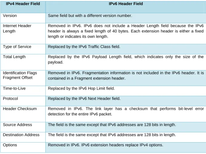
With all the enhancements that IPv6 brings, ideally IPv6 should be more effective and efficient to use. IPv6 has developed a lot of interest within the network research community including studies conducted by Murugesan, Ramadass and Budiarto (2009), Chengqing Yinglong and Jizhi (2007) and Narayan, Shang and Fan (2009). Jointly, these researchers focussed on evaluating and analysing the performance of a network that implements IPv6. The major concern is the size of IPv6‟s overhead, it doubles the IPv4‟s overhead size, and it may degrade a network‟s performance. However, these researchers have a totally different set of hardware and as a result; it is very hard to compare them. Table 2-4 shows the IPv4 Header fields and their corresponding IPv6 Header fields.
IPv4 Header Field IPv6 Header Field
Version Same field but with a different version number. Internet Header
Length
Removed in IPv6. IPv6 does not include a Header Length field because the IPv6 header is always a fixed length of 40 bytes. Each extension header is either a fixed length or indicates its own length.
Type of Service Replaced by the IPv6 Traffic Class field.
Total Length Replaced by the IPv6 Payload Length field, which indicates only the size of the payload.
Identification Flags Fragment Offset
Removed in IPv6. Fragmentation information is not included in the IPv6 header. It is contained in a Fragment extension header.
Time-to-Live Replaced by the IPv6 Hop Limit field. Protocol Replaced by the IPv6 Next Header field.
Header Checksum Removed in IPv6. The link layer has a checksum that performs bit-level error detection for the entire IPv6 packet.
Source Address The field is the same except that IPv6 addresses are 128 bits in length. Destination Address The field is the same except that IPv6 addresses are 128 bits in length. Options Removed in IPv6. IPv6 extension headers replace IPv4 options.
As shown in Table 2-3, four of the IPv4 Header fields are no longer in use in the IPv6 header, they are as follows: The Internet Header Length has been removed in IPv6 due to Table 2-3: IPv4 header field and its corresponding IPv6 header field. (Davies, 2008)
16 the fact that the header length in IPv6 is fixed to 40 bytes. The other three that have been removed are Identification Flags Fragment Offset, the Header Checksum field and the Option field. Table 2-4 below outlines some of the key differences between IPv4 and IPv6.
Internet Protocol version 4 Internet Protocol version 6
Source and destination addresses are 32 bits (4 bytes) in length.
Source and destination addresses are 128 bits (16 bytes) in length.
IPsec header support is optional. IPsec header support is required. No identification of packet flow for prioritized delivery
handling by routers is present within the IPv4 header.
Packet flow identification for prioritized delivery handling by routers is present within the IPv6 header using the Flow Label field.,
Fragmentation is performed by the sending host and at routers, slowing router performance.
Fragmentation is performed only by the sending host.
Has no link-layer packet-size requirements, and must be able to reassemble a 576-byte packet.
Link layer must support a 1280-byte packet and be able to reassemble a 1500-byte packet.
Header includes a checksum. Header does not include a checksum.
Header includes options. All optional data is moved to IPv6 extension headers.
ARP uses broadcast ARP Request frames to resolve an IPv4 address to a link-layer address.
ARP Request frames are replaced with multicast Neighbor Solicitation messages.
Internet Group Management Protocol (IGMP) is used to manage local subnet group membership.
IGMP is replaced with Multicast Listener Discovery (MLD) messages.
ICMP Router Discovery is used to determine the IPv4 address of the best default gateway and is optional.
ICMPv4 Router Discovery is replaced with ICMPv6 Router Solicitation and Router Advertisement messages, and it is required.
Broadcast addresses are used to send traffic to all nodes on a subnet.
There are no IPv6 broadcast addresses. Instead, a link-local scope all-nodes multicast address is used. Must be configured either manually or through DHCP for
IPv4.
Does not require manual configuration or DHCP for IPv6.
Uses host address (A) resource records in the Domain Name System (DNS) to map host names to IPv4 addresses.
Uses AAAA records in the DNS to map host names to IPv6 addresses.
Uses pointer (PTR) resource records in the IN-ADDR.ARPA DNS domain to map IPv4 addresses to host names.
Uses pointer (PTR) resource records in the IP6.ARPA DNS domain to map IPv6 addresses to host names.
Table 2-4 in the previous page shows some of the significant differences between IPv4 and IPv6. When looking closely at these differences, it can be seen that IPv6 was not designed Table 2-4: Comparing the main differences of IPv4 and IPv6. (Davies, 2008)
17 only to meet the demands for IP addresses. IPv6 was also designed for better performance, efficiency and security as well.
2.3 The Transmission Protocols
When travelling from home to work or home to school day by day, there are certain sets of rules to abide with as a road user. The vehicle that we use for transportation has its own set of rules to maintain. In this section of this chapter, this study will discuss and compare the two vehicles that will be used in this study for transmissions and they are, TCP and UDP. Within a computer network, protocol is a set of rules that oversee how data is delivered from sender to the receiver. The Open Systems Interconnection reference model was introduced by the International Standardisation Organisation (ISO) in the late 1970s. This reference model is widely used as a structure to relate all the functions that a computer network entails for data communication. Following is a brief explanation of the seven layers of the OSI model.
The application layer is responsible for the creation of the users‟ data, from word document to a simple e-mail to send via the network.
The presentation layer is the layer that is responsible for making communication between sender and receiver possible. For instance, encrypting and decrypting, protocol conversion and compression.
The session layer is responsible for opening and closing of the communication process between source and destination.
The transport layer is the one that is responsible for everything regarding the transportation of data from source to destination. For instance, the transport layer is required to divide the data into small pieces or packets before sending. When a packet arrives at destination host, the transport layer is responsible for putting these packets back together.
The network layer is where all the translation of addresses happens. The network layer is required to look at the address or name on the packet and translate it into a physical address (MAC address). In this layer also is where all the switching and routing is determined.
The data link layer is responsible for error correction as there may be errors created by the physical layer. These errors are corrected in the data link layer and determine other routes to send the packets through to its destination.
The physical layer is the lowest layer of the OSI model. This is the connection point of the other layers of the OSI model with the physical medium in the network such as, cables, and network interface cards.
Since the Internet came in to its existence, and due to its ever increasing rate, the Defence Advanced Research Project Agency (DARPA) decided to develop a simplified model and