APPLICATIONS OF DATA MINING TECHNIQUES IN TRANSPORTATION SAFETY STUDY
A Dissertation
Submitted to the Graduate Faculty of the
North Dakota State University of Agriculture and Applied Science
By Zijian Zheng
In Partial Fulfillment of the Requirements for the Degree of
DOCTOR OF PHILOSOPHY
Major Program: Transportation and Logistics
November 2018
North Dakota State University
Graduate School
Title
APPLICATIONS OF DATA MINING TECHNIQUES IN TRANSPORTATION SAFETY STUDY
By Zijian Zheng
The Supervisory Committee certifies that this disquisition complies with North Dakota State University’s regulations and meets the accepted standards for the degree of
DOCTOR OF PHILOSOPHY SUPERVISORY COMMITTEE: Pan Lu Chair Denver Tolliver Joseph Szmerekovsky Annie Tangpong Approved: 11/13/2018 Joseph Szmerekovsky
iii ABSTRACT
Most of current studies are based on Generalized Linear Models (GLMs), which require several assumptions. Those assumptions limit GLMs with the nature of data, and jeopardize models’ performance when handling data with complex and nonlinear patterns, high missing values, and large number of input variables with various data types. Data mining models are famous for strong capability of extracting valuable information and detecting complex patterns from large noisy data. However, they are not popular in transportation safety research, because they are criticized to be unable to provide interpretable and practical outputs. In this study, data mining models are tested in transportation safety research to prove their feasibility to be served as alternative models in safety study. Influential variable importance, contributor variable marginal effect analysis, and model predicting accuracy are further conducted to identify
complex and nonlinear patterns in study dataset, and to respond to the criticism that data mining models do not provide practical outputs.
Due to the high fatality rate, two types of crashes are selected as research areas: 1) predicting crashes at Highway Rail Grade Crossings (HRGCs); and 2) commercial truck involved crash injury severity.
In the HRGC crash likelihood study, three data mining models, Decision Tree (DT), Gradient Boosting (GB), and Neural Network (NN), are tested, and demonstrated to be solid in Highway Rail Grade Crossing (HRGC) crash likelihood study.
In the commercial truck involved crash injury severity study, the GB model identifies 11 out of 25 studied variables to be responsible for more than 80% of injury severity level
forecasting, and their nonlinear impact on the severity level. Several factors such as trucking company attributes (e.g., company size), safety inspection values, trucking company commerce
iv
status (e.g., interstate or intrastate), and registration condition are found to be significantly associated with crash injury severity. Even though most of the identified contributing factors are significant for all four levels of crash severity, their relative importance and marginal effect are all different. Findings in this study can be helpful for transportation agencies to reduce injury severity level, and develop efficient strategies to improve safety.
Keywords: safety, crash, prediction, big data, data mining, Decision Tree, Gradient Boosting, Neural Network.
v
ACKNOWLEDGEMENTS
First, I want to give my gratitude to Dr. Pan Lu, my advisor. Her utmost professionalism, considerable efforts, patient, wisdom and continuous encouragement have kept me moving forward during the study. What I learnt from her is going to be a fortune in my life, and I cannot express my gratitude enough. A very sincere thank you is due to my committee members for their guidance and support to improve the quality of this paper. Dr. Tolliver, Dr. Joseph, and Dr. Tangpong shared their experience and knowledge, and helped me to complete this thesis.
vi
TABLE OF CONTENTS
ABSTRACT ... iii
ACKNOWLEDGEMENTS ... v
LIST OF TABLES ... viii
LIST OF FIGURES ... ix
CHAPTER 1. INTRODUCTION ... 1
1.1. Transportation Safety ... 1
1.2. Data Driven Decision Making... 5
1.3. Transportation Safety Big Data ... 6
1.4. Current Research Limitations... 9
1.5. Data Mining... 11
1.6. Research Focus Area ... 14
CHAPTER 2. APPLYING DATA MINING TECHNIQUES IN HIGHWAY RAIL GRADE CROSSING ACCIDENT ANALYSIS ... 16
2.1. Introduction ... 16 2.2. Literature Review ... 20 2.3. Data Description ... 25 2.4. Methodology ... 27 2.4.1. Decision Tree ... 30 2.4.2. Gradient Boosting ... 33 2.4.3. Neural Network ... 35 2.4.4. Over-Fitting ... 36
2.4.5. Rare Event Predictions ... 39
2.4.6. Variable Importance Analysis ... 40
2.4.7. Model Prediction Accuracy ... 42
vii
2.5. Results Analysis ... 46
2.5.1. Decision Tree Results Analysis ... 46
2.5.2. Gradient Boosting Model Results Analysis... 52
2.5.3. Neural Network Model Results Analysis ... 60
2.5.4. Model Prediction Accuracy ... 69
2.5.5. Section Summary ... 73
CHAPTER 3. APPLYING GRADIENT BOOSTING IN COMMERCIAL TRUCK CRASH SEVERITY LEVEL ANALYSIS ... 75
3.1. Introduction ... 75
3.2. Literature Review ... 76
3.3. Data Description ... 82
3.4. Result Analysis ... 87
CHAPTER 4. CONCLUSIONS ... 104
4.1. Summary and Conclusions ... 104
4.2. Limitation and Future Study ... 107
viii
LIST OF TABLES
Table Page
1. Traffic Fatalities vs Age. ... 4
2. Input Variable Description ... 27
3. Classification Table ... 43
4. Variable Importance... 48
5. Effect of Factors on Crash Likelihood ... 50
6. Misclassification Rate vs Learn Rate and Complexity of Trees ... 54
7. Variable Importance Based on GB Model ... 56
8. Variable Importance (NN Model) ... 63
9. DT, GB, NN Model Prediction Classification Table ... 70
10. Model Prediction Accuracy Summary ... 71
11. Summary of Unanalyzed Variables ... 83
12. Variable Description ... 86
13. Variable Importance under Each Level of Severity ... 89
ix
LIST OF FIGURES
Figure Page
1. Injuries by Year, 1990-2016 ... 1
2. Fatalities by Year, 1975-2016 ... 2
3. HRGC Accident Count Nation Wide ... 17
4. HRGC Accident Count North Dakota ... 18
5. Structure of a Typical Decision Tree ... 30
6. Gradient Boosting Model Training Process (Alexander I) ... 34
7. Structure of Neural Network ... 36
8. Problem of Over-fitting... 37
9. Decision Tree Model Output ... 49
10. Partial Dependent Plots (GB Model) ... 59
1
CHAPTER 1. INTRODUCTION 1.1. Transportation Safety
Transportation safety is vital to transportation system operation performance. Traffic accidents cause traffic delay, property loss, and even people’s lives. In the U.S., there are more than 268 million registered vehicles, and 218 million people holding a valid driver license (Statista, 2017). The huge number of vehicles is one of the potential reasons leading to more traffic accidents. In 2015, there were approximately 6.3 million traffic accidents in the U.S. (Statista, 2017). On average, traffic accidents cost economy loss of 871 billion dollars each year (PBS, 2014), which is more than double of national public spending on transportation and water infrastructure at 416 billion dollars. (COB, 2015)
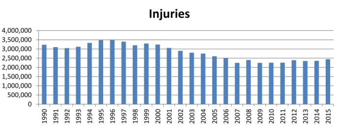
In addition to the high economy loss, traffic accidents also cause a huge number of injuries. As shown in Figure 1, traffic accidents caused more than 3 million injuries each year before 2002. Even though the number of injuries has decreased significantly since 2002, there are still more than 2 million of injuries each year. In addition, the trend shows the number of injuries started to rise after 2013.
Figure 1. Injuries by Year, 1990-2016
Source: Federal Highway Administration, 2016
0 500,000 1,000,000 1,500,000 2,000,000 2,500,000 3,000,000 3,500,000 4,000,000 19 90 19 91 19 92 19 93 19 94 19 95 19 96 19 97 19 98 19 99 20 00 20 01 20 02 20 03 20 04 20 05 20 06 20 07 20 08 20 09 20 10 20 11 20 12 20 13 20 14 20 15
Injuries
2
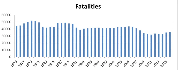
The most tragic fact about traffic accident is that it causes deaths. As automobiles became more popular in early twentieth century, traffic accident fatalities increased tremendously, and transportation safety did not attract enough public concern until late twentieth century, when more safety studies were conducted and more safety enhancements were implemented. Therefore, the number of people died in traffic accidents decreased significantly. However, nowadays, there are still a considerable number of deaths due to traffic accidents. As shown in Figure 2, traffic crashes took more than three million lives in the U.S. including more than 30,000 people killed on the roads of the United States each year (FHWA, 2016). In a typical month, traffic accident causes more death than the terrorist attack on New York and Washington on September 11th 2001. Every year traffic accident causes more than a million deaths around the world. It is estimated that as the total number of accidents increase due to the rapid growth of the number of motor vehicles in many formerly less-motorized countries, total death in traffic accident is likely to exceed 2 million by the year 2020 (WHO, 2001).
Figure 2. Fatalities by Year, 1975-2016
Source: Federal Highway Administration, 2016
0 10000 20000 30000 40000 50000 60000
Fatalities
3
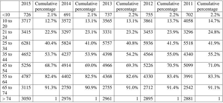
In addition, traffic accident is the fourth leading of cause of death, and is considered as one of the world's largest public health problems. Unlike the other top three cause of death (heart disease, cancer, and respiratory disease) the victims are overwhelmingly young and healthy prior to their crashes. According to Table 1, more than 50% deaths from traffic accidents are younger than 45 years old. Especially, approximately 13% of fatalities are younger than 20 years old.
4
Table 1. Traffic Fatalities vs Age. 2015 Cumulative percentage 2014 Cumulative percentage 2013 Cumulative percentage 2012 Cumulative percentage 2011 Cumulative percentage <10 726 2.1% 691 2.1% 737 2.2% 755 2.2% 702 2.2% 10 to 20 3717 12.7% 3572 13.1% 3565 13.1% 3861 13.7% 4058 14.7% 21 to 24 3415 22.5% 3297 23.1% 3331 23.2% 3453 23.9% 3296 24.8% 25 to 34 6281 40.4% 5824 41.0% 5757 40.8% 5936 41.5% 5518 41.9% 35 to 44 4652 53.7% 4237 53.9% 4398 54.2% 4564 55.0% 4340 55.2% 45 to 54 5256 68.7% 4914 69.0% 4966 69.3% 5226 70.5% 5099 71.0% 55 to 64 4787 82.4% 4402 82.5% 4368 82.6% 4330 83.4% 3991 83.3% 65 to 74 3115 91.3% 2750 90.9% 2755 91.0% 2712 91.4% 2542 91.1% > 74 3050 1 2976 1 2961 1 2895 1 2881 1
5
Since transportation safety drawn a lot of public attention, it has been improved with safety innovation implemented and drawn public awareness. However, during the past five years, the number of traffic accidents start back to increase. Thus, it is urgent to improve transportation safety in a further step. Traditionally, decision makings in transportation safety were relied on experience and limited number of available data. With developed computer technologies in early twenty-first century, data collection and storage techniques were innovated and improved, which enable data analysis and data-driven decision making more feasible and reliable than ever. 1.2. Data Driven Decision Making
Gilbreth et. al first started the study of scientific management, and contributed to the work that make decision making formalized and structured. Following their research, researchers were pursuing to model decision making mathematically and formulized. However, in 1970s, it was pointed out that not all the decision making problem can be quantitatively described in a mathematically formula. (Barnat, 2014). With the fast development and expansion of
information technology in late 90s, society production efficiency has been significantly improved due to automation management. Meanwhile, large amount of raw data recording the system activities was generated and recorded. However, these raw data was not summarized, analyzed, and evaluated in an appropriate way, which fails to convert the data to valuable information for decision makers. Therefore, data analysis and data driven decision making starts to drawn the concerns of researchers.
In transportation safety study, aiming to reduce the vast losses caused by traffic accidents, studies are taken from many disciplines. Solutions are sought from basic physical principles, engineering, medicine, psychology, human behavior, law, mathematics, logic, and philosophy, where data driven analysis can provide convincible and reliable results for decision makers. In
6
transportation safety, data driven analysis can be used with a wide range of purposes, and can be summarized into three main groups: descriptive analysis, explanatory analysis and predictive analysis. As most of raw data does not offer a lot of value before it gets processed, by conducting the three main analyses, valuable insights can be extracted from the raw data. Descriptive
analysis is usually the preliminary step to process the raw data to create and summarize, so that useful information can be provided and prepared for further analysis. Explanatory analysis can be used to better understand the data through a variety of algorithms. Explanatory analysis uses collected data, such as crash data, roadway data, and traffic data, to define crash related factors, and how these factors affect crash likelihood and outcomes. Unlike descriptive and explanatory analysis, predictive analysis focuses on what might happen in the future based on current research results.
In the past, crash and safety analysis were mostly relied on subjective or limited quantitative measures of safety performance, and limited number of data, which makes
researchers have difficulty in accurately evaluating each factor’ impact on safety when planning projects. Within the last decade, concept of big data gradually known by the public and its technology and application start to be mature and used in various fields. As data-driven analysis relies on real quality data, the big data provides foundation to data-driven analysis in
transportation safety study.
1.3. Transportation Safety Big Data
With the rapid development of information and computer technologies, people have been increasingly relying on information network. Meanwhile, the terminology of “big data” is
repeatedly mentioned and getting popular in various industries and in different situation. The term of “big data” is used to describe and represent the data with massive variety and volume
7
than traditional data, and can hardly be processed using old techniques and knowledge. An exact definition of "big data" is difficult to give because even within transportation safety field
professionals use it differently. Generally speaking, safety big data is a large dataset that can hardly be reasonably processed and managed using traditional techniques and knowledge, is a digital asset with a rapidly increasing value and requires new methodologies to store, obtain and process, so that it could assist with system optimization and decision making (Arthur, 2013). To be more specific, safety big data is a database integrated with multi-dimension datasets recording crash records, traffic history, environment, transportation infrastructure status, etc., and the actual safety big data will vary according to the use of purpose. The challenge when facing the massive scale and heterogeneous data is to surface insights and connections, which would not be possible using conventional methods (Ellingwood, 2016).
Safety big data is not only a simple big database as it seems like. Huge volume is only one of its characteristics. Doug Laney (2001) from Gartner company first presented "three Vs of big data" to describe three most important characteristics that make big data different from other data processing: volume, velocity, and variety. Every day, there are billions of trips generated in the U.S. Information of each trip is recorded in a certain format, such as text, video, audio, etc. Road sensors collect traffic information in time. GPS and smartphone apps record the path for each trip. When accidents happen, accidents information is collected by officers. Smart city is a new proposed concept expressing a new urban area in the future that uses different types of electronic data collection sensors to supply information which is used to manage assets and resources efficiently. Transportation will be an important component, and the interaction data between vehicles and transportation facilities and among vehicles each other will expands the safety big data in respective of volume, velocity and variety. Transportation safety is a
multi-8
discipline field. The safety data always includes data from other fields: engineering, human behavior, environment, geography, etc. Therefore, the safety big data expands not only within transportation industry, but evolves with many other fields.
In General, safety big data can be classified into two groups: structured and unstructured data (Taylor, 2017). Structured data are those that can be summarized, analyzed, stored, and accessed in a fixed format. Structured data’s format is always known in advance. For example, when analyzing effect of driver related factors on crash likelihood, the data can be structured as drivers with crash records and those without crash history. Computer languages and skills have been developed and achieved great success to process this kind of data. However, emerging issues are getting complicated and complex when such data extends to a huge size.
Unstructured data, on the other hand, are those without a pre-known form or structure. In an example of a group of data points representing drivers with and without traffic accident history, there are differences and features among these points to distinguish a certain group from the others. However, it is unknown that what the distinguished group is called, or what the rest of data is called. It could result from different genders or maybe age. Besides the huge size of unstructured data, deriving value from it through mathematical model is a huge challenge.
Safety big data provides foundation to enable decision making in transportation safety decided based on data and data analysis instead of experience and intuition. Nowadays,
researches on big data help transportation planners with state and local projects. With the help of safety big data, historical traffic data, census data and geographically data are integrated and analyzed, based on which driver behaviors are analyzed, road network is designed to achieve the balance between demand and supply, and planners can allocate limited resources more
9
Safety big data could find new solutions for improving transportation safety. With the safety big data concept, more achievements that are considered impossible or difficult can be made, such as real-time information interaction. More hidden trends and patterns are discovered and studied. With these findings, limited enforcement and management resources can be
allocated and controlled in a more efficient way. Another improvement that the safety big data brings to transportation safety is on warning, including warning to cars conditions, traffic
conditions, and drivers’ conditions. For example, digital maps could show the path and locations of vehicles carrying hazard materials, so that other drivers can make their own decisions to avoid potential dangers. Approximately 90% of car accidents are caused by human errors. In the future of unmanned vehicles, there will be more data generated each day between vehicles and vehicles, between vehicles and infrastructures, from each facility, and from each person. Human behavior will be substituted with computer system setups, which makes “human behavior” easy to be controlled. By setting up a driving speed limitation in the system of unmanned vehicles, over speed could be controlled better and possible to be monitored.
Even though safety big data is so critical, it can hardly provide any information that can be directly used by decision makers. Researchers have developed numerous mathematically models and algorithms to discover information from the data.
1.4. Current Research Limitations
“Big data is the key to a business success, big data will change the world, and big data will do this and that (Ghodke, 2015).” Nowadays, statements like this are popular. Although safety big data is important, it is the value extracted from the data that decision makers really need. To discover and explore information and patterns from the data, numerous models have been developed. Traditional Generalized Linear Models (GLMs) are considered as the most
10
popular models in transportation safety research. By building up a direct generalized linear relationship between target variable and independent variables, user can easily interpret and use this understandable quantitative relationship. However, GLMs heavily rely on the following assumptions (PSECS, 2017):
1) Independent variables are independently distributed.
2) The dependent variable does NOT need to be normally distributed, but it typically assumes a distribution from an exponential family (e.g. binomial, Poisson,
multinomial, normal, etc.)
3) GLM does not have to assume a linear relationship between the dependent variable and the independent variables, but it does assume linear relationship between the transformed response in terms of the link function and the explanatory variables. 4) Independent (explanatory) variables can be even the power terms or some other
nonlinear transformations of the original independent variables.
5) The homogeneity of variance does NOT need to be satisfied. In fact, it is not even possible in many cases given the model structure, and overdispersion (when the observed variance is larger than what the model assumes) maybe present. 6) Errors need to be independent but NOT normally distributed.
7) It uses maximum likelihood estimation (MLE) rather than ordinary least squares (OLS) to estimate the parameters, and thus relies on large-sample approximations. 8) Goodness-of-fit measures rely on sufficiently large samples, where a heuristic rule is
that not more than 20% of the expected cells counts are less than 5.
Once these assumptions are violated, it will generate numerous errors. In addition, when handling transportation safety big data, GLMs are limited by big data’s features, especially the
11
complicated non-linear patterns. Therefore, it is necessary to apply other models that can handle the big data, especially explore the non-linear patterns.
1.5. Data Mining
While GLMs show limitations when handling the safety big data, data mining models, a type of non-parametric data analytical models have been developed. Data mining is the process of discovering patterns and correlations, and extracting valuable information within large data sets (SAS, 2017). Data mining research was triggered as the large amount of data was generated and stored (emerging of big data), and the need of utilizing these data becomes urgent, because information extracted from the data can guild decision makers and bring large amount of profits to business.
The common data mining tasks can be divided into association analysis, clustering, classification, and prediction.
Association analysis is a meant to find frequent patterns, correlations, associations, or causal structures from various kinds of databases, such as relational databases, transactional databases, and other forms of data repositories (Techopedia, 2017). Given a set of data sets, association rule mining aims to find the rules which enable researchers to predict the occurrence of a specific item based on the occurrences of the other items in the data sets. For example, a red light violation are often found with drinking driving, because alcohol makes drivers make wrong decisions and slow down their reaction. Clustering or cluster analysis is the task to identify the attribute that can be used to separate a set of objects in a certain way, so that the objects in the same group are more similar to each other than to those in other groups in terms of certain attribute (Stefanowski, 2008). For example, clustering can be used when locate locations with high risk of crashes. Classification is the derivation of a function or model which determines the
12
class of an object based on its attributes (Fu, NA). A set of objects is given as the training set in which every object is represented by a vector of attributes along with its class. A classification function or model is constructed by analyzing the attributes and the class of objects in the data set. Such a classification function or model can be used to classify future objects and develop a better understanding of the classes of the objects in the database. For example, from a set of crash record data, which serve as the training data, a classification analysis can be built, which concludes each crash’s outcome (severity level). The generated classification model can be used to diagnose a new crash’s outcome based on the training crash record data, such as weather condition, traffic volume, type of vehicles, etc. Prediction is to discover the trend in a dataset, and build up a model to predict features of future data.
There are various data mining algorithms, such as K-means, support vector machine, neural network, classification tree, etc. (Li, 2015). Statistics and data mining share the same goal: discover and identify structure of the data and turn the data into valuable information. Even though data mining relies a lot on statistics theories, it utilizes knowledge from other fields as well, including machine learning, computer science, and database technology (Priyadharshini, 2017). In a statistics study, a hypothesis needs to be proposed and mathematic function and models are built up to test the hypothesis. In data mining, no hypothesis is pre-required. The links between target variable and its associated factors are automatically established.
Generalized Linear Models (GLMs) are the most popular statistical models favored by researchers in transportation safety study. GLMs are capable to construct quantitative
relationship between target variable and its contributor variables with mathematically equation. The inference reflects statistical hypothesis testing. The most favorable feature of GLMs is that the quantitative relationship is easy to interpret, so the outcome can be directly used by
13
researchers. It is easy to draw conclusions that can be used by decision makers. However, GLMs have several limitations. They can only handle structured data. When the data is complex, especially when it includes the mixture of interval, nominal, ordinal, and numerical variables, and there are a large number of redundant and irrelevant variables (Brusilovkey, NA), GLMs can low performance. GLMs’ performance can also be affected when the data is highly
heterogeneous and with high percentage of missing values, and outliers. As mentioned in previous sections, safety big data is usually noisy, and consists of a large number and various types of variables. In addition, the high percentage of missing values and a large number of redundant and irrelevant variables can all affect GLMs’ performance. In addition, GLMs are heavily relied on the pre-defined assumptions. When handling safety big data, all the pre-defined assumptions can hardly be satisfied at the same time. Once they are violated, it can cause
numerous errors.
Compared with GLMs, data mining models usually handle bigger size of data. In a GLM, a hypothesis has to be proposed before testing the model. Therefore, the noisy data type and redundant variables affect a lot on the model and variable selection. However, data mining models require no hypothesis. In fact, it can reveal the underlying pattern among variables. GLMs are mainly limited by the required pre-defined assumptions. On the contrary, data mining models are non-parametric, and they have no limitations on any pre-defined assumptions. Especially, data mining models are capable to discover non-linear complicated relationship between dependent variables and associated factors. In spite of the limitation of GLMs plus the strong capability of data mining models when handling big data, data mining models are not favored by researchers.
14 1.6. Research Focus Area
Even though data mining models are powerful when handling big data and have achieved success in many fields, application of data mining models in transportation safety research in still a gap. In a safety research, researchers still prefer to GLMs. The reason is that data mining outputs are hard to interpret. Data mining models can predict well but make a bad job when explaining the outcome (Shmueli, 2010). For example, one of the most popular data mining models, neural network, is always criticized because the blackbox in the model prevents people from understanding the model, even though the model can provide high prediction accuracy. Increasing model interpretability will trigger a better acceptance of the data mining models (Cortez & Embrechts, 2011). In this study, three popular data mining models, Decision Tree (DT), Gradient Boosting (GB), and Neural Network (NN) model, will be applied in
transportation safety research. Their robustness in mining safety big data will be tested. A few more analysis, such as variable importance and marginal effect, are conducted to provide better understanding of data mining models’ outputs.
Transportation safety is a big scope, and can be improved during processes, such as planning, design, facility construction, operation and infrastructure maintenance etc. This study will focus on two fields due to their severe influence on traffic and tragedy consequences: crash likelihood analysis at Highway-Rail Grade Crossings (HRGC) and injury severity level analysis of commercial truck involved crashes. The DT, GB, NN model Data mining models’ robustness will be first tested in the HRGC crash likelihood analysis. Then a model will be selected based on prediction accuracy, be tested in the commercial truck crash injury severity study using a bigger data.
15
1) Demonstrate the DT, GB, NN model feasibility in HRGC crash likelihood study. 2) Define the complicated and non-linear relationship between HRGC crash likelihood
and related factors.
3) Show that the DT, GB, and NN model can provide practical outputs by conducting further analysis in the study of HRGC crash likelihood, including contributor
variables’ marginal effect analysis, variable importance identification, and prediction accuracy.
4) Prove the GB model robustness in explaining commercial truck crash injury severity levels.
5) Identify explanatory variables of commercial truck crash injury severity levels, especially truck company characteristic and driver characteristic variables. Explore the relationship between truck involved crash severities and influential variables, especially the nonlinear relationship that cannot be identified by a GLM.
16
CHAPTER 2. APPLYING DATA MINING TECHNIQUES IN HIGHWAY RAIL GRADE CROSSING ACCIDENT ANALYSIS
2.1. Introduction
Highway-rail grade crossings (HRGCs) have long been recognized as critical transportation assets. The costs from disruptions to both the road and rail networks can be significant. In addition, the economic impact of those accidents is often compounded because of traffic delays on both the highway and railway. However, the high fatalities rate makes traffic accidents at these locations more catastrophic. From 1996 to 2014, there were 54,649 crashes at HRGCs across the United States where active warning devices (i.e. gates, lights, signs, bells, etc.) are in place (FRAOSA, 2015). About 12% of these crashes resulted in 6,527 fatalities (FRAOSA, 2015), while only 0.06% of all types of accidents lead to deaths. As shown in Figure 3, in the U.S., from 1996 to 2014, the number of HRGC accidents and resulted injuries and fatalities keep a decreasing trend with a little fluctuation in between. However, in North Dakota State, as shown in Figure 4, the number of accidents is not controlled well. Even though the number of accidents was low in 2006, it starts to increase since then. The fatality rate varies between 0% and 44%, and the fatality rate is higher than the national average for most of the time. Transportation agencies must identify the contributing factors to HRGC crashes to improve HRGC safety performance and reduce the number of crashes. A large volume of literature explores and evaluates the explanatory factors that contribute to the likelihood of HRGC collisions. Thus, an accurate HRGC accident prediction model is critical for HRGC safety improvement.
17 Figure 3. HRGC Accident Count Nation Wide
18 Figure 4. HRGC Accident Count North Dakota
Because crash accident data has random, discrete, and non-negative characteristics, Generalized Linear Models (GLMs) have been commonly selected to investigate the relationship between crashes and contributing factors. However, Lord and Mannering (2010) pointed out that, although the GLMs possess desirable elements for describing accidents, these models face
various data challenges which stem from crash data distribution and inappropriately fitted GLMs. Fitting the GLMs with data that exhibits a different distribution than the assumed distribution of the model can result in incorrect prediction and explanatory factors. As pointed out by Lu and Tolliver (2016) and Oh et al. (2006), HRGC crash data often shows under-dispersion distribution and less common GLMs are suitable for such datasets. Moreover, the available crash dataset is often containing a large portion of missing data and outliers. GLMs are sensitive to this noise. Outliers and missing values are often either deleted or imputed with the mean value. Furthermore,
19
to fit a well-performed GLM, a considerable number of observations are required. However, crashes at HRGCs are rare events. Event-level data, positive for a crash, are only a small portion of the entire dataset. The majority of data are at non-event level, representing zero crash. Thus, although some studies achieved remarkable overall prediction accuracy, the model only explains well for a non-event situation but was less accurate at the event-level (Chang and Chen, 2005; Chang and Wang, 2006; Chang and Chien, 2013). In addition, as one of important model
performance measurements, prediction accuracy is not analyzed thoroughly in previous studies. Data mining techniques have proven their robust ability to explore large, noisy, and complex data sets in recent years. Several data mining models have been applied in vehicle accident studies, including the neural network (NN) model (Chiou 2006; Zeng and Huang 2014), and the classification and regression decision tree (DT) models (Kashani, Rabieyan and
Besharati 2014; Yan, Richards and Su 2010). Appling data mining models to HRGC crash data modeling has received much less attention than GLMs. With the improvement of computing capability and software availability, data mining approaches are worth investigating with regard HRGC crash data modeling performance. Data mining approaches are used to find patterns in large datasets and relationships between target variables and predictors. Moreover, data mining approaches are a non-parametric method, which do not require any pre-defined underlying relationships between target variables and predictors, and the under-dispersed data does not affect model performance.
DT models are among the most favorable data mining models used in crash studies due to their capability to generate a visualized and easy-to-interoperate predictive-tree-based output and their effectiveness in handling non-linear interactions among variables with missing data. Using simple decision trees as fundamental components, the GB model improves the DT model in
20
terms of predicting capability while inheriting advantages of the DT model. NN models have a number of properties that make them very attractive over traditional GLMs. A NN is a non-linear processing system. Each layer in a NN represents a non-linear combination of non-linear
functions from the previous layer and requires no underlying theory about the data like most GLMs do. In addition, it is strongly capable of exploring patterns and requires little data clearness (SAS Institute Inc. 2015).
In this chapter, the DT, GB, and NN model are applied to predict crashes at HRGCs. Model performance in respect of forecasting accuracy is compared. In addition, influential variables are identified and their importance is compared. Moreover, further efforts to explore marginal effects with several traffic exposure factors and warning devices are also conducted in this chapter.
2.2. Literature Review
Studies of crash frequency at highway-rail crossings dates back to 1940s when the Peabody Dimmick Formula, one of the earliest predicting models for HRGC accident, was used to estimate the expected number of accidents based on historical crash data (USDOT, 1986). This model is developed based on accident data from rural rail-highway crossings in 29 states (USDOT, 1986). It uses three factors to forecast crash rate: Average Annual Daily Traffic (AADT), average daily train traffic, and the presence of warning devices. The developed relationship is as follows (Federal Highway Administration, 1986):
K P T V A 0.171 151 . 0 17 . 0 5 1.28 (Equation 1) Where A5 is the estimated number of accidents in 5 years. V is the Average Annual Daily Traffic (AADT). Tis the average daily train traffic. Pis the protection coefficient indicative of warning devices present. Kis the additional parameter.
21
Inspired by the Peabody Dimmick Formula, other models were developed based on similar theories and using similar factors, but with an adjustment of coefficient factors (Austin, 2002). Even though these models consider the major factors influencing crash rates, the resulting accuracy is still questionable, because of the limited number of explanatory variables. The U.S. Department of Transportation (USDOT) accidents prediction equations was a revolutionary model in this field and overcame previous shortcomings by taking more crossing design factors into account, such as type of warning devices, type of gate, and control type (USDOT, 1986). The USDOT accident prediction formula comprises of four equations (FRA, 1987; FRA, 1999):
) )( )( )( )( )( )( )( (K EI DT MS MT HP HL HT a (Equation 2) ) ( ) ( 0 0 0 0 T N T T T a T T T B (Equation 3) a T 05 . 0 0 . 1 0 (Equation 4) B
A0.7159 For passive devices;
B
A0.5292 For flashing lights;
B
A0.4921 For gates.
(Equation 5)
Where ais predicted number of accidents; Kis the Formula constant; EI is Exposure index factor; DTis Day through trains factor; MSis Maximum speed factor; MTis Main tracks factor;
HPis Highway paved factor; HLis Highway lanes factor;HTis Highway type factor. N , is the number of observed accidents in T years at the crossing, and T0 is the formula-weighting factor.
a, is determined on the basis of the various crossing-specific characteristics. B adjusts the predicted number of accidents (a) to reflect the actual accident history at the crossing. A
22
Although the USDOT accidents prediction equations were a great step forward in comprehensively explaining associated factors that impact crossing crash rate, they can hardly quantitatively measure the contribution that each factor makes to crash rate. This shortcoming is remedied by more recent regression models (Austin & Carson, 2002; Oh, Washington & Nam, 2006). Austin and Carson (2002) applied negative binomial accident prediction model in HRGC safety research. Compared to the USDOT accident prediction formula, their model made great improvement on interpretation of both of the magnitude and direction of the effect of significant contributor variables on HRGC accident frequencies. Their research defined traffic
characteristics, roadway characteristics, and crossing characteristics that are significant on affecting HRGC accident frequencies. Traffic characteristics, including night through train volume, AADT in both directions, number of tracks and traffic lanes, and train speed are found to be positively related with HRGC accident frequencies. Only one roadway characteristic variable was proved to be significant: if a highway is paved, the likelihood of accident is higher. For crossing characteristics, gates were proved to be effective on preventing accidents at HRGCs. However, presence of stop signs, flashing lights, or bells were all found to increase accident risk. Oh, Washington, and Nam (2006) tested gamma probability model in HRGC crash study by comparing it with previous models: Peabody Dimmick Formula, New Hampshire Index, NCHRP Hazard Index, USDOT prediction formula. Their research found out that AADT, presence of commercial area and train detector distance are significantly positively related with HRGC frequencies, while presence of track circuit controller, presence of guide, and presence of speed hump have a negative effect on the crash frequency. Although road and crossing width and number of tracks were found to be not significant, the authors believed that the effects of these factors were likely to be captured by the correlated variables, such as traffic and train volume.
23
Several other researchers also adopt GLMs (Raub 2009; Hu, Li and Lee 2012). In Lu and Tolliver’s study (2016), the different types of GLMs were compared and summarized, including Poisson model, negative binomial model, Conway-Maxwell-Poisson model, Bernoulli model, the hurdle Poisson model, and zero-inflated Poisson model. Poisson, Conway-Maxwell-Poisson, Bernoulli, and hurdle Poisson model were demonstrated to be able to handle under-dispersion issue. In a further comparison among these four models, the authors concluded that all models provided the same parameter sins for all the studied variables, such as AADT, train volume, number of tracks, and max train speed. The Bernoulli model and hurdle Poisson model showed almost identical results on parameter estimates. The Convey- Maxwell-Poisson model generated most distinctive parameter estimates for explanatory variables compared with the Poisson regression model. Crossing warning devices, highway traffic, rail traffic, train speed, number of tracks, appearance of paved highway, are all significantly related with HRGC accident likelihood defined by all four models. AADT, trains per day, number of tracks, paved highway, and
maximum train speed are all examined to be positive contributor variables.
Although GLMs are useful for predicting crash frequency and for interpreting relationships, the models often have low prediction accuracy and are often limited with
underlying data assumptions. The specification of the functional form depends on the nature of the data and can significantly affect the goodness-of-fit of GLMs and result in erroneous
parameter estimations and low prediction accuracy if the assumptions are violated (Xie, Lord and Zhang 2007).
With no pre-defined underlying data theory or assumptions, data mining algorithms start to gain popularity in accident frequency study. However, most of studies focus on highway safety and very limited on accident frequency at HRGCs (Chang & Chen, 2005; Li, Zhang & Xie,
24
2008; Chang, 2005). Within the limited number of studies on HRGC accident prediction based on data mining models, decision tree model is the most common selected method due to its ease-of-use tree structure result. Yan, Richards, and Su (2010) investigated crash frequency at HRGCs using two-stage classification and a regression decision tree model. Decision tree based results are generated and analyzed under three different scenarios. They find that the crash pattern and contributory factors are significantly different between cross-buck-only-controlled crossings and stop-sign-controlled crossings. However, DT method still contains few draw backs, even though the decision tree provides easy-to-view illustration, the tree structure is instable and sensitive to outliers. Moreover, DT method often produces a large and complex tree which still poses great presentation difficulties.
The GB model, an ensemble of simple decision trees, is extremely powerful in
understanding the structure of complex datasets and exploring potential relationships between dependent variables and independent variables, and is believed to be superior to simple DT models because of its techniques for handling missing data, robustness with data noise and resistance to over-fitting (Trevor, 2014).
Different with tree-based data mining models, NN model is inspired by mimicking human brain learning process. Codur and Tortum (2015), and Abdulhafedh (2016) apply neural network models to analyze highway accident frequencies. They identify influential factors of highway accidents, evaluate their models’ performance, and indicate that NN model do not impose the stringent distribution assumptions and can provide robust results with even chaotic input data such as a data with a lot of missing values. However, they fail to explore relationship between crash likelihood and influential factors because of the black box in the NN model. Fish and Glogett (2003) propose a method to look inside of the black box and analyze the effect of
25
input variables on target variable by keeping all other independent variables unchanged at certain level, and varying the studied independent variable within a range. Their method is used by Xie, Lord, and Zhang, and Chang’s study on highway accident frequency prediction (Xie, Lord & Zhang, 2007; Chang, 2005; Zhang & Meng, n.d.). However, Gevrey, Dimopoulos, and Lek (2003) point out that it is arguable and questionable when keeping the unstudied variables at a random or meaningless value. In addition, the explored relationship could be different when the unstudied variables are kept at various levels. Thus, they proposed a method to generate the relationship by keeping the other variables at meaningful values, such as mean value of the variable, and all the explored relationships are recorded while the remaining variables are held at different values.
In the following chapter, the DT, GB, and NN algorithms are described, and HRGC accident likelihood is predicted with all three algorithms. The model predictive accuracies are observed to be comparable among all three models and furthermore, result of each model and its performance are analyzed and compared thoroughly.
2.3. Data Description
This study uses 19 years of accident/incident data merged from the FRA’s Office of Safety accident/incident database and the FRA’s Office of Safety highway-rail crossing inventory. The data was merged by using the HRGC identification number in both of the databases. The merged database contains all the historical crash information at HRGCs in North Dakota from 1996 to 2014, including crossing location, traffic condition, infrastructure
equipment, accident information, time, and weather conditions. There were 5,713 HRGCs in North Dakota during that period, of which 354 have historical accident records. To study crash-associated factors and effectiveness of warning devices, a binary target variable (ACCIDENT) is
26
defined with two classes: a value of 1 indicates that there was a crash, while value of 0 represents a crossing with no crash. Table 2 lists all screened variables, including one target variable, one ID variable, and twenty-two input variables. These input variables can be divided into two categories: traffic characteristics, and crossing characteristics. Traffic characteristics record traffic information at crossings. These characteristics describe highway and railway traffic volume and traffic speed. Crossing characteristics describe presence of warning devices and other crossing related characteristics.
27 Table 2. Input Variable Description
Variable Property Description
ACCIDENT Target
variable
1= crash happened, 0=no crash
ID ID variable Crossing identification
Traffic Characteristics
AADT Numeric Annual average daily traffic
AVERAGE_TRAIN_SPEED Numeric Average train speed
DAYSWT Numeric Day switching train movements
DAYTHRU Numeric Day through-train movements
NGHTSWT Numeric Night switching-train movements
NGHTTHRU Numeric Night through-train movements
SCHLBUS Numeric Average number of school bus passing over
the crossing on a school day TOTAL_NUMBER_TRACK Numeric Number of rail tracks at crossings TRAFICLN Numeric Number of traffic lanes crossing railroad Crossing Characteristics
Highway_Paved Category Is highway paved or not? 1=yes, 0=no ADVWARN Category Presence of static advance warning Signs:
1=yes, 0=no
COMPOWER Category Commercial power availability: 1=yes, 0=no DOWNST Category Does track run down a street? 1=yes, 0=no FLASHMAS Category Presence of mast mounted flashing lights:
1=yes, 0=no
FLASHNOV Category Presence of cantilevered flashing light not over traffic lane: 1=yes, 0=no
FLASHOV Category Presence of canti-levered flashing light over traffic lane: 1=yes, 0=no
FLASHPAI Category Presence of flashing light in pairs: 1=yes, 0=no
GATES Category Presence of Gates: 1=yes, 0=no
Near_City Category In or near city? 1=near city, 0=in city
STOPSTD Numeric Highway stop signs presence: 1=yes, 0=no
WIGWAGS Numeric Presence of wigwags: 1=yes, 0=no
XBUCK Numeric Presence of cross buck: 1=yes, 0=no
2.4. Methodology
Every day, the safety big data is expending with new generated data. However, the pure data set can hardly provide any valuable information. In addition, traditional analytically GLMs
28
show limitations when handling big data. The concept of data mining starts to gain its popularity among various fields. With the goal to detect consistent patterns and relationships between variables, data mining is developed and defined as an analytic process to explore the huge, noisy, incomplete, and random data set. The first stage of data mining is initial exploration, which involves data cleaning, data transformation, data pre-screen, and problem definition. The second stage is model training and validation. In this stage, various data mining models are analyzed and an optimal model is selected based on model performance and assessment measurements. The third stage is deployment, where the optimal model in the second stage will be applied to a new data to generate predictions or estimations. The ultimate goal of data mining is prediction, which has the most direct business applications (Data Mining Techniques, 2018).
Statistics is quantitative analysis, interpretation, and summary of numbers or data. It provides fundamental definitions and concepts to data mining. However, even though both of data mining and statistics have the same goal: to discover and identify information from data, because of the 3 Vs characteristics of big data, traditional statistics models have limitations when handling big data. On the other hand, data mining uses scientific methods, processes, and
systems to extract knowledge from nasty data in various forms, either structured or unstructured. In addition, data mining is a multi-disciplinary field, which grew out of database technology. It covers a variety of tasks over statistics, such as data preparation, data inspection, and data cleaning.
Data mining methods can be generally divided into five categories: classification, estimation, association rules, clustering, and mining complicated data types. Classification is to classify raw data based on pre-defined categories. For example, insurance companies can use classification method to classify applicants to into customers with high and low risk of traffic
29
accidents. Estimation is similar to classification. The difference between the two concepts is that classification has pre-defined categories, and the number of categories is fixed. However,
estimation will output an unfixed number. For example, Walmart makes estimation on size of a household based on the family’s purchasing frequency and amount. In this case, the size of households is not a fixed number, and it could be one, two, etc. Association rule is to analyze a group of events that tend to happen together. For instance, when people shop at supermarkets, there could be certain patterns existing. Such as people who purchase eggs could possibly buy milk as well. Supermarket will use this analysis to arrange the display of goods, and promote sales. Clustering is to group a particular set of observations based on their characteristics, and aggregate them based on their similarities. The group could be pre-defined and unknown. Mining complicated data types includes text mining, graphic mining, audio mining, etc. By training the model with a big certain type of data set, the model will learn to recognize certain patterns existing in the data set, such as to train a model learn to recognize people’s hand writing.
Data mining has been successfully applied in various fields, such as industrial, business, education, military, etc. Nowadays, more innovative equipment and technologies make
transportation data collection more easily, making more transportation data generated every day. In the future, as unmanned vehicles and intellectual transportation system are getting mature, with vehicle to vehicle data, vehicle to infrastructure data, and vehicle to passenger data coming in, the size of big data will expend tons of times as today. Thus, data mining starts to draw more concerns in transportation field, especially when decisions and strategies in transportation are transferring from experience driven to data driven.
In this study, three popular data mining models are introduced and applied in transportation safety study.
30 2.4.1. Decision Tree
A decision tree is a hierarchical tree-based prediction model. There are two types of decision tree models: classification tree and regression tree. A classification tree is developed for categorical target variables, whereas a numerical target variable will be fitted with a regression tree. The target variable in this study is discrete with two outcome levels: crossings with a crash, and without a crash. Thus, a classification tree will be generated.
Generally, development of a decision tree involves three steps. The first step is tree growth. As shown in Figure 5, at the beginning, all data concentrates in the root node.
Figure 5. Structure of a Typical Decision Tree
Then, the dataset is broken down into child nodes by applying a series of splitting variables (splitters). Each child node will be treated as parent node for a further splitting. The principle behind splitting is to ensure each child node is as homogeneous as possible after
splitting. The ID3 algorithm measures entropy, expected entropy, and information gain to decide if a variable should be chosen as the splitter, and whether the node can be further split or not
31
(Sayad, 2010). Entropy measures the amount of unpredictability in an event. The higher the entropy value, the harder it is to predict the outcome of an event. If a sample is completely homogeneous, the entropy value is zero. For a variable Swith c distinct values, the entropy
) (S
E of Sis calculated as Equation (6): (Freitas, 2013)
c i i i p p S E 1 2 log ) ( (Equation 6)Where piis the probability of taking a certain value. iis the index number of options.
If variable S is divided into subsets: S1, … Scby certain splitter, the expected entropy (EH ) measures the expected unpredictability of thesecoutcomes of variableSafter splitting, and calculated as: (25)
) log ( 1 2
c i i i i p p a a EH (Equation 7)Where: ai is the number of observations in each subset S1, … Sc, and ais the total number of observations in parent node S.
The difference between EHand E(S)is called the reduction in entropy or information gain (I), shown in Equation (8). Information gain measures how much a splitter can help predict the outcomes. The variable that generates the highest information gain discriminates parent node into the most homogeneous child nodes. Thus, after computing the information gain for
candidate variables, the one with the highest information gain will be selected as the splitting variable.
EH S E
I ( ) (Equation 8)
A node with an information gain 0 is considered as a terminal node, which means no further splitting can be performed, and the data in each terminal node will be the most
32
homogenous. After applying steps above recursively, a saturated tree is obtained. The saturated tree provides a best fit to the training data, but also ends up over-fitting the data set. Thus, the data set is divided for training and testing. The training data is used for splitting the nodes, and testing data is for measuring misclassification rate in optimal tree selection step.
The recursive algorithm behind the decision tree model keeps splitting the data until it ends up with pure sets. The decision tree always classifies the training data perfectly, and reaches an accuracy of 100% for the training data. However, as the decision tree keeps splitting the data, the tree gets bigger and bigger, and it becomes more and more accurate for the training data. But at some point, predictions become less accurate on the data that hasn’t been used to train the tree. Thus, to avoid yielding a very large size tree, three parameters can be established. The first is the node size. If a node contains too few observations, splitting will not continue. The second is the number of nodes in the path between the root node and the given node. When this number equals the set-up value, splitting will be stopped. The third is to conduct significance test to test if all the observations in the node contain nearly the same target value or not. When the significance level value is equal to the set-up threshold, a further split will not be allowed.
After a sequence of pruned trees are established, the last step is to select the optimal one from the sequence of pruned trees, based on a measurement of the misclassification rate of testing data, so that the training data will not be over-fitted. As the tree grows larger and larger, the misclassification rate of training data decreases monotonically, indicating that the saturated tree always fits best to the training data. However, the misclassification rate for the testing data decreases first to a minimum value, and then keeps increasing and approaching a certain value. The depth of an optimal tree is decided when misclassification rates reach a minimal value for both training and validation data.
33 2.4.2. Gradient Boosting
The gradient boosting method is also known as multiple additive trees (MAT), and is a machine-learning data-mining technique for regression and classification problems proposed by Friedman (2002, 2003) at Stanford University. GB method theoretically extends and improves the simple DT model using stochastic gradient boosting (Friedman, 2002). GB produces a predictive model in the form of an ensemble of several weak-prediction, simple, tree-based models (Schapire 1999; Monteiro 2004). Therefore, the GB model inherits all of the advantages of tree-based models while improving in other aspects, such as forecasting accuracy (Friedman, Meulman 2003). Moreover, several other features make the GB model, including its: handling of large datasets without pre-processing, resistance to outliers, handling of missing values,
robustness to complex data, and resistance to over-fitting (Friedman, Meulman 2003; Salford-Systems)
A GB model can be viewed as a series expansion approximating the true functional relationship (Salford-Systems). In general, GB model starts by fitting the data with a simple decision tree model, which has certain level of error in terms of fitness with the data. The simple DT model is referred as a weak learner. A detail description of the algorithm of simple decision tree can be referred to section 2.4.2. Considering the errors having the same correlation with outcome value, the GB model then develops another decision tree model on the errors or the residuals of the previous tree. This sequential process will repeat itself until errors are minimized. This procedure is shown in Figure 6 (Alexander I, 2002).
34
Figure 6. Gradient Boosting Model Training Process (Alexander I)
The detailed algorithm of GB is described as follows (De’ath 2007; Hastie et al. 2009):
n n n n n x g x f x f( ) ( ) ( , ) (Equation 9)Where x is a set of predictors, and f(x) is the approximation of the response variable. g(x,n) are single decision trees with the parameter nindicating the split variables. n(n=1,2,…,n) are the coefficients, and determine how each single tree is to be combined. Loss function measures prediction performance, such as deviance. Friedman (2001) proposed a numerical optimization method called functional gradient descent, which is summarized below:
1. Initialize f0(x);
2. For n=1 to n (number of trees)
a) For i=1 to m (number of observations), calculate the residuals
) ( ) ( 1 ] ) ( )) ( , ( [ ~ x f x f i i i in m x f x f y L y ;
b) Fit a decision tree to ~ to estimate yin n.
35 d) Update fn(x) fn1(x)ng(x,n) 3. Calculate
n n x f x f( ) ( ) 2.4.3. Neural NetworkA typical NN structure is shown in Figure 7. Note the three parts: input layer,
intermediate (also called the hidden layer), and output layer. Each neuron in the input layer is one predictor, denoted as Xi in Figure 1. A hidden layer is a layer of neurons transferring information from inputs into outputs. Several hidden layers can be placed between the input and output layers. However, there is no specific guidance to determine the number of hidden layers and neurons. A typical approach is to choose the average number of input and output nodes. The value of a neuron in the input layer is transferred into hidden layers through a transformation function. The weight (Wij) represents the ratio of transformed value to the value of the input variable. The downstream is computed as the summation of the values of neurons in the upstream layer multiplied by with the corresponding connection weights (W in Figure 7). Information transfers from hidden layers to the output layer through an activation function. Activation functions could be an identity function, binary step function, logistics function,
ArcTan function et al. Different activation functions greatly impact the result and performance of entire model. In this study, the target variable is defined as a two-level variable: 0 and 1
indicating non-event level and event level, respectively. Thus, in this research, the binary step function is selected and expressed as Equation (10) (McCulloch & Pitts, 1943):
threshold x for threshold x for x f 1 0 ) ( (Equation 10)
Where x is predicted value. When x is greater than a defined threshold, the predicted output is 1, otherwise, 0.
36
The NN will be initialized with random weights and run through the model for the first time. This run is very unlikely to result in the optimal solution. Thus, in the following iterations, the model will change the weights to get a smaller error. This process will repeat numerous times until the desired output agrees within some predetermined tolerance. The entire procedure is called back propagation.
Figure 7. Structure of Neural Network 2.4.4. Over-Fitting
Over-fitting is a common problem in data mining. In predicting modeling, over-fitting happens when a model is too closely fit to limited set of data points or the true pattern of the data. However, this “perfect” model won’t perform well when fitting with other data sets. Over-fitting is more likely with nonparametric and nonlinear models that have more flexibility when learning a target function. As such, many nonparametric machine learning algorithms also include
37
To prevent over-fitting, there are two main concepts. The first concept is to train the data mining model with different data set. This concept includes: cross-validation, training with more data, and removing features. Cross-validation is a powerful preventative measure against over-fitting. The idea is to use the initial training data to generate multiple mini train-test splits. Use these splits to tune the model. In standard k-fold cross-validation, the data is partitioned into k subsets, called folds. Then, the model is iteratively trained the algorithm on k-1 folds while using the remaining fold as the test set (called the “holdout fold”). Training with more data won’t work every time, but training with more data can help algorithms detect the signal better. The idea is to add more relevant data to the training data set. However, if more noisy data added, it will result in more errors. Thus, it is necessary to keep the data clean. Unlike adding more data, removing features is the opposite by manually removing irrelevant features to improve models’
generalizability.
The second concept is to set up proper parameters to the models, so that the model will stop before it gets to over-fitting. This concept includes: early stopping and regularization.
38
In a data mining model, early stopping criteria represents when the model is set to stop training. The most common criteria is the number of training iterations. For a complex data mining model, such as the GB and the NN model, learning process is complicated and time consuming. When training with a large dataset, training time could be as long as a few hours or even days. However, .as shown in Figure 8, it may not take a lot of training iterations or time to reach a certain desired training error percentage. Therefore, in most studies, the early stopping criteria is set up, so that the training will stop after reaching the desired error percentage instead of reaching to the 0% training error model generated. In a DT model, the number of training iterations is also called tree depth by some researchers.
Regularization parameters are critical for avoiding over-fitting and for improving model performance. For the selected three data mining models, popular regularization parameters are: learning rate for the GB and NN model, and tree complexity for the GB model. Learning rate is also called shrinkage rate (SPM User Guide 2013). It controls how fast the model updated or improved after each stage. The value of learning rate ranges from 0 to 1. A small value of learning rate yields great improvement and minimizes loss function, but requires more iterations and computational time (De’ath 2007). Higher values, close to 1, result in over-fitting and poor performance (SPM User Guide 2013). Tree complexity represents the number of nodes per single simple tree. A tree with two nodes is the simplest tree, which has only one split variable (Hastie et al., 2009). As the GB model’s performance is controlled by both of learning rate and tree complexity, both learning rate and tree complexity rate must be balanced to avoid over-fitting. To detect interactions between variables, and to take full advantage of the GB model, a higher level of tree complexity and a low learning rate are suggested for experimentation (SPM User Guide, 2013). In this study, the model is tested under three values of learning rate: 0.05,
39
0.01, and 0.005, and five levels of tree complexity: 2, 4, 6, 8, and 15. The NN model is tested under three values of learning rate: 0.05, 0.01, 0.005, and 0.001, with the same purpose.
In this study, a combination of the two concepts is applied to avoid over-fitting in the study. This combined method starts with splitting the raw data into two: a training data and a testing data. Then, the models are tested under the training data and testing data, and under different regularization parameter setups at the same time. The optimal DT, GB, and NN are selected when both of training and testing errors are relatively low compared with all setup combinations. Both of the training and testing data are originated from the raw data, so it avoids involving irrelevant data to the model training. After training the model with training and testing data, a prediction error trend will generated like the one in Figure 8. The selection of training and testing data percentage is simulated by assigning the testing data percentage from 10% to 40% with 5% incremental. The optimal percentage is selected when both of predicting errors from training and testing data are relatively low. Early stopping parameter is set up; otherwise, the training process will keep running until the model fit the training data perfectly.
2.4.5. Rare Event Predictions
A data set, in which one class is exceptionally rare, is defined as unbalanced data
(Cieslak and Chawla, 2015). When fitting the data in traditional predictive model, decisions will be biased towards the majority class. This will result in a good prediction for the majority class, but a relatively poor prediction for the minority class, which can be observed in previous studies (Chang and Chen, 2005; Chang and Wang, 2006; Pande, Aty and Das, 2010; and Chang and Chien, 2013). Some of them even failed to forecast rare events. Specifying correct prior probabilities and decision consequences is generally sufficient to achieve correct prediction results of a rare class in a predictive model. Usually, prior probability is represented by the