Machine learning for transient discovery in Pan-STARRS1 difference imaging.

(1)

Deposited in DRO:

04 September 2015

Version of attached le:

Published Version

Peer-review status of attached le:

Peer-reviewed

Citation for published item:

Wright, D. E. and Smartt, S. J. and Smith, K. W. and Miller, P. and Kotak, R. and Rest, A. and Burgett, W. S. and Chambers, K. C. and Flewelling, H. and Hodapp, K. W. and Huber, M. and Jedicke, R. and Kaiser, N. and Metcalfe, N. and Price, P. A. and Tonry, J. L. and Wainscoat, R. J. and Waters, C. (2015) 'Machine learning for transient discovery in Pan-STARRS1 dierence imaging.', Monthly notices of the Royal Astronomical Society., 449 (1). pp. 451-466.

Further information on publisher's website:

http://dx.doi.org/10.1093/mnras/stv292

Publisher's copyright statement:

This article has been accepted for publication in Monthly Notices of the Royal Astronomical Society c: 2015 The Authors Published by Oxford University Press on behalf of the Royal Astronomical Society. All rights reserved. Additional information:

Use policy

The full-text may be used and/or reproduced, and given to third parties in any format or medium, without prior permission or charge, for personal research or study, educational, or not-for-prot purposes provided that:

• a full bibliographic reference is made to the original source

• alinkis made to the metadata record in DRO

• the full-text is not changed in any way

The full-text must not be sold in any format or medium without the formal permission of the copyright holders. Please consult thefull DRO policyfor further details.

Durham University Library, Stockton Road, Durham DH1 3LY, United Kingdom Tel : +44 (0)191 334 3042 | Fax : +44 (0)191 334 2971

(2)

Machine learning for transient discovery in Pan-STARRS1

difference imaging

D. E. Wright,

1‹

S. J. Smartt,

1

K. W. Smith,

1

P. Miller,

2

R. Kotak,

1

A. Rest,

3

W. S. Burgett,

4

K. C. Chambers,

5

H. Flewelling,

5

K. W. Hodapp,

5

M. Huber,

5

R. Jedicke,

5

N. Kaiser,

5

N. Metcalfe,

6

P. A. Price,

7

J. L. Tonry,

5

R. J. Wainscoat

5

and C. Waters

5

1_{Astrophysics Research Centre, School of Mathematics and Physics, Queen’s University Belfast, Belfast BT7 1NN, UK} 2_{The Institute of Electronics, Communications and Information Technology, Queen’s University Belfast, Belfast BT3 9DT, UK} 3_{Space Telescope Science Institute, 3700 San Martin Drive, Baltimore, MD 21218, USA}

4_{GMTO Corporation, 251 South Lake Avenue, Suite 300, Pasadena, CA 91101, USA}

5_{Institute for Astronomy, University of Hawaii, 2680 Woodlawn Drive, Honolulu, HI 96822, USA} 6_{Department of Physics, Durham University, South Road, Durham DH1 3LE, UK}

7_{Department of Astrophysical Sciences, Princeton University, Princeton, NJ 08544, USA}

Accepted 2015 February 9. Received 2015 February 9; in original form 2015 January 15

A B S T R A C T

Efficient identification and follow-up of astronomical transients is hindered by the need for humans to manually select promising candidates from data streams that contain many false positives. These artefacts arise in the difference images that are produced by most major ground-based time-domain surveys with large format CCD cameras. This dependence on humans to reject bogus detections is unsustainable for next generation all-sky surveys and significant effort is now being invested to solve the problem computationally. In this paper, we explore a simple machine learning approach to real–bogus classification by constructing a training set from the image data of∼32 000 real astrophysical transients and bogus detections from the Pan-STARRS1 Medium Deep Survey. We derive our feature representation from the pixel intensity values of a 20 × 20 pixel stamp around the centre of the candidates. This differs from previous work in that it works directly on the pixels rather than catalogued domain knowledge for feature design or selection. Three machine learning algorithms are trained (artificial neural networks, support vector machines and random forests) and their performances are tested on a held-out subset of 25 per cent of the training data. We find the best results from the random forest classifier and demonstrate that by accepting a false positive rate of 1 per cent, the classifier initially suggests a missed detection rate of around 10 per cent. However, we also find that a combination of bright star variability, nuclear transients and uncertainty in human labelling means that our best estimate of the missed detection rate is approximately 6 per cent.

Key words: methods: data analysis – methods: statistical – techniques: image processing – surveys – supernovae: general.

1 I N T R O D U C T I O N

Current transient surveys such as Pan-STARRS1 (PS1; Kaiser et al.

2010), PTF (Rau et al.2009), LSQ (Baltay et al.2013), SkyMapper (Keller et al.2007) and CRTS (Drake et al.2009) are efficient dis-coverers of astrophysical transients. To make these surveys possible

_E-mail:_{[email protected]}

it has become necessary to automate every step in the data pipeline including data collection, archiving and reduction. A major goal for time-domain astrophysics is early detection and rapid follow-up to enable complete data sets for transients. Artefact rejection has become the bottleneck between fast transient detection and our ability to feed these targets to follow-up surveys such as PESSTO (Smartt et al.2013) and PTF for early classification. Current arte-fact rejection typically involves deriving some set of parameters from the image data of individual detections and thresholding each

2015 The Authors

at University of Durham on September 4, 2015

http://mnras.oxfordjournals.org/

(3)

parameter, only promoting those detections that pass the thresholds to humans for verification.

The numbers of detections that must be scanned by humans is still on the order of hundreds of objects each night with a high false positive rate. The processing artefacts produced are a result of many factors such as saturated sources, convolution issues and detector defects amongst others, and to a large extent are common across all surveys. For the next generation of survey, we cannot expect humans to remain involved in this process of artefact rejection to the same extent, where for example we expect of the order of 106

transient detections per night from LSST.1

Significant effort has been devoted to this problem in anticipa-tion of these next generaanticipa-tion surveys, and to enable rapid turnaround from detection to classification for current surveys. Machine learn-ing techniques have been used to take advantage of the large amounts of data gathered by these surveys to train a classifier that can distinguish real astrophysical transients from artefacts or ‘bo-gus’ detections. Examples include Donalek et al. (2008) for the Palomar-Quest survey, Romano, Aragon & Ding (2006) for SNFac-tory, and Bailey et al. (2007) and du Buisson et al. (2014) for SDSS. PTF have demonstrated the ability to efficiently characterize de-tections and initiate rapid follow-up, see Gal-Yam et al. (2014) for example, where the problem of real–bogus classification has been addressed by the work of Bloom et al. (2012) and Brink et al. (2013). While these studies do achieve high levels of performance, the pa-rameters chosen to represent the images are often dependent on the specific implementation and strategy of the individual surveys.

In this paper, we investigate a simple representation of the im-ages by using the pixel intensities in a region around a detection in a single difference image. This choice of parametrization is inde-pendent of other aspects of the survey, and is therefore applicable to any survey performing difference imaging while also lending it-self to implementation much earlier in the data processing pipeline (potentially at the source extraction stage). We begin by outlining the real–bogus problem in the context of PS1 in Section 2, followed by a description of our training set and image parametrization in Section 3. In Section 4, we discuss the various machine learning algorithms we investigate, outline how we select the optimum clas-sifier and report its performance compared with previous work. We continue in Section 5 with some further analysis to help under-stand how we expect the classifier to perform on a live data stream. Finally, we summarize our results and conclude in Section 6.

2 P S 1 A N D T H E P R O B L E M O F R E A L – B O G U S C L A S S I F I C AT I O N

The PS1 system comprises a 1.8 m primary mirror (Hodapp et al.

2004) and a field of view of 3.3 deg imaged by 60 4800×4800 pixel detectors, constructed from 10µm pixels subtending 0.258 arcsec (for more details, see Magnier et al.2013). The PS1 filter system consists of five filters,gP1,rP1,iP1,zP1similar to SDSSgriz(York

et al.2000) with the addition ofyP1, which extends redwards of zP1. The system is described in detail by Tonry et al. (2012b).

The PS1 Science Consortium (PS1SC) operates the PS1 telescope performing two major surveys. The Medium Deep Survey (MDS; Tonry et al.2012a) is allocated 25 per cent of observing time for high-cadence observations of 10 fields, each the size of the PS1 field-of-view. The wide-field 3πsurvey with 56 per cent observing time aims to observe the entire sky north of−30 deg declination

1_{http://www.lsst.org/lsst/}

with a total of 20 exposures per year in all five filters for each pointing.

In this paper, we use images from the MDS. Each night three to five of the MDS fields are observed. Each epoch is composed of eight dithered exposures of 8×113 s ingP1andrP1, or 8×240 s

iniP1,zP1andyP1, producing nightly stacked images of 904 and

1632 s duration (Tonry et al.2012a). Each stack achieves 5σdepths of around 23.3 mag ingP1,rP1,iP1,zP1and 21.7 mag inyP1. Images

from the PS1 system are processed by the Image Processing Pipeline (IPP; Magnier2006), on a computer cluster at the Maui High Perfor-mance Computer Center (MHPCC). The images are passed through a series of processing stages including device detrending, masking and artefact location. Detrending includes bias correction and flat-fielding using white light flat-field images from a dome screen, in combination with an illumination correction obtained by rastering sources across the field of view. After deriving an initial astrometric solution, the flat-fielded images are then warped on to the tangent plane of the sky using a flux-conserving algorithm. The plate scale for the warped images was originally set at 0.200 arcsec pixel−1_,

but has since been changed to 0.25 arcsec pixel−1_{in what is known}

internally as the V3 tessellation for the MDS fields. Bad pixels are masked on the individual images and carried through the stacking stage to give the nightly stacks.

Difference imaging is performed on a daily basis by two indepen-dent pipelines. IPP takes the nightly stacks and creates difference images by subtracting a high-quality reference image from the new data. Point spread function (PSF) photometry is then performed on the difference images to produce catalogues of variables and transient candidates (Gezari et al.2012; McCrum et al.2014). The Transient Science Server (TSS) developed by the PS1SC ingests catalogues of detections of residual flux in the difference images and presents potential transients for human eyeballing.

In parallel, an independent set of difference images are produced at the Centre for Astrophysics at Harvard from the nightly stack images using thePHOTPIPE (Rest et al. 2014, 2005) software. A

custom-built reference stack is produced and subtracted from the IPP nightly stack to produce an independent difference image. This process is described in Gezari et al. (2010,2012), Chomiuk et al. (2011), Berger et al. (2012), Chornock et al. (2013) and Lunnan et al. (2013), and potential transients are visually inspected for promotion to the status of transient alert. A cross-match between the TSS and thePHOTPIPEtransient streams is performed and agreement

between the detection and photometry is now excellent, particularly after the application of uniform photometric calibration based on the ‘ubercal’ process (Schlafly et al.2012; Magnier et al.2013).

2.1 Artefacts in difference imaging

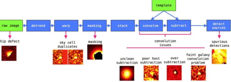
In this work, we only use detections from IPP difference imaging and not the independentPHOTPIPEdetections. In Fig.1, we show a

modular diagram of IPP difference imaging process and the sources of the main types of artefact.

The first source of bogus detections are chip defects, which take various forms. After detrending, the chip data are resampled and geometrically warped to fit a unit area of sky that the data are projected on to, known as a sky cell. Occasionally, a transient will lie on a region of the detector that when projected on to the sky falls on overlapping sky cells. This results in duplicate warp images of the same chip data, with the object lying close to one of the sky cell edges. After warping, sky cell edges, chip defects and saturated sources are masked. Masked pixels in individual exposures are propagated through the stacking stage.

(4)

Figure 1. Modular diagram of the IPP difference imaging steps and the types of artefacts arising from each stage.

A kernel is derived to degrade a high-quality template image to match the nightly stack. The template is convolved with this kernel and subtracted from the nightly stack. This series of steps leads to a class of artefacts which we refer to as convolution issues. In general, these arise from the derived kernel not being able to accurately match all sources in the template to those in the nightly stack. This causes problems with bright sources where the kernel is unable to fit the entire PSF of the detection in the nightly stack image. These artefacts appear as high signal-to-noise (S/N) PSFs but with darker rings appearing in the wings, an example is shown in the bottom panel of Fig.4. We call these unclean subtractions. The flux in these detections is probably due to a bright stellar variable. Identifying variable stars (and AGNs) is quite a different problem to detecting transients and we have chosen not to try to tailor our algorithms to do both. The efforts in this paper are focused on finding transients, although inevitably stellar variables from very faint host stars are detected. Hence we discard these bright stellar variables that appear in the difference images as they are straightforward to identify. We find these detections make up∼10 per cent of the bogus detections. The same convolution issues can lead to poor host galaxy sub-traction, where an inadequately convolved host can be over or un-dersubtracted leaving a pattern of positive and negative flux. This makes it difficult to disentangle any potential real detection. The third convolution issue we highlight in Fig.1arises when point-like sources in the template image are broader than that of the nightly stack resulting in an oversubtraction in the wings of the source in the difference image. This happens when observing conditions have been particularly good and the nightly stack is of higher quality than the template image (this is not a frequent occurrence). The final artefacts from the convolution and subtraction stage are convolution problems in the cores of faint galaxies, manifesting themselves as faint nuclear transients and appearing as positive flux in the differ-ence image. Here the convolution step matches the morphology of the faint galaxy in the template and nightly stacks well; however, the peak flux of the convolved template is lower than that in the nightly stack. This results in the nucleus of the faint galaxy being undersub-tracted leaving residual flux in the difference image. These artefacts are the most difficult to identify by eye but are distinguished by a narrower PSF than expected. It is not always clear if the flux is due to real variability or an artefact of convolution, in any case these targets could not be confidently selected as real transients for follow-up. This highlights one of the major uncertainties in training

the algorithms – secure labelling of real and bogus objects, which we return to in Sections 5.3 and 5.5.

Another source of artefacts arises during the source extraction phase. Flux in the nightly stack from diffraction spikes for example that have no equivalent in the template image get flagged as potential transients. We refer to these as spurious detections in Fig.1.

Our approach to date for removing these contaminants has been to attempt to derive a set of filters based on image statistics de-rived for each potential transient detection by IPP. These filters normally take the form of threshold values for some parameters (see Section 2.2). However, the parameter space is typically large and the work required to manually develop the optimal set of fil-ters is impractical. Despite this our current hand-engineered checks allow only a small fraction of the bogus images through. This still produces of the order of a few hundred bogus objects each night passing the cuts and being presented to human scanners for veri-fication. This is approaching the limit of what can comfortably be processed by humans on a daily basis and clearly a solution needs to be found for the next generation of survey.

Over the course of the last∼3 years of the PS1 survey we have accumulated a large amount of data associated with a few tens of thousands of astronomical sources that have either been classified as real objects or artefacts using a combination of the cuts detailed in Section 2.2 and human scanning. This readily available data lends itself to data-mining where we hope to use the historic data to improve on the current method of real–bogus classification. In Section 2.3, we outline how supervised learning can be applied to this archive of PS1 data in order to construct a real–bogus classifier that can be applied to the nightly stream of new data gathered from PS1 and future surveys. First, we describe the cuts we perform.

2.2 Cuts

Prior to ingesting detections from IPP difference imaging into a

MYSQLdata base at Queen’s University Belfast (QUB), we perform

pre-ingest cuts based on the detection of saturated, masked or sus-pected defective pixels within the PSF area. Taking as a typical night 2013 September 3 [56548 MJD (Modified Julian Date)], the seven nightly stacks produced 366 267 detections (∼52 000 detec-tions per stack), the pre-ingest cuts rejected 94.88 per cent of these detections.

(5)

The∼18 750 detections passing the pre-ingest cuts are associated with transient candidates if there are two or more quality detections within the last seven observations of the field, including detections in more than one filter, and an rms scatter in the positions of≤0.5 arcsec. Each quality detection must be of more than 3σsignificance and have a Gaussian morphology (XYmoments<1.2). These post-ingest cuts also include checks for convolution issues, proximity to bright objects and ‘NaN’ values close to the centre of bright PSFs. 63 per cent of the detections that passed the pre-ingest cuts were rejected during the post-ingest cuts. The remaining detections were promoted for human screening, where 37 per cent of the detections were deemed to be real. These real transient candidates are cross-matched with catalogues of astronomical sources in the MDS fields. We use our own MDS catalogue and also extensive external cata-logues (e.g. SDSS, GSC, 2MASS, NED, Milliquas,2_{Veron AGN,}

X-ray catalogues) to make a contextual classification of supernova (SN), variable star, active galactic nuclei (AGNs) or nuclear tran-sient. We also cross-match with the Minor Planet Centre to reject asteroids, though most are removed during the construction of the nightly stacks.

2.3 Supervised learning for classification

In general, supervised learning entails learning a model from a training set of data for which we provide the desired output for each training example. For the purposes of designating a detection as a real transient or a processing artefact, the desired output for each image is discrete. In such cases, the problem is a supervised clas-sification task for which there are a vast array of machine learning algorithms. In Section 4, we discuss the algorithms we try; however, all such algorithms are trying to learn a model from the training data that will allow them to map the input parametrization of each train-ing example (see Section 3.2) to the desired output orlabel, while at the same time ensuring the model performs well on data not seen during the training phase. For building a real–bogus classifier, this is an obvious avenue to pursue as we have a large sample of historical data for which we have labels provided by our current cuts and also through human eyeballing.

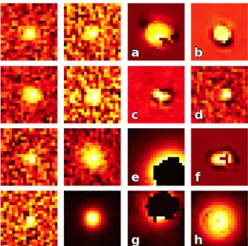
In Fig.2, we show a sample of both real and bogus examples drawn at random from the training data. Often bogus detections show a combination of the factors we describe in Section 2.1 and typically this affects the centroiding during the source detection stage.

3 T R A I N I N G S E T A N D F E AT U R E R E P R E S E N TAT I O N

As discussed in the previous section, we must provide a labelled training set from which the classifier can learn to recognize the characteristics that can identify detections as being members of one of the classes: real or bogus. In order to learn a model that will generalize well to detections in new observations, it is important that detections in the training set are representative of all detections we expect to see. In practice, this is easiest to achieve by providing the learning algorithm with the largest possible training set, indeed Brink et al. (2013) attribute much of their improvement in perfor-mance over Bloom et al. (2012) to using a training set with two orders of magnitude more training examples. In the remainder of this section, we describe the compilation of the training set, starting

2_{http://quasars.org/milliquas.htm}

Figure 2. Example detections randomly selected from the training data. The two columns on the left show examples labelled as real and the two on the right show those labelled as bogus. Bogus detections a–c and f show signs of oversubtraction, with a and f also showing masking. d is a faint galaxy convolution problem. Detections e and g are saturated sources that have been masked. Finally, h is an example of an unclean subtraction of a bright star.

with a description of our training example selection process and labelling.

3.1 Training set

Over the past 3 years ∼1 million potential transients have been catalogued in the MDS by the TSS. Approximately 8000 of these objects have been selected by humans as real transients and pro-moted as potential targets for spectroscopic follow-up. As of the end of the survey in 2014 May, 515 transients had spectroscopic classifications.

The aggregate catalogue information for all objects extracted by IPP and which pass the pre-ingest cuts described in Section 2.2 are stored in a data base at QUB. Individual detections are associated with an object if they are spatially coincident within 0.5 arcsec. This information is presented to humans in the form of webpages.3

The webpages show all the photometric points produced by IPP in a multicolour light curve. The number of photometric detec-tions typically ranges from a few to a few dozen depending on the magnitude and time-scale of the transient objects (see Chomiuk et al.2011; McCrum et al.2014; Rest et al.2014; for examples of light curves). These webpages also present a subset of the image postage-stamps of the detections associated with an object (target image, reference image and difference image). This subset contains the first detections of the object of which there are always at least two (see Section 2.2) and up to five subsequent detections. Each object is then eyeballed by a human, those that appear to be real

3_{Similar webpages are made public for the PS1 3Pi Survey at} http://star.pst.qub.ac.uk/ps1threepi/psdb/public/

(6)

transients are promoted as potential targets for scientific follow-up, while artefacts are discarded.

Our training examples are drawn from the subset of detections we choose to present on the human digestible webpages for each object, as detailed above (typically two to three but less than seven). The majority of real examples were taken from detections of promoted objects with no spectroscopic classification. There is no guarantee that all detections of a promoted object are necessarily a result of good image subtractions. This prohibits simply assigning a label of real to all individual detections associated with a promoted target. In order to ensure that we have a secure, reliable and clean set of real detections for training, we inspected and individually labelled 4352 detections (from 1919 different transients) as real, discarding any artefacts from the training set. We augmented this sample of real detections with data from 53 spectroscopically confirmed SNe (from 2012 December to 2014 January) for which we used the complete set of detections (∼31 detections per object on average). These were again manually checked to remove bogus detections. We held out the first detections of all 53 SNe, which we use for testing in Section 5.7 and all detections of PS1-13avb, which we use in Section 5.6. This leaves an additional 1603 real training examples bringing the total to 5955 real detections.

Over the course of the survey approximately 800 000 objects have been discarded as artefacts providing of the order of 106_examples

of bogus detections. We randomly sample from the available bogus examples and aim for four times more bogus examples as real, this is similar to the proportions used by Brink et al. (2013). Initial tests with classifiers showed that a significant proportion of the false positives appeared to be clean subtractions. We improved the purity of the bogus sample by examining the randomly selected bogus detections and added any detections that looked like real transient subtractions to the list of real examples (the effect of label contamination is further discussed in Section 5.3). This produced an extra 464 examples for the set of real detections resulting in a final total of 6419. We then selected four times as many bogus images from the remainder of the bogus examples we inspected, producing a sample of 25 676 bogus detections.

The final training set contains 32 095 training examples. We divide the training examples into two sets, distributed as follows: 75 per cent for training and cross-validation, and 25 per cent for test-ing. The training examples are randomly shuffled prior to splitting with the caveat that all detections on the same night of a given object are included in the same set. This is to avoid detections with almost identical statistics being in multiple sets and giving a false impres-sion of a classifiers performance. The construction of the data set is summarized in Table1. The label for each training example is a 1 or 0, with 1 representing a label of real and 0 bogus.

The training set we have constructed is representative, containing examples of detections from different chips, seeing conditions and filters, with various levels of S/N and examples of all types of processing artefact.

Table 1. Composition of data sets.

Set Real Bogus Total

Training 4800 19 271 24 071

Test 1619 6405 8024

Total 6419 25 676 32 095

3.2 Feature representation

Machine learning algorithms require a one-dimensional (1D) vector representation of each training example, where each element of the vector corresponds to some numeric data orfeaturethat may be useful to the algorithm for discerning examples belonging to each class. Previous work in the area of real–bogus classification has focused on using parameters contained in catalogues generated by the processing pipeline and more complex features derived from that information to represent the detections, see table 1 from Brink et al. (2013) and table 1 from Romano et al. (2006).

The catalogue features available to individual surveys depend on the implementation of their IPP. When applying machine learning for real–bogus classification to a new survey it may not be possible to calculate these features based on the information available in the catalogues. There is also potential to spend a lot of time deriving and testing ways to combine the catalogue information that is available into features that we hope capture the differences between real and bogus detections. Bogus detections are the result of many factors and establishing a set of features that can encapsulate them all is dif-ficult. In contrast simply representing the detections by their pixel intensity values requires no time spent developing or tuning feature extractors. Previous work that relies solely on the pixel data has proven effective for simple visual classification tasks, such as hand written digits (LeCun et al.1998). For more complex tasks or to boost performance much of this work has been performed by learn-ing a hierarchy of unsupervised features from the pixel data (LeCun et al.1998; Coates, Lee & Ng2011). Establishing a firm benchmark on the pixel intensity representation allows us to assess the poten-tial gains from applying these more complex methods and is the main focus of this paper. Using this representation, we expect the learning algorithm to identify salient relationships between pixels for the classification task. In the next section, we discuss our choice of features and continue in the following section by describing the preprocessing steps we apply before training.

3.2.1 Feature vector construction

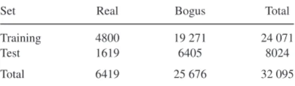
To represent our training examples, we use the pixel data itself. For a given training example, we construct its feature vector by selecting a 20×20 pixel area (corresponding to∼5 times the average seeing of PS1) around the centre of what IPP considers a transient, which we refer to as a substamp. The 1D vector is constructed by shifting off each column of the substamp and concatenating those columns together to produce a 400-element vector of pixel intensity values.

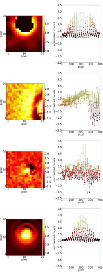
In Fig.3, we show visualizations of these feature vectors along with the substamp from which they were constructed for examples of real detections and for various levels of S/N. In Fig.4, we show detections labelled as bogus with examples of different types of artefact. A learning algorithm will learn to identify patterns in the feature vectors that are characteristic of examples belonging to the two classes.

The choice of feature representation is independent of the imple-mentation of the rest of the IPP and survey, with the assumption that the pixel level data is easily accessible.

3.2.2 Feature preprocessing

Aside from the image processing steps carried out by the pipeline, we carry out two additional transformations of the data. We first replace any ‘NaN’ pixel values with 0s. ‘NaN’ pixel values typi-cally arise from masking or floating point overflows during image

(7)

Figure 3. Visualization of feature vectors for detections labelled as real. The feature vectors are constructed by shifting off each column of the 20×20 pixel substamp on the left and appending them together to produce the 400-element 1D feature vector depicted on the right.

Figure 4. Similar to Fig.3but for bogus examples.

(8)

processing. We choose to replace these pixel values with 0 so as not to influence the next step in the preprocessing phase. As a sec-ond step, we apply a feature normalization function which allows classifiers to focus on relative pixel intensities and limits the effect of absolute brightness on the classifiers. We apply the following normalization: f(x)= x |x|log 1+|x| σ , (1)

wherexis a feature vector andσ is the standard deviation of the pixel intensity values for that feature vector. This is the same nor-malization function used byEYE4(Bertin2001) and similar to that

of Romano et al. (2006).

4 O P T I M I Z AT I O N O F T H E C L A S S I F I C AT I O N S Y S T E M

In order to achieve the best performance from the machine learn-ing algorithms discussed in the followlearn-ing sections, it is necessary to optimize the hyperparameters of each. This is done by a pro-cess known as cross-validation which is a brute force search of the hyperparameter space, where a model is trained with the hyperpa-rameters selected at predetermined intervals within the space. The best combination is selected by measuring the performance in a held-out sample of the 24 071 training examples.

Below we give a brief introduction to each of the classifiers. We also point out the free parameters that must be selected by cross-validation and discuss this process in depth in Section 4.4.1. To end this section on optimization, we show the performance of each classifier on the out of sample data in the test set.

4.1 Artificial neural networks

Artificial neural networks (ANN) comprise a number of intercon-nected nodes arranged into a series of layers. In this study, we limit ourselves to a three-layer ANN (consisting of an input layer, a hid-den layer and an output layer) as those with more than one hidhid-den layer need more careful training and require more computational power (Hinton, Osindero & Teh2006). For our purposes, we train feed-forward ANNs with back-propagation and randomly initial-ized weights, where the activation of each node is calculated with the logistic (sigmoid) function.

By limiting many of the choices for the structure of the ANNs, we remove the need to select these hyperparameters during the cross-validation phase in Section 4.4.1 which significantly reduces the complexity of the space we have to search. This economy of computation comes at the cost of not testing regions of the pa-rameter space (e.g. other activation functions) and restricting the representational power of the ANNs by requiring a single hidden layer. We are however left with only two hyperparamters to choose namely the number of nodes that make up the hidden layers2and

the regularization parameterλthrough which we attempt to prevent overfitting. There is some suggestion (Murtagh1991; Geva & Sitte

1992) that the optimal number of nodes in the hidden layer (s2) is

2n+1, wherenis the number of input features. In our case,nis fixed at 400 input features, suggesting that we should train ANNs withs2=801 nodes; however, training such large networks is

be-yond the scope of this work and we instead choose to test values of

s2in the range 25–200.

4_{http://www.astromatic.net/software/eye}

We use our own vectorized implementation of ANNs written in

PYTHON.5The code relies onNUMPY6for efficient array manipulations

andSCIPY7for optimization of the objective function.

4.2 Random forests

Random forests (RFs) aim to classify examples by building many decision trees from bootstrapped (sampled with replacement) ver-sions of the training data (Breiman2001). Classifications are then assigned based on the average of the ensemble of decision trees. Each individual tree is grown by randomly sampling kfeatures from theninput features and selecting the feature that best sepa-rates real examples from bogus as informed by the gini function. We use SCIKIT-LEARN’s8 implementation of RFs where we select

hyperparameters by assigning values to variablesn_estimators,

max_featuresandmin_samples_leaf: the total number of trees in the ensemble, the number of features considered at each split and the minimum number of examples that define a leaf, below which no further splitting is allowed. RFs provide the ability to estimate the importance of each feature which we use in Section 5.2.

4.3 Support vector machines

Support vector machines (SVMs; Cortes & Vapnik1995) aim to find the hyperplane in the input feature space that optimally classifies training examples for linearly separable patterns, while simultane-ously maximizing the margin, the distance between the training examples which lie closest to the hyperplane, known as the support vectors. SVMs can be extended to non-linear patterns with the in-clusion of a kernel, where the kernel transforms the original input data into a new parameter space. We again useSCIKIT-LEARN’s

imple-mentation of SVMs where we choose the free parameters namely the penalty parameter,C(similar toλ for ANNs) and the kernel parametergamma, which controls the local influence that support vectors have on the decision boundary. We only try SVMs with a radial basis function (RBF) kernel, this being the most common choice and again reduces the parameter space that must be searched.

4.4 Model selection

For each algorithm discussed above, we need a method to choose the optimal combination of hyperparameters that will achieve the best performance for the classification task. In order to compare the relative performance of the different models, we need some Figure of Merit (FoM). We use the FoM of Brink et al. (2013) which captures the essence of the problem we are trying to solve. The FoM is defined as the minimum missed detection rate (MDR) (false negative rate) that gives a false positive rate (FPR) of 1 per cent. That is, assuming we are willing to accept that 1 per cent of the images deemed real by the classifier and promoted to human scanners will turn out to be bogus, what fraction of the real images would be discarded? With this we can select the model that would discard the least real images while 1 per cent of images classified as real can be expected to be bogus.

5_{https://www.python.org} 6_{http://www.numpy.org}

7_{http://docs.scipy.org/doc/scipy/reference/index.html} 8_{http://scikit-learn.org/stable/index.html}

(9)

4.4.1 Cross-validation

When calculating the FoM to compare the relative performance of models, it is important that the measurement is made on data that the model has not inspected during the training phase, otherwise we risk measuring the performance on data that the model has overfit and report an FoM that we cannot expect to achieve on out of sample data. To mitigate this effect, we split the data we designated for training in Section 3.1 into five subsets orfoldswith equal numbers of training examples. We then train each model on four of these folds and use the fifth as a validation set to measure the performance. The model is then retrained on four folds but a different fold is held out. In total the model is trained five times with each fold being held out once. We then average the results for the five folds and choose the model that results in the best average FoM. A second advantage is that for relatively small data sets where the composition of the validation set may not be representative of the entire population, by evaluating the performance on each fold in turn and then averaging, we achieve a better estimate of the actual performance on the entire data set.

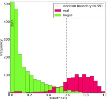
In our case, all three classifiers output a prediction or hypothe-sisfor each example. These hypotheses can be thought of as the probability a given example has of belonging to the class of real images, taking on values in the range 0–1. A classifier predicts de-tections with hypotheses close to 1 are highly likely real transients, while those close to 0 are bogus. In Fig. 5, we plot the distri-bution of hypothesis values for a RF withn_estimators=100,

max_features=25 andmin_samples_leaf=1 trained on four folds of the training set. The distribution plotted shows the hypothe-ses for the held-out fifth fold. To assign a label of real or bogus, we must define a decision boundary: a hypothesis value above which the classifier labels detections as real, otherwise detections are

la-Figure 5. Hypothesis distribution produced during one permutation of five-fold cross-validation. The hypotheses shown are for images in the held-out fold. Green shows the hypotheses for the validation examples labelled as artefacts and red those labelled as real. The decision boundary is selected such that the fraction of detections labelled as bogus lying above the decision boundary is 0.01. The FPR can be visualized as the fraction of green bars with a prediction greater than the decision boundary, the MDR is the fraction of red bars with predictions less than the decision boundary. The first interval has a frequency of 2376, but the plot is truncated for clarity.

Figure 6. An example of the cross-validation process for an RF with

max_features=25 andmin_samples_leaf=1.

belled bogus. If the classifier has learnt a useful model, it should output detections labelled as bogus with a hypothesis below the decision boundary and those labelled as real above the decision boundary for the prediction to be correct. Bogus detections with predictions above the decision boundary are false positives and real detections with hypotheses below the decision boundary are missed detections. For our FoM, the decision boundary is selected as the hy-pothesis value above which only 1 per cent of the bogus detections lie (dashed line in Fig.5). The FoM is the fraction of the detections labelled as real that lie below this choice of decision boundary. Dur-ing five-fold cross-validation a hypothesis distribution is generated by predicting hypotheses for the detections in each of the held-out folds.

In Fig. 6, we show an example of the five-fold cross-validation process for an RF with max_features=25 and

min_samples_leaf=1. In this example, we vary the number of decision trees,n_estimatorsand plot a receiver operator charac-teristic (ROC) curve for each model. ROC curves are produced by varying the decision boundary at which we assign a prediction to a label of real or bogus and calculate the FPR and MDR that deci-sion boundary produces for the validation set. From the example in Fig.6, we see that selecting a value of 100 forn_estimators pro-duces the best FoM of∼0.167, this means that an FPR=1 per cent produces an MDR of 16.7 per cent. We also include 5 and 10 per cent FPR levels for reference. We repeated this process for various sizes of hidden layer. We also show an example of measuring the FoM on a data set containing a significant proportion of the training data, labelled as overfit in Fig.6.

By replicating this process for both ANNs and SVMs, we were able to select the optimal set of hyperparameters for each algo-rithm. In the second column of Table2, we show the optimal hy-perparamters selected for each algorithm by cross-validation. By using the validation sets to select the hyperparameters, there is a danger that the hyperparameters will in effect have been fitted to these sets. As a result, the FoM we measure on the validation sets is not an unbiased measurement of the performance we would expect

(10)

Table 2. Comparison of learning algorithms.

Classifier Model parameters Threshold FoM

Artificial neural network s2=200,λ=5 0.547 0.233

Support vector machine (RBF) C=3,gamma=0.01 0.788 0.196

Random forest n_estimators=1000,max_features=25,min_samples_leaf=1 0.539 0.106

to achieve on data not included in the training folds. We deal with this in the next section.

4.4.2 Testing

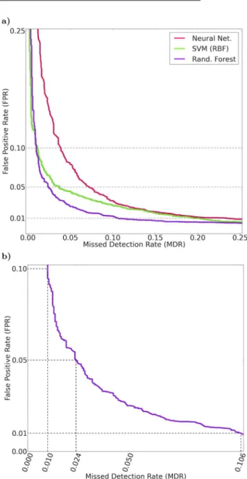
Having selected the optimal model for each of the algorithms, we retrain these models with the entire training set. This allows the models to learn from more examples. To measure how well we expect the models selected by cross-validation in the last section to perform on unseen data, we measure the FoM on the test set, the 25 per cent of the data we held back from both training and validation. This provides an unbiased estimate of the performance. In Table2, we show the FoM measured on the test set. Fig.7(a) shows the ROC curve for each model in Table2. We find that the RF is the best classifier with an FoM of 0.106.

Fig.7(b) shows a close-up of the measured FoM for the RF classi-fier, where the measured FoM is shown along with the performance we would expect to achieve if we were to allow 5 or 10 per cent of the bogus detections through to human scanners. For example, allowing the FPR to slip to 5 per cent increases the completeness to 97.6 per cent. We also plot the hypothesis distribution for the detections in the test set in Fig.8.

The FoM shown in Fig.7(b) is the single best classifier we find in our analysis. Using this classifier on a data stream of nightly obser-vations from PS1, we would expect that 99 per cent of the detections promoted to humans would be of real astrophysical transients while 10.6 per cent of the real detections would be rejected by the clas-sifier. Brink et al. (2013) report an MDR of 7.7 per cent for their system. As a next step, it is useful to investigate the detections for which the classifier produces incorrect predictions to see if there are systematic errors that the classifier makes or if it is making correct predictions for detections that have been labelled incorrectly during the construction of the training set.

5 F U RT H E R A N A LY S I S

In this section, we attempt to get a better sense of how we expect the classifier to perform in practice by characterizing its performance under various conditions. We aim to identify trends in the kinds of detections for which the classifier makes incorrect predictions and investigate the effect that providing the classifier with incorrectly labelled training and test sets has on the measured FoM. However, we begin this section by looking at methods to boost performance by combining classifiers.

5.1 Combining classifiers

As a last step towards boosting performance, we investigated a selection of methods to combine the RF, SVM and ANN from Table2. The predictions of the three methods are correlated: a candidate highly ranked by the RF is likely to also be highly ranked by the other two classifiers, but there are still detections of real transients that are discarded by only one of the classifiers. From Fig. 9there are 24 detections labelled as real that only the RF

Figure 7. (a) Comparison of the best models for various learning algorithms applied to the held-out test set. (b) Detail of ROC curve of the best performing classifier, the RF shown in (a). At an FPR of 1 per cent, the FoM shows that in practice we expect to operate at an MDR of 10.6 per cent.

wrongly rejects, it is these examples that we hope to recover by combining classifiers.

We tried only a few of the simplest combination strategies. First, we simply classified a detection based on the majority vote of the three classifiers. Secondly, we assigned each detection a hypothesis that was the mean of the hypothesis values output by each classifier. This produced a new distribution of mean hypotheses, where we again selected the decision boundary to produce the FoM. Finally

(11)

Figure 8. Hypothesis distribution for the optimal RF classifier applied to the test set.

Figure 9. Venn diagram showing the relationship between the missed de-tections for each classifier. There are 1619 positive examples in the test set.

Table 3. Results of combining classifiers.

Method FPR MDR

Majority vote 0.02 0.06 Mean hypotheses 0.01 0.12 Hypotheses as features 0.01 0.12

we trained an SVM using the three hypotheses for each detection as the features representing that detection. In the end, none of these methods outperformed the RF classifier, though the performance was comparable (see Table3).

This result is unsurprising given that the classifiers are highly correlated and there is no guarantee that these methods will outper-form the best individual classifier (Fumera & Roli2005). The RF is in itself an ensemble of classifiers (the individual decision trees)

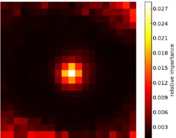
Figure 10. The relative importance of each pixel to the classification for the RF. The contributions of each feature are normalized such that they sum to 1.

and may already incorporate much of the gain in performance we can expect from these simple methods.

5.2 Relative feature importance

RFs provide a built-in method to estimate the relative importance of each feature to the classification (Breiman2001). By inspecting the ‘depth’ at which each feature is used as a decision node, we can estimate the relative importance of that feature, as those features used closer to the top of the tree will contribute to the prediction of a larger fraction of the training examples. The fraction of samples for which we expect a feature to contribute to the classification can be used to gauge its relative importance.

Fig.10shows the relative importance of each pixel determined from the training set. The relative importance metric is normalized such that it sums to 1. The most important features have the highest values and as would be expected are located in the centre of the image. The pixels on the edges of the images are thought to be important for identifying many of the bogus examples, where the object is not centred in the substamp and often lies at the edge. For reference if features were equally important, they would each have a relative importance of 1/400=0.0025.

Fig.10may suggest some redundancy in the features bounding the central pixels. It is expected that omitting these features would have little effect on the performance of our classifier as RFs are thought to be unaffected by the inclusion of noise variables in the feature vector (Biau2010). In contrast, Brink et al. (2013) find that the MDR for their RF classifier improves by∼4 per cent by omitting noisy features using a backward feature selection method. The effect of feature selection is an interesting area for future work and attempts at optimization.

5.3 Label contamination

We took care to eliminate label contamination in Section 3.1, by visually checking and manually labelling each training example. None the less we expect that there remain some examples with in-correct labels. In this section, we employ similar methods to those in Brink et al. (2013) to investigate the effect that label contamination has on our ability to train and test the optimal RF model.

(12)

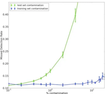
Figure 11. The effect of randomly flipping labels. As we increase the fraction of the images for which we flip the label, i.e. as we introduce more label contamination, the performance of the classifier trained on the contaminated training set and measured on the untouched test set (blue line) decreases as expected. Introducing contamination into the test set has a much more pronounced effect on the measured performance even at low fractions (green line).

First, we investigate the effect of adding label contamination to the training set. We add contamination by randomly selecting a subset of the detections from the training set and flipping their labels. Those labelled as real are now labelled as bogus and vice versa. In Fig.11, we plot the effect of randomly flipping labels in the training set while leaving the original labels in the test set untouched. The measured MDR appears fairly unaffected up to around 6 per cent contamination. The approach of Brink et al. (2013) is robust to around 10 per cent suggesting our method may be more susceptible to incorrectly labelled training data.

Next, we flip labels in the test set, while using the original training set labels as they are. Given that the RF has been trained with correctly labelled data, for the most part we expect it to provide the correct labels for the images in the test set. However, the flipped labels affect our ability to accurately measure the FoM. Although the classifier makes sensible predictions, when we compare these predictions to the flipped labels the otherwise correct predictions are now evaluated as false positives or missed detections. Fig.11

shows how the FoM is affected as we increase the fraction of flipped labels, we see that even at low proportions labelling noise in the test set can have a significant effect.

5.4 Classification as a function of signal to noise

To investigate the classifier performance as a function of S/N, we also follow a similar analysis to Brink et al. (2013). We plot the dis-tribution of magnitudes for each example in the test set labelled as real in Fig.12. We divide the examples into 11 bins, each spanning 1 mag in the range 13–24 mag. We then use the classifier to make a prediction for the examples in each bin and calculate the fraction of examples classified as bogus which we take as an estimate of the classifier performance for objects at that level of S/N. For objects with magnitudes20 there is an∼6 per cent chance of missing real detections. Counterintuitively, the detection performance

deterio-Figure 12. Histogram of magnitudes for the test set examples labelled as real. We also show the MDR as a function of S/N which increases dramatically for sources brighter than magnitude 20.

rates for higher S/N objects. The number of examples of these cases are low as typically these objects result in artefacts from saturation and subsequent masking or unclean subtractions. However, this can also be understood as an effect of our feature representation, where we are learning classifications based on the relative intensity of pixels across the substamp. The tendency to misclassify such detec-tions could stem from a combination of the large relative intensity differences between pixels in these substamps that often charac-terize artefacts and the low numbers of high S/N images of real transients. This explanation is further supported by both the ANN and SVM, which also misclassify these objects, suggesting that the issue is with the data and not a consequence of the realization of the RF. In the next section, we try to identify any relationships in the missed detections.

5.5 Missed detections

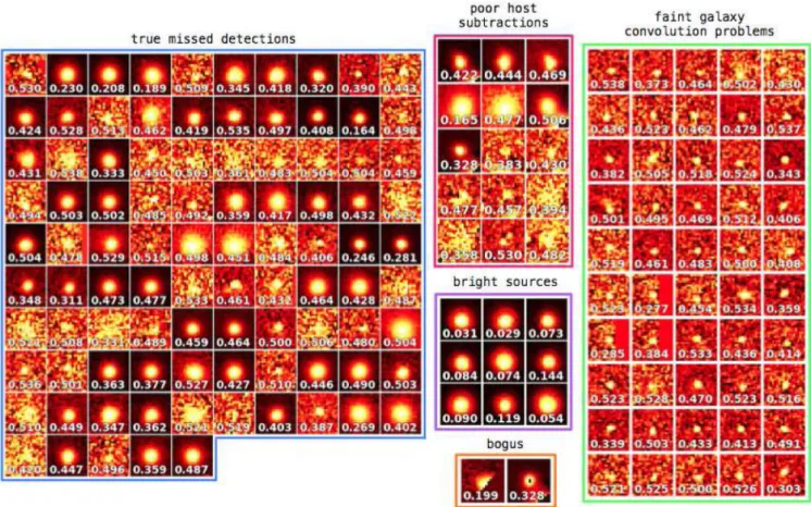
We inspected the 172 missed detections (see Fig.13) looking for similarities that may explain why they were rejected. We found that these missed detections are associated with 112 individual tran-sients. Although we took care to limit label contamination during the construction of the training set, we identified some examples of obvious bogus detections mislabelled as real that account for a small fraction (∼1 per cent) of the missed detections.

We also find about 29 per cent of the missed detections appear to be a result of faint galaxy convolution problems (see Section 2.1). These artefacts are difficult to identify by eye and as a result have been incorrectly labelled as real detections significantly contributing to the label contamination of the test set.

In Section 5.4, we discussed the high MDRs for bright sources. In Fig.14, we plot the hypothesis values for all detections included in the histogram of Fig.12(i.e. all test set detections that have been visually classified as real) against their magnitude reported by IPP. A feature of the plot that stands out is the cluster of sources with magnitudes brighter than 16 and hypotheses less than 0.2. Magnier et al. (2013) report that for the PS1 3π survey, saturation occurs at∼13.5 forgP1, rP1, iP1,∼13.0 forzP1 and ∼12.0 inyP1. We

were concerned that these sources could be saturated; however, to conclusively determine this the individual images that are combined to make a nightly stack would need to be examined. Instead, we

(13)

Figure 13. The 172 detections labelled as real but classified as bogus by the RF. Detections are grouped according to the discussion in Section 5.5. The hypotheses for the detections are shown as the inset numbers.

Figure 14. Plot showing the hypotheses of the real examples in the test set against the magnitude measured by IPP. The shaded region shows the magnitude cut above which we cannot be certain the nightly stacks do not contain saturated images.

scaled the magnitudes reported by Magnier et al. (2013) for PS1 3πexposures by the exposure times for the individual images that make up a nightly stack and set a magnitude limit of 16 mag. Objects brighter than this limit may have saturated cores in some exposures

and cannot safely be labelled as real. Some of these sources on close inspection also show signs of the unclean subtractions we highlighted in Section 2.1.

The detections brighter than 16 mag in Fig.14with hypotheses above 0.2 are all associated with a single confirmed SN, SN 2014bc (PS1-14xz; Smartt et al.2014). SN 2014bc is a nearby (7.6 Mpc) Type-IIP located in the bright host galaxy NGC4258 (Messier 106). The transient lies close to the core of the host and as a consequence the host has been poorly subtracted in the same location in all the substamps. Detections of this object appear in both the training and test set and although we ensured detections from the same night must appear in the same set, the slowly evolving plateau has resulted in detections with similar S/N and the same pattern of poor subtraction appearing in both. It is therefore to be suspected that test set detections associated with this SN would have been rejected along with the other sources brighter than 16 mag had similar detections not been included in the training set. This raises the issue of potentially missing the brightest transients which are often of interest and the cheapest to classify spectroscopically, we return to this in Section 6.

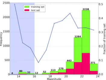
The high MDRs in the magnitude range 16–20 still remain unex-plained. To address this in Fig.15, we plot the number of examples of real transients in each of the magnitude bins used in Section 5.4 for both the training and test sets. The plot clearly shows the deficit in training examples at magnitudes brighter than 20 and lead us to conclude that we lack enough training examples of high S/N transients to allow the classifier to learn a model that generalizes well in this regime. In Fig.15, we overlay the relative size of the test set compared with the training set in each bin. We selected the

(14)

Figure 15. The magnitude distributions of the real examples in the training and test sets. The numbers on each bin show the total number of images in the training set. We also show the relative numbers of test set examples in each bin (blue line). The shaded region again shows the magnitude cut defined in Section 5.5.

test set by randomly sampling 25 per cent of the data available for training. The small fractions of test examples available between 16 and 18 mag combined with the low numbers in the range 16–20 mag severely impact our ability to accurately measure the MDR in this range.

Aside from the issues associated with high S/N, there are a few other SNe with detections that show similar host galaxy subtraction problems to SN 2014bc. Some of these are true bogus detections which we show in Fig.13. Approximately 9 per cent of the missed detections are bogus detections around poor host subtractions. We include detections of SN 2014bc with this group in Fig.13though these detections around 15th magnitude could equally have been included with the bright sources.

Among the missed detections, we also found substamps where entire rows or columns along an edge of a substamp had been masked. In the second panel of Fig.3, we show an example where the bottom two rows of pixels have been masked. These are examples of the sky cell duplicates we describe in Section 2.1. We were concerned that the classifier was rejecting these detections based on the masking. To see if this was the case, we identified all the examples of sky cell overlap among the real test set detections, and found 20. As we ensured that detections from the same night must be in the same set (training or test set), the equivalent full 20×20 pixel substamps were also in the test set. We compared the performance on the full pixel substamp with that of the partially masked substamp and found that there is only one case where the masked substamp was rejected while the full pixel substamp was kept. In this instance, a significant proportion of the substamp was masked (seven columns) with the edge lying close to the PSF. The majority of the remaining substamp pairs were both assigned the same classification. There are however six pairs where the masked substamp was correctly classified as real, but the full pixel substamp was rejected, showing that the classifier does not tend to reject detections with sky cell masking simply due to the masked regions. The reason for rejecting one detection from the pair over the other is unclear as both substamps are constructed from the same data. The six pairs for which the full pixel substamp was labelled bogus, but the masked substamp was labelled real are all associated with a single transient and may not apply to other sky cell pairs. For

these substamp pairs, we found that the centroids always differed by 1 pixel and were offset in the same direction. We tried shifting the centre of the stamps to the same pixel, but found that this had little impact on the hypothesis. In all cases, the flux-conserving warping results in equivalent pixels containing different counts, though the difference is typically small 10 per cent. Given the small number of cases where the detections of a sky cell pair are assigned to different classes (seven in total) and that these detections are associated with only two transients (six associated with a single transient where the full pixel substamp is rejected and one associated with a different transient where the masked substamp is rejected), it is difficult to explain this behaviour, though one explanation may be the small differences in pixel intensity values perhaps combined with the different centroids.

The nuances of difference imaging make it difficult to determine the ground truth label for each detection. Humans often require ad-ditional information beyond that contained in the single difference image e.g. position relative to the host, or the number of bad/good pixels visible in the input image. The investigations above suggest that the classifier is identifying subtle relationships and correctly identifying that many of the ‘missed detections’ are dubiously labelled as real. We estimate that 45 per cent (∼5 per cent bright sources;∼29 per cent convolution problems;∼9 per cent poor host subtractions;∼1 per cent obvious mislabelled artefacts) or about 77 of the missed detections are not of high enough quality to be confidently labelled as real detections. Therefore, the RF classifier is not strictly getting them wrong. The high proportions of these cases among the missed detections does not hold true for the entire sample of real detections in the test set, where for example faint galaxy convolution problems are crudely estimated to account for no more than 7 per cent. Removing such detections from our test set results in an MDR around 6.2 per cent. The MDR of our classifier is therefore in the range 6.2–10.6 per cent for an FPR of 1 per cent but most likely towards the lower end of this range. The remaining 95 detections are true missed detections and appear to be mislabelled by the classifier due to high S/N as discussed above, poor seeing conditions and very low S/N detections near the detection limit.

5.6 Medium deep confirmed SNe

In order to demonstrate how we might expect the classifier to per-form on a live data stream, we first use the classifier to make pre-dictions for the9_{PS1-13avb for which we held out all associated}

detections from both the test and training set. This object has been spectroscopically classified as a Type Ib SN and has a well sam-pled light curve from about−18 d pre-maximum to around 106 d post-maximum, including exposures in all five filters ranging in magnitude from around 23 to 20 mag (see Fig.16top panel). We selected this object for its high-quality light curve and magnitude range which represents the majority of objects discovered in the PS1 MDS. In the bottom panel of Fig.16, we show the hypothesis for each epoch of this target. The plot shows that the hypothesis is consistently above the decision boundary of 0.539 (selected in Sec-tion 4.4.2) with the excepSec-tion of the detecSec-tion from 56480.406 MJD which shows the transient at a magnitude ofgP1=23.12±0.21

approaching the detection limit in this filter. The detection is dis-played as an inset in Fig.16with its hypothesis of 0.506, showing the low S/N and deviation from a PSF-like morphology.

9_supernova

(15)

Figure 16. Top panel: PS1 light curve of the Type Ib SN PS1-13avb. Bottom panel: the hypothesis for each epoch. The dashed line shows the decision boundary (0.539) below which the classifier predicts an image as bogus. Inset: the only missed detection for this SN which shows low S/N.

5.7 Early detection

One of the major aims of recent SN searches has been to try to detect the transient as soon after explosion as possible in order to trigger rapid follow-up to spectroscopically study regions of the transients evolution that remain relatively unexplored (Cao et al.2013; Gal-Yam et al.2014). To this end, we carry out a simple test by using the classifier to make predictions for the first detections of all 53 classified SNe in our data base. Again we held these detections out from the training and test sets. In Table4, we list the 53 SNe and the details of the first detections along with the hypothesis for each detection. The classifier correctly predicts all detections as real and had it been running on a live data stream would have promoted all objects to humans for follow-up.

6 S U M M A RY O F R E S U LT S A N D C O N C L U S I O N S

In this work, we have constructed a data set of detections from the PS1 MDS. We used this data set to train an RF classifier to reject bogus detections of transients before they are presented to humans as potential targets for follow-up. As the feature representation of these detections, we used the pixel intensity values of a 20×20 pixel substamp centred on the detection. This choice is independent of the observing strategy and removes the need for careful feature design and selection that requires specific domain knowledge. The choice of features also make this method applicable to any survey performing difference imaging and requires no information from either the template image or nightly stack. Using the FoM as defined in Brink et al. (2013), we selected the decision boundary such that

objects classified as real should be 99 per cent pure, which resulted in a best estimate of an MDR of 6.2 per cent (i.e. 93.8 per cent complete) and can compete with previous work in this area. We further tested the classifier by applying it to the light curve of a Type-Ib SN and found only one missed detection out of 74. The missed detection had low S/N. In addition, to assess the classifiers performance for early detection, we used the classifier to make predictions for the first detections of 53 spectroscopically confirmed SNe in our data base and found none would have been rejected.

We discovered our classifier struggles to provide accurate clas-sifications for the brightest sources (<19 mag). Many of these are associated with bright variable stars and have ringing patterns due to the kernel size definition, which leads to labelling difficulties. Some are also close to the saturation limit which may cause the algorithms to misidentify real sources as bogus. The mathematical problem in detecting bright variable stars in difference images is clearly quite distinct from finding low flux and moderate flux level transients in, or near extended galaxies. Furthermore, the scientific goal in characterizing variability of stellar sources is typically based on total flux measurements whereas finding explosive transients re-quires the resolved and unresolved galaxies to be subtracted. Our methods are tailored towards the latter, and can certainly not be blindly applied to uncover complete populations of variable stars or variable AGNs. With a goal of discovering extragalactic transients, one is content to ignore stellar variables in a data stream, although we show here that the algorithms can sometimes misclassify bright and high S/N explosive transients.

We also found the MDR is consistently higher for sources brighter than 20 mag which we attribute to the lack of training data in this range. We would expect that providing more training examples that are representative of these objects would reduce the MDR for brighter sources. In this paper, we have only used a sample of the data from the PS1 MDS, but we have access to the full data base of MDS transients, which could be used to provide more training data. In addition, we also have data from PS1 3πdifference imaging which could also be used to boost training numbers and build a classifier that could perform real–bogus classification for both surveys. In our analysis, we have not considered the case of asteroids as these are typically removed during the construction of the nightly stacks in the MDS. Including the PS1 3π data, where differencing is performed on individual exposures, would allow us to test the performance of our method on asteroids. It may also be more beneficial to apply this approach at the source extraction stage. By working directly on the pixel data, the classifier could potentially learn which sources to extract and which to discard from a difference image before any further processing of a potential detection is performed.

The dependence of any machine learning approach to real–bogus classification on large amounts of training data presents a serious problem for any new survey. While many sources of processing arte-facts are common across surveys, differing pixel scales and seeing conditions prevent the use of a classifier trained on one survey being directly applied to another. A solution would be to build a training set based on hand labelled commissioning data and periodically re-train the classifier as new data become available. Alternatively, an initial classifier trained on the limited data available early in a sur-vey could be improved on by employing online learning, where the classifier is automatically updated as new labelled data are gathered (Saffari et al.2009; Shalev-Shwartz2011).

Future work will focus on combining the remaining PS1 data available into a single training set that will hopefully address the S/N issue. Other areas of research could include the use of

(16)

Table 4. First detections of the 53 spectroscopically confirmed PS1 SNe ordered by hypothesis. (Due to sky cells some SNe appear twice.)

Name Classification First detection (MJD) Magnitude Filter Hypothesis

PS1-13duq Ia 56588.381 21.64 iP1 0.989 PS1-13bzp Ia 56478.276 21.33 gP1 0.98 PS1-13bzp Ia 56478.276 21.30 gP1 0.975 PS1-13abg II-P 56383.336 21.47 zP1 0.971 PS1-13bqg Ia 56443.287 20.90 gP1 0.968 PS1-13abg II-P 56383.336 21.55 zP1 0.963 PS1-14il IIn 56676.554 21.36 zP1 0.959 PS1-13vc Ia 56351.476 20.67 zP1 0.958 PS1-13abw Ic 56383.438 21.23 zP1 0.958 PS1-14ky II 56681.499 21.60 zP1 0.957 PS1-13ur Ia 56351.525 20.32 zP1 0.955 PS1-13eae II 56604.598 19.82 yP1 0.954 PS1-13alz II-P 56399.282 20.43 iP1 0.952 PS1-12cnr Ia 56283.340 20.33 zP1 0.948 PS1-13can Ia 56477.567 22.04 zP1 0.946 PS1-13cws Ia 56549.460 21.48 zP1 0.943 PS1-13ge Ia 56328.612 21.49 gP1 0.94 PS1-12cho Ia 56262.469 21.07 zP1 0.933 PS1-12cey II 56268.294 22.06 gP1 0.931 PS1-13bok I 56424.560 22.35 rP1 0.926 PS1-13djz Ic 56554.585 20.74 zP1 0.923 PS1-13a Ia 56289.280 21.20 zP1 0.919 PS1-13bit Ia 56420.548 22.69 iP1 0.918 PS1-13bqb Ia 56443.287 22.32 gP1 0.918 PS1-13djj Ia 56563.576 20.72 gP1 0.916 PS1-12bza II-P 56262.469 21.12 zP1 0.914 PS1-13brf Ia 56443.324 22.68 rP1 0.91 PS1-13hp II-P 56325.545 21.40 gP1 0.907 PS1-13adg Ia 56384.515 21.71 rP1 0.902 PS1-13awf I 56417.315 22.47 iP1 0.899 PS1-13atm II-P 56410.298 22.25 zP1 0.898 PS1-13cjb II 56501.436 22.63 gP1 0.896 PS1-12cho Ia 56262.469 21.08 zP1 0.884 PS1-13cai Ia 56477.567 21.99 zP1 0.882 PS1-13bni II-P 56420.548 23.07 iP1 0.873 PS1-13bog Ia 56417.341 22.57 iP1 0.867 PS1-12chw Ia 56262.313 21.21 yP1 0.857 PS1-13bqv Ia 56442.486 21.64 zP1 0.849 PS1-13djs Ia 56562.587 21.44 zP1 0.84 PS1-13aai/SN 2013au Ia 56370.421 19.29 zP1 0.833 PS1-13cuc/SN 2013go Ia 56536.587 19.03 zP1 0.814 PS1-13hs I 56328.515 21.97 gP1 0.801 PS1-13baf II-P 56414.521 22.54 iP1 0.801 PS1-13avb Ib 56414.521 21.75 iP1 0.796 PS1-13ayn Ia 56416.449 22.01 rP1 0.77 PS1-13aai/SN 2013au Ia 56370.421 19.36 zP1 0.735 PS1-13fo/SN 2013X Ia 56314.625 18.04 yP1 0.713 PS1-13bus Ia 56462.440 22.91 iP1 0.708 PS1-13brw II-P 56436.325 20.71 yP1 0.707 PS1-13hi IIn 56324.604 18.50 zP1 0.704 PS1-13bvc Ia 56469.349 21.90 zP1 0.698 PS1-13bzk Ia 56468.571 21.38 yP1 0.662 PS1-13abf Ia 56380.368 20.21 yP1 0.642 PS1-13arv Ia 56409.239 20.98 yP1 0.638 PS1-13wr II-P 56349.602 20.39 yP1 0.637 PS1-14xz/SN 2014bc II-P 56399.380 18.25 iP1 0.623 PS1-13wr II-P 56349.602 20.40 yP1 0.61 PS1-13buf Ia 56461.299 22.60 zP1 0.577