Continuous Statistical Models:
With or Without Truncation Parameters?
V. Vancak1*, Y. Goldberg1**, S. K. Bar-Lev1***, and B. Boukai2**** 1Dept. Statist., Univ. Haifa, Israel
2Dept. Math. Sci., IUPUI, ??????
Received June 29, 2014; infinal form, February 10, 2015
Abstract—Lifetime data are usually assumed to stem from a continuous distribution supported on[0, b) for someb≤ ∞. The continuity assumption implies that the support of the distribution does not have atom points, particularly not at 0. Accordingly, it seems reasonable that with an accurate measurement tool all data observations will be positive. This suggests that the true support may be truncated from the left. In this work we investigate the effects of adding a left truncation parameter to a continuous lifetime data statistical model. We consider two main settings: right truncation parametric models with possible left truncation, and exponential family models with possible left truncation. We analyze the performance of some optimal estimators constructed under the assumption of no left truncation when left truncation is present, and vice versa. We investigate both asymptotic andfinite-sample behavior of the estimators. We show that when left truncation is not assumed but is, in fact present, the estimators have a constant bias term, and therefore will result in inaccurate and inefficient estimation. We also show that assuming left truncation where actually there is none, typically does not result in substantial inefficiency, and some estimators in this case are asymptotically unbiased and efficient.
Keywords:truncation parameter, estimation, order statistics, efficiency, model selection. 2000 Mathematics Subject Classification:????
DOI:10.3103/S1066530715010019
1. INTRODUCTION
When modeling lifetime data it is usually assumed that the distribution is continuous and supported on Ω1 = [0, b), b≤ ∞. Here b is either a known constant or a parameter (Elandt-Johnson, 1999;
Lawless, 2003). However, is this the right support? The continuity assumption implies that the support
Ω1 of the distribution does not have atom points, particularly not at 0. Thus one can expect that all
observations will be positive. Indeed, when the lifetime data measure time to events such as death or remission, it seems reasonable to assume that one observes only positive time to event values. Even when the observed data is on events of small time scale (such as time of detection of motion sensors), as measured with an accurate measuring tool, it is expected that all observations would be positive. This suggests that the true support may be truncated from the left and is, in fact, of the formΩ2 = [γ, b),
γ >0, withγunknown.
In this work we consider models that allow the support of the distribution to be chosen adaptively from the data by using truncation parameters. Each of these proposed models can be considered as generalization of a model in which the support includes{0}. A natural question that arises is which of these two models should we use? With this, we need to consider two possible errors. To describe these errors, let Model I denote the statistical model of which the true support isΩ1= [0, b), and let Model II
denote the truncated statistical model of which the true support isΩ2= [γ, b), γ >0. We say that a False
* E-mail:??? **E-mail:[email protected] ***E-mail: ???? **** E-mail:????? 1
This is the author's manuscript of the article published in final edited form as:
Vancak, V., Goldberg, Y., Bar-Lev, S. K., & Boukai, B. (2015). Continuous statistical models: With or without
truncation parameters?. Mathematical Methods of Statistics, 24(1), 55-73.
Model I error has occurred if Model I has been incorrectly used for inference while the correct model is Model II. A False Model II error is defined similarly. Then the question arises: Which of the two types of errors is more severe? The answer to this question is useful when the model’s underlying true support is unknown.
It seems reasonable that even ifΩ1 = [0, b)is the correct support, using Model II will not result in
substantial loss of information. Conversely, ifΩ2 = [γ, b)for someγ >0is the correct support, there will
be substantial loss of information when using Model I. This claim can be justified in terms of sufficiency. Assume that Model I depends on some unknown parameterθ(possibly a vector), and is associated with a minimal sufficient statistictn=t(Xn). Model II, which is obtained by a left-truncation of Model I, is therefore parameterized byη= (γ, θ)and is associated with the minimal sufficient statistic(X(1), tn). Note that (X(1), tn), while being a minimal and sufficient statistic for Model II, is still sufficient for
Model I; whereastnalone, while being minimal and sufficient for Model I, is not sufficient for Model II, hence we expect the False Model I error to be more critical. As we later show, this understanding, while essentially correct, requires some further clarifications.
Two main settings are investigated in this work. In thefirst one, we assume that the density function is known up to a right truncation parameter. In this setting, under Model I, there is only a right truncation parameterθ. In other words,Ω1 = [0, θ). Under Model II, we assume also left truncation and hence the
support isΩ2= [γ, θ). For this setting, two candidate estimators (Tate, 1959; Bar-Lev and Boukai 1985)
will be compared for their cross-model bias and MSE, as well as for their asymptotic efficiency. More specifically, for the right truncation setting with a possible left truncation parameter, we are interested in the behavior of the Bar-Lev and Boukai (1985) (hereafter abbreviated BB) estimator when there is no left truncation, and the behavior of the Tate’s estimator (Tate, 1959) when left truncation is indeed present.
The second setting deals with distributions having a ‘regular’ parameter with a possible left trunca-tion. We begin with the Erlang distribution as a special case of the natural exponential family (NEF), and illustrate the effect of the possible truncation on the estimator of the ‘regular’ parameter. We proceed to discuss this problem in the general case of the NEF distribution, however in the asymptotic sense only.
The question discussed in this paper can be considered as a model selection problem. One can think about Model I as a narrow model and on Model II as a wider model since Model II includes an additional parameter. Selecting the right model was addressed considerably in the literature for maximum likelihood estimation, and in particular for linear regression, using tools such as AIC and BIC (see, for example, Burnham and Anderson, 2002). The consequences of choosing a misspecified model when using maximum likelihood estimation were discussed by White (1982), among others. Bickel (1984) considered the effect of misspecification for linear regression model. Claeskens and Hjort (2008) suggested criteria, such as tolerance radius, for choosing between a narrow model and a ’wider’ one. We note that since the two possible models we consider have different supports, many of the results mentioned above do not hold for this setting (see, for example, White (1982), Assumption A7). Moreover, the approach we consider here, at least for thefirst setting, does not fall under the maximum likelihood estimation. Finally, most of our analysis is exact and not asymptotic. Hence, this paper offers a new approach for an interesting novel problem of model selection.
The paper is organized as follows. The analysis of continuous statistical right-truncated models with possible left truncation is presented in Section 2. In Section 3 we discuss in detail the Erlang distribution case, and conclude with some asymptotic aspects of possible truncation in the NEF case. Concluding remarks appear in Section 4. The proofs are presented in the Appendix.
2. RIGHT TRUNCATED MODELS WITH A POSSIBLE LEFT TRUNCATION
In Section 2.1 we present the model. We then discuss estimation in Section 2.2, and cross-model analysis in Section 2.3. Finally, in Section 2.4, we illustrate the results by examples.
2.1. General Setup
Leth(·)be a positive integrable function over[0,∞). For any0≤γ < θwe define gk(γ, θ) =
∫ θ
γ
xkh(x)dx, k= 0,1,2, . . . . (1)
Using (1), we construct the probability density function (p.d.f.) of a continuous type random variableX as
f(x;η) = h(x)
g0(γ, θ)
I[γ < x < θ]. (2)
Here,I[A]is the indicator function of the setAandγandθare the two possibly unknown parameters of f(x;η). Accordingly, we consider two possible models forη≡(γ , θ):
• Model I: γ ≡γ0= 0 is known, while θ > γ0 is an unknown parameter, so that η0 ≡(γ0, θ)
designates the model’s only unknown parameterθ.
• Model II: Both γ and θare unknown parameters, 0< γ < θ, so thatη≡(γ , θ) designates the model’s two unknown parameters.
Note that with the notation in (1), the moments ofXunderηare easily defined by Eη(Xk) = gk(γ, θ)
g0(γ, θ)
, k= 0,1,2, . . . . (3)
In particular, the expected value ofXisEη(X) =g1(γ, θ)/g0(γ, θ). Similarly, the cumulative
distribu-tion funcdistribu-tion (c.d.f.) ofXis given, for anyτ ∈R, by Fη(τ)≡Pη(X≤τ) =
g0(γ, τ)
g0(γ, θ)
I[γ < τ < θ] +I[θ≤τ], (4) with the corresponding tail probability
1−Fη(τ)≡Pη(X > τ) =I[τ ≤γ] + g0(τ, θ)
g0(γ, θ)
I[γ < τ < θ]. (5)
Following (4), the π-th quantile is given byτπ that solves the equation Fη(τπ)≡P(X≤τπ) =π for γ < τπ < θ, and can be expressed using the inverse of the cumulative distribution function
τπ =Fη−1(π), (6)
such thatπ ≡Fτ(τ) =g0(γ, τ)/g0(γ, θ).
As before, letXn= (X1, X2, . . . , Xn)be a sample ofni.i.d. observations fromf(x;η)in (2), and let
X(1)≤X(2) ≤ · · · ≤X(n) denote the corresponding order statistics. It is a standard exercise to show
that under Model I, the minimal sufficient statistic (MSS) for η0≡(0, θ) is SI =X(n), while under
Model II, withη≡(γ, θ), the MSS isSII = (X(1), X(n)). Under Model I, the p.d.f. of the MSS statistic
SI =X(n)is fSI(t;η0) = nh(t)(g0(0, t) )n−1 ( g0(0, θ) )n I[0< t < θ], (7)
whereas, under Model II, the p.d.f. ofSII = (X(1), X(n))can be shown to be
fSII(y, t;η) = n(n−1)h(y)h(t)(g0(y, t) )n−2 ( g0(γ, θ) )n I[γ < y < t < θ]. (8) We finally note that under Model I, when η ≡η0 = (0, θ), the statistic SII = (X(1), X(n)), while
sufficient forθ, is not minimal, and its p.d.f. is given by fSII(y, t;η0) = n(n−1)h(y)h(t)(g0(y, t) )n−2 ( g0(0, θ) )n I[0≤y < t < θ]. (9)
However, under Model II,η≡(γ, θ), and the statisticSI =X(n)is not sufficient for the unknownη, and its p.d.f. is given by fSI(t;η) = n h(t)(g0(γ, t) )n−1 ( g0(γ, θ) )n I[γ ≤t < θ].
Regardless of the assumed model (Model I or II), it is easy to verify that the conditional p.d.f. ofX(n)
givenX(1)=y(withy > γ) is given by
fX(n)|X(1)(t;y, θ) = (n−1)h(t)(g0(y, t) )n−2 ( g0(y, θ) )n−1 I[y < t < θ], (10)
whereas the marginal p.d.f. ofX(1)is fX(1)(y;η) = n h(y)(g0(y, θ) )n−1 ( g0(γ, θ) )n I[γ < y < θ]. (11) 2.2. UMVU Estimation
Letξ(η)be any estimable function of the model’s unknown parameterη. For instance,ξ(η) =Eη(X), orξ(η) =Fη(τ), for somefixedτ ∈R. Based on the sample datax= (x1, x2, . . . , xn), we are interested in constructing a UMVUEξˆn≡ξˆ(S(x))forξ(η). Clearly, for anyη, this estimator should satisfy
Eη( ˆξn) =ξ(η). (12)
By repeatedly differentiating both sides of (12) with respect to the components of η, along with application of Leibniz’s integral rule, one can obtain (in the case of distributions of the form in (2)), explicit expressions for such UMVU estimators.
Tate (1959) considered this problem under Model I (i.e., η≡η0 = (0, θ) and SI(x) =x(n)) and
obtained that the general form of the UMVUE forξ(θ)is
ˆ ξIn=ξ(x(n)) +ξ ′(x (n))g0(0, x(n)) nh(x(n)) (13) whenever the derivativeξ′(θ) =∂ξ(θ)/∂θ exists and is continuous almost everywhere on the support
Ω1 ={(0, θ) :a < θ < b}.
Similarly, Bar-Lev and Boukai (1985) considered the same estimation problem under Model II (i.e.,η≡(γ, θ)andSII(x) = (x(1), x(n))). They showed that the general form of the UMVUE for any
estimable functionξ(γ, θ)is ˆ ξnII =ξ(x(1), x(n))− g0(x(1), x(n))ξ1(x(1), x(n)) (n−1)h(x(1)) +g0(x(1), x(n))ξ2(x(1), x(n)) (n−1)h(x(n)) − g20(x(1), x(n))ξ12(x(1), x(n)) n(n−1)h(x(1))h(x(n)) , (14)
whenever the partial derivativesξ1 =∂ξ/∂γ,ξ2=∂ξ/∂θ, andξ12=∂2ξ/∂γ∂θexist and are continuous
almost everywhere onΩ2={(γ, θ) :a < γ < θ < b}.
Remark 1. Assume that Model II holds, butξ(γ, θ)≡ξ(θ)for some estimable function ofθalone. Then, similarly to (13), the general form of the BB’s UMVUE forξ(θ)is reduced to
ˆ ξnII =ξ(x(n)) +ξ ′(x (n))g0(x(1), x(n)) (n−1)h(x(n)) , (15)
where ξ′=∂ξ/∂θ. A comparison of ξˆnI in (13) to ξˆIIn in (15) reveals the extent of the bias upon erroneously using Tate’s estimatorξˆnIinstead of the UVMUEξˆnII. In fact, it can be easily seen that
ˆ ξnI = ˆξnII+ξ ′(x (n)) h(x(n)) (g 0(0, x(n)) n − g0(x(1), x(n)) n−1 ) ≡ξˆII n +bn.
Hence, since Eη( ˆξnII) =ξ(θ), it immediately follows that Eη( ˆξnI) =ξ(θ) +Bn, where Bn≡Eη(bn)
represents the bias.
Remark 2. It can be shown (see (10) and (11)) that under Model II, the conditional expectation ofξˆII n , givenX(1)=y, is
Eη( ˆξIIn |X(1) =y) =ξ(y, θ)−
ξ1(y, θ)g0(y, θ)
nh(y) ≡r(y, θ). (16)
Hence, by Remark 1 and (15),ξˆIIn must be of the form
ˆ
ξIIn (y, t) =r(y, t) +r2(y, t)g0(y, t)
(n−1)h(t) , (17)
wherer2 =∂r/∂θ.
In the next section we provide a more general assessment of the bias term in (15). Examples for Tate’s and for BB’s UMVU estimators are provided below; we omit the derivations.
Example 1. Under Model I:
(a) Forξ(θ) =Eη0(X
k) =gk(γ
0, θ)/g0(γ0, θ), with knownγ0 = 0, it can be shown that Tate’s UMVU
estimator is ˆ ξnI = gk(0, x(n)) g0(0, x(n)) ( 1− 1 n ) +x k (n) n .
(b) In particular, fork= 1, we have that ξ(θ) =Eη0(X) =g1(γ0, θ)/g0(γ0, θ), with knownγ0 = 0. It can be shown that Tate’s UMVU estimator is
ˆ ξnI = g1(0, x(n)) g0(0, x(n)) ( 1− 1 n ) +x(n) n .
(c) Forξ(θ) = 1−Fη0(τ) =g0(τ, θ)/g0(γ0, θ), with knownγ0 = 0, andτ ≥γ0, it can be shown that Tate’s UMVU estimator is
ˆ ξnI = 1− ( 1− 1 n ) g 0(0, τ) g0(0, x(n)) .
(d) For ξ(θ)≡τ =Fη−01(g0(γ0, τ)/g0(γ0, θ)), with known γ0= 0, and τ ≥γ0, it can be shown that
Tate’s UMVU estimator forτ is
ˆ ξIn=Fη−01 ( g0(0, τ) g0(0x(n)) ) + g 2 0 ( 0, Fη−01(x(n)) ) g0(0, x(n)) nh(x(n))g0(0, τ)h(Fη−01(x(n))) . (18)
Example 2. Under Model II:
(a) For ξ(θ) =Eη(Xk) =gk(γ, θ)/g0(γ, θ), with known γ >0, it can be shown that BB’s UMVU
estimator is ˆ ξnII = gk(x(1), x(n)) g0(x(1), x(n)) ( 1− 2 n ) +x k (1)+x k (n) n .
(b) In particular, for k= 1, if ξ(γ, θ) =Eη(X) =g1(γ, θ)/g0(γ, θ), the general form of BB’s UMVU estimator is ˆ ξnII = gk(x(1), x(n)) g0(x(1), x(n)) ( 1− 2 n ) +x(1)+x(n) n .
(c) Forξ(γ, θ) = 1−Fη(τ) =g0(τ, θ)/g0(γ, θ),γ ≤τ ≤θ, one obtains that BB’s UMVU estimator is
ˆ ξnII = ( 1− 1 n ) −(1− 2 n ) g0(x(1), τ) g0(x(1), x(n)) .
(d) It follows from (6) that forξ(θ) =Fη−1(g0(γ, τ)/g0(γ, θ)), withγ >0andτ ≥γ, BB’s UMVU is
ˆ ξnII =Fη−1 ( g0(x(1), τ) g0(x(1), x(n)) ) − g0(x(1), x(n))g02(Fη−1(x(1)), x(n)) (n−1)h(x(1))h(Fη−1(x(1)))g0(Fη−1(x(1)), τ) − g0(x(1), x(n))g02(x(1), Fη−1(x(n))) (n−1)h(x(n))h(Fη−1(x(n)))g0(x(1), τ) −g 2 0(x(1), x(n))ξ12(x(1), x(2)) n(n−1)h(x(1))h(x(n)) , where ξ12(x(1), x(n)) =− Fη12(Fη−1(x(1)), x(n)) (Fη1(Fη−1(x(1)), x(n)))2Fη2(Fη−1(x(1)), Fη−1(x(n))) ,
assuming that the partial derivativesFη1 =∂Fη/∂γ,Fη2 =∂Fη/∂θ, andFη12=∂2Fη/∂γ∂θexist and
are continuous almost everywhere onΩ2 ={(γ, θ) :a < γ < θ < b}.
2.3. Cross-Model Analysis
The analysis in this section focuses on model misspecification, where the quantities of interest are (i) the estimators’ expectations and (ii) the estimators’ MSE w.r.t. the incorrect support. In other words, what is the reduction in efficiency (if any) when we derive the estimators w.r.t. Model I support while actually Model II support holds, and vice versa. More specifically, we are interested in the evaluation of E( ˆξn|I Model II) =Eη( ˆξnI)whenη= (γ, θ)is the unknown parameter, and ofE( ˆξnII|Model I) =Eη0( ˆξ
II n ) whenη0 = (0, θ)andθis the only unknown parameter. Similar cross-evaluations will be considered for
theM SE( ˆξn|I Model II) =Eη(( ˆξnI−ξ)2)and theM SE( ˆξnII|Model I) =Eη0(( ˆξ
II
n −ξ)2). In the follow-ing theorem we evaluate the extent of the cross-model bias by straightforward calculations.
Theorem 1. Let ξ(η) be any estimable function, i.e., any function of the unknown parameters
which possesses an unbiased estimator under both ModelIand ModelII (e.g., Examples1, 2), and letξˆInandξˆnIIbe its respective estimators.
(i) Under False ModelImisspecification we have
E( ˆξn|I Model II) =Eη( ˆξnI) =ξ(θ)(1 +a) +bn, (19) where, withη= (γ, θ),a=g0(0, γ)/g0(γ, θ)and
bn=−a ∫ θ γ ξ(t)(n−1)h(t)(g0(γ, t)) n−2 (g0(γ, θ))n−1 dt .
(ii) Under False ModelIImisspecification we have E( ˆξIIn |Model I) =ξ(η) +d1n+d2n, where d1n≡Eη0( ˆξ II n I[0< y < t < γ]) = ∫ γ 0 ∫ t 0 ˆ ξnII(y, t)fSII(y, t;η0)dy dt and d2n≡Eη0( ˆξ II n I[0< y < γ < t < θ]) = ∫ θ γ ∫ γ 0 ˆ ξnII(y, t)fSII(y, t;η0)dy dt .
The proof appears in Appendix A1.
Note that since ξˆnI and ξˆnII are UMVUE for ξ(θ) and ξ(η), respectively, under the correct models, it holds that Eη( ˆξnII) =ξ(η), M SE( ˆξnII|Model II) = Varη( ˆξnII), and Eη0( ˆξ
I
n) =ξ(θ), with M SE( ˆξn|I Model I) = Varη0( ˆξ
I
n). Further, since by part (i) of Theorem 1, ξˆnI is a biased estimator of ξ(η)≡ξ(θ)under Model II, it follows immediately that it is an inconsistent estimator and that
M SE( ˆξnI|Model II) = Varη( ˆξnI) + (ξ(θ)a+bn)2 > M SE( ˆξnII|Model II).
Proposition 1. LetξˆnIbe the ModelIUMVUE ofξ(θ)as is given in(13). Then
Varη0( ˆξ I n) = ∫ θ 0 [ ξ′(t)g0(0, t) nh(t) ]2 fSI(t;η0)dt. (20)
See the proof in Appendix A2.
While the expression (20) for theVarη0( ˆξ
I
n)is exact, its explicit form depends much on the form of ξ(θ). Examples are provided below.
Example 3. Let ξ(θ) =Eη0(X) =g1(0, θ)/g0(0, θ) as in Example 1. Then we have ξ′(θ) =
(θ−ξ(θ))h(θ)/g0(0, θ). Hence using (20), we obtain
Varη0( ˆξ I n) = 1 n2 ∫ θ 0 (t−ξ(t))2fSI(t;η0)dt .
Example 4. Letξ(θ) = 1−Fη0(τ) =g0(τ, θ)/g0(0, θ)for somefixedτ,0< τ < θ, as in Example 2. We haveξ′(θ) =h(θ)g0(0, τ)/g02(0, θ). Using (7) and (13) in (20), we obtain that
Varη0( ˆξ I n) = ( 1−ξ(θ))2 n(n−2) ≡ ( Fη0(τ) )2 n(n−2) .
Proposition 2. LetξˆnIIbe the ModelIIUMVUE ofξ(γ, θ)as is given in(15). Then
Varη( ˆξnII) = ∫ θ γ [ ∫ θ y [ r2(y, t)g0(y, t) (n−1)h(t) ]2 fX(n)|X(1)(t;y, θ)dt ] fX(1)(y;η)dy + ∫ θ γ [ ξ1(y, θ)g0(y, θ) nh(y) ]2 fX(1)(y;η)dy, where by(17), r2(y, t) =ξ2(y, t)− ξ12(y, t)g0(y, t) nh(y) − ξ1(y, t)h(t) nh(y) .
Example 5. Letξ(γ, θ) = 1−Fη(τ) =g0(τ, θ)/g0(γ, θ),γ ≤τ ≤θas in Example 2. Then ˆ ξnII(y, t) = ( 1− 1 n ) −(1− 2 n )g 0(y, τ) g0(y, t) . A direct application of Propositions 1 and 2, together with Remark 2 yields that
Varη( ˆξIIn ) = 1 (n−1)(n−3) ( 1−2 n n−1ξ+ n n−2ξ 2 ) + 1 n(n−2)ξ 2 ≈ (1−ξ)2 (n−1)(n−3)+ ξ2 n(n−2), whereξ ≡ξ(η) =Pη(X ≥τ) =g0(τ, θ)/g0(γ, θ). 2.4. Examples
We illustrate the details of this analysis in the case of the truncatedBeta(α,1)(withα≥1known) distribution. The p.d.f. of Beta(α,1) is of the form given in (2) with h(x) =αxα−1 and g0(γ, θ) =
θα−γαfor0< γ < θ, namely,
f(x;η) = αx
α−1
θα−γαI[γ < x < θ]. When Model I is assumed,γ =γ0≡0and hence
f(x;η0) =
αxα−1
θα I[0< x < θ].
We are interested in estimatingξ(η) =Pη(X > τ)for someγ < τ < θ. Note thatξ(η)is estimable under both Model I and Model II (simply takeI[X1> τ]as the estimator). Clearly, in this case,
ξ(η) = θ
α−τα
θα−γαI[γ < τ < θ], (21) which under Model I (withγ = 0) is expressed as
ξ(η0)≡ξ(θ) = 1− ( τ θ )α I[0< τ < θ]. (22)
Following Examples 1 and 2, it is straightforward to verify that the UMVU estimators of this tail probability under Model I and Model II, respectively, are
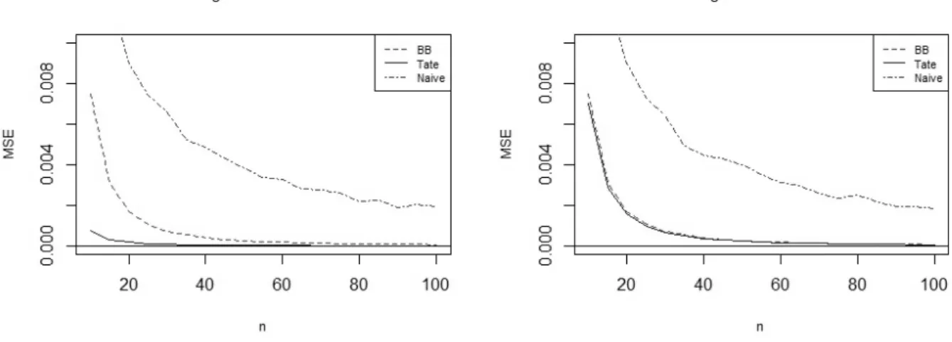
ˆ ξnI = 1− ( 1− 1 n )( τ x(n) )α for 0< τ < x(n), and ˆ ξnII = ( 1− 1 n ) −(1− 2 n ) τα−xα(1) xα (n)−xα(1) for x(1)< τ < x(n). (23) By construction, both estimators are unbiased for ξ(η) =Pη(X > τ) under their correct models. Furthermore, by Example 4, M SE( ˆξn|I Model I) = ( τα θα )2 1 n(n−2),
and by Theorem 1, under Model II,
M SE( ˆξn|I Model II) = Varη( ˆξnI) + (ξ(θ)a+bn)2, wherebnis as given in (19).
Using (9) one can show thatξˆIIn is a biased estimator w.r.t. Model I support for anyfinite sample size, where the bias term is of order1/n. Computing its MSE is complicated and an explicit expression was found only for the case thatα= 1, i.e., truncated uniform random variable.
Fig. 1.The MSE convergence of both estimators and the empirical quantile estimator (based on 1,000 iterations) for the tail probability w.r.t. Model I support, forτ ∈ {0.25,0.75},θ= 1andα= 1.
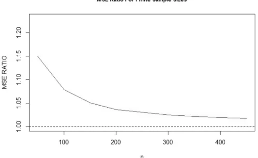
Fig. 2.Asymptotic MSE ratio (Tate/BB) of the estimators of the tail probability w.r.t. Model I support as a function of τforθ= 1andα= 1.
Lemma 1. LetξˆIIn be as in(23)withα= 1. Then the MSE ofξˆIIn w.r.t. ModelIsupport is given by
2τ2n+θ2(n−1)−2τ θn
θ2n2(n−3) . (24)
The proof appears in Appendix A4.
Finally, using Proposition 2, it follows that under Model II M SE( ˆξnII|Model II)≈ 1 n−1 [ (1−ξ)2 (n−3) + ξ2 (n−2) ] ,
whereξ≡ξ(η)is as given in (21). Figures 1 and 2 illustrate the behavior of the MSE of both estimators in Example 5 forfinite and asymptotic sample sizes.
3. ‘REGULAR’ MODELS WITH A POSSIBLE LEFT TRUNCATION PARAMETER In Section 3.1 wefirst present the Erlang distribution as a special case of the natural exponential family (NEF) and illustrate the effects of the possible truncation on the estimator of the ‘regular’ parameter. We then proceed, in Section 3.2 to discuss asymptotic aspects of this problem for general NEF. Finally, in Section 3.3 we illustrate the results with examples.
3.1. Case Study: the Erlang Distribution Letγ ∈[0,∞)befixed,λ >0, and letk= 1,2, . . .. Define
Qk(γ, λ) =
∫ ∞
γ
λkxk−1e−λxdx. (25)
Note thatQk is thek-fold incomplete gamma function, and, in particular,Qk(0, λ) = (k−1)!for any λ >0. As such, we have Qk(γ, λ) = (k−1)! k−1 ∑ i=0 (λγ)i i! e −λγ. (26)
We define the truncated version of thek-stage Erlang distribution, denoted here asErlang(k, λ, γ), by the p.d.f.
f(x;γ, λ) = λ
kxk−1
Qk(γ, λ)
e−λxI[γ < x <∞]. (27) Note the similarity to the definition in Section 2 that appears in (2). By (27), thejth moment of the
Erlang(k, λ, γ)distribution is E(Xj|k, γ, λ) = 1 λj Qk+j(γ, λ) Qk(γ, λ) , j= 0,1,2, . . . . (28)
We now consider the problem of estimatingλunder Model I (i.e.,γ= 0) versus Model II (i.e.,γ >0
unknown). To that end, we use (26) and (28) to calculate
µ0(λ)≡E(X|k,0, λ) and µγ(λ)≡E(X|k, γ, λ) and to obtain that
µ0(λ) = k λ and µγ(λ) = k λ [ 1 +(λγ) ke−λγ kQk(γ, λ) ] . (29)
It can be easily seen from (29) (see also Section 3.2) that the maximum likelihood equation based on a sample ofnobservations fromErlang(k, λ, γ)should satisfy
µ0(ˆλ) = ¯Xn and µγ(ˆλ) = ¯Xn.
That is, the MLEλˆInofλunder Model I (i.e.,γ = 0) and the MLEλˆIIn andγˆn=X(1)ofλandγ under
Model II should satisfy, respectively,
µ0(ˆλIn) = ¯Xn and µγˆn(ˆλ
II
n ) = ¯Xn. (30)
Hence, under Model II,
ˆ λIn= ¯k Xn = k µˆγn(ˆλIIn) PII −−→ λ 1 +(k Qλγ)ke−λγ k(γ, λ) ̸ =λ ,
and thusλInis inconsistent.
To assess the cross-model behavior ofˆλIIn under Model I, wefirst define the bias when estimating the mean function. DefineB(λ, γ)by
B(λ, γ)≡µγ(λ)−µ0(λ) =
(λγ)ke−λγ kQk(γ, λ)
where the equality follows from (29). By Theorem 2 below, γˆn≡X(1)
PII
−−→ γ under Model II and
ˆ
γn −→PI 0under Model I. Hence for everyλ >0we haveB(λ,γnˆ ) −→PI B(λ,0) = 0under Model I. Since by (30) and (31)
µˆγn(ˆλ
II
n) =µ0(ˆλIIn) +B(ˆλIIn,γnˆ ) = ¯Xn, it follows that under Model I,
µ0(ˆλIIn ) = ¯Xn−B(ˆλIIn ,γˆn) PI
−→ µ0(λ)−B(λ, 0) =µ0(λ). (32)
Sinceµ0(·)has a continuous inverse function we also obtain, by the continuous mapping theorem (van
der Vaart, 2000) thatλˆIIn −→PI λ. In other words, we showed that ˆλIIn is consistent and asymptotically unbiased estimator. To conclude this case study, based on the above results, it is clearly preferable, at least from asymptotic point of view, to use the MLE ofλw.r.t. Model II, i.e.,ˆλIIn , to mitigate the possible existence of a left-truncation parameter. The following lemma, which is a special case of Theorem 3, summarizes the cross-model analysis of the case study presented above.
Lemma 2. LetX∼Erlang(k, λ, γ), whereγ ∈[0,∞)is afixed parameter which designates the left
truncation,λ >0is the parameter of interest andk∈N. LetλˆInandˆλIIn be the MLE estimators of λw.r.t. ModelIand ModelIIsupport respectively. Then, under ModelIsupport
ˆ
λIIn −→PI λ, while under ModelIIsupport
ˆ
λIn−−→PII λ
1 +(k Qλγ)ke−λγ
k(γ,λ)
, whereQkis thek-fold incomplete gamma function(see(26)).
In the next subsection we discuss this observation for the general case of NEF distributions, for which the Erlang distribution is a special case.
3.2. Natural Exponential Families with Possible Left Truncation
Letγ ∈[0,∞)befixed,h: [0,∞)→(0,∞)be an absolutely continuous mapping with respect to the Lebesgue measure on the real line, and denote byL(θ, γ)the Laplace transform ofh(x)dx, i.e.,
L(θ, γ) =
∫ ∞
γ
eθxh(x)dx.
Assume that Θγ ≡int{θ∈ R;L(θ, γ)<∞} ̸=ϕ. Then the NEF generated by h(x)dx is given by probability densities of the form
f(x;θ, γ) =h(x)eθx−k(θ,γ)dx, θ∈Θγ, (33) wherek(θ, γ) = logL(θ, γ).
For any fixed γ ∈[0,∞), it is well known that k(θ, γ) is a strictly convex real analytic function on Θγ and kj(θ, γ)≡∂jkj(θ, γ)/∂θj, j= 1,2, . . ., is the jth cumulant corresponding to f(x;θ, γ). Specifically, µγ(θ) =k1(θ, γ) and σ2γ(θ) =k2(θ, γ) are the corresponding mean and variance. Note
that if0≤γ1< γ2 thenΘγ1 ⊆Θγ2, and in particular,Θ0 ⊆Θγ for allγ >0. However, without loss of generality, we assume thatΘ0= Θγ for allγ >0. Note that in the NEF terminology,Mγ ≡k1(Θγ, γ) is the mean parameter space associated with the corresponding NEF, whereasM0 ≡k1(Θ0, γ)satisfies
M0 ⊂ Mγ.
Unlike the Erlang distribution case, we are interested here only in the asymptotic behavior of the MLE of the natural parameterθunder Model I (withγ = 0) and under Model II (withγ >0), as no explicit
relationship as in (29) generally exists. As in the previous section, the maximum likelihood equation based on a sample ofnobservations from (33) should satisfy, for Model I and Model II, respectively,
µ0(ˆθ) = ¯Xn and µγ(ˆθ) = ¯Xn,
provided thatXn¯ ∈ Mγ(a.s.). That is, the MLEθˆInofθunder Model I and the MLEθˆnIIandˆγn=X(1)
ofθandγunder Model II should satisfy, respectively,
µ0(ˆθIn) = ¯Xn and µˆγn(ˆθ
II
n ) = ¯Xn.
More specifically, under Model II, the MLEθˆnIIofθsatisfiesk1(ˆθIIn ,ˆγn) = ¯Xn, withγnˆ ≡X(1), whereas
under Model I, the MLEθˆnIforθsatisfiesk1(ˆθnI,0) = ¯Xn.
In the following theorem we restate the results of Proposition 2 of Dubinin and Vardeman (2003).
Theorem 2. If ModelIholds(i.e.γ = 0)then, asn→ ∞,
√ n(ˆθnI−θ)−→ ND ( 0, 1 k2(θ,0) ) .
Furthermore, if Model II holds (i.e., γ >0) and h(x) is right-continuous at 0, then
(√n(ˆθnII−θ)′, n(ˆγn−γ))′ are asymptotically independent with marginal distributions N(0, k2(θ, γ)−1) and Exp(α)withα=f(γ;θ, γ) =h(γ)eθγ−k(θ,γ), respectively.
Example 6. Let X1, . . . , Xn ∼Exp(λ, γ), so that λ=−θ, where θ is the natural parameter of the distribution, and whereγis the truncation parameter. It can be shown that
k1(θ, γ) =γ−
1
θ.
It can also be shown thatk2(θ, γ) =k2(θ,0) = θ12. This observation means that in the exponential case, truncation is equivalent to shifting by a factor ofγ. Bar-Lev and Boukai (2009) showed that this is the only case for which this unusual property holds.
Consequently, the maximum likelihood estimating equation for Model I is−1θ = ¯Xn, and for Model II is −1θ +X(1) = ¯Xn, sinceX(1) is the MLE of γ. Hence the MLE for the natural parameter is, under
Model I and Model II, respectively,
ˆ θIn=− ¯1 Xn and θˆIIn = 1 X(1)−X¯n .
Example 7. Let X1, . . . , Xn∼Erlang(2, λ, γ), where λ=−θ, θ is the natural parameter, and γ is the truncation parameter. Similarly to the exponential distribution example, k1(θ,0) =−2θ, hence
ˆ
θIn=−X¯2n. Forγ >0, we obtain thatk1(θ, γ) =−2θ +γ−1−γθγ. Some algebra then yields
ˆ θnII =−4 ( ¯ Xn−2X(1)+ √ 4X(1)( ¯Xn−X(1)) + ¯Xn2 )−1 .
Before we discuss cross-model results, we need the following notation. For everyγ >0, define the inverse functionκ−γ1:Mγ 7→Θγbyκ−γ1(µ) =θfor the uniqueθthat satisfiesk1(θ, γ) =µγ. Note that
thisθis indeed unique sincek1(·, γ)is strictly monotonically increasing. It follows from Proposition 2 of
Dubinin and Vardeman (2003) that
κ−γ11(µ)< κ−γ21(µ) (34) for allγ1< γ2, sincek1(θ, γ) is strictly monotonically increasing inγ. Finally, we note that using this
notation we have
ˆ
θnI =κ−01( ¯Xn) and θˆnII =κ−X1(1)( ¯Xn).
We first show that θˆIn is a biased estimator of θ under Model II, with bias that does not vanish asymptotically. We then show thatθˆnIIis an asymptotically efficient estimator ofθunder Model I.
Theorem 3. Assume that ModelIIholds. Then
ˆ
θIn−−→a.s. κ−01(µγ)< κ−γ1(µγ) =θ . (35) If ModelIholds, andh(x)is right-continuous at0, then
√ n(ˆθIIn −θ)−→ ND ( 0, 1 k2(θ,0) ) . See the proof in Appendix A5.
3.3. Examples
Considerfirst the scenario of the negative exponential distribution (i.e., as a special case of thek -stage Erlang distribution discussed above, but withk= 1). Recall that when the MLE forθwas derived under Model I, while Model II actually holds, we obtained thatµγ =−1θ+γ =µ0+γ. Therefore,
− ¯1 Xn
−θ−−→a.s θ
2γ
1−θγ, (36)
which means that the sequence√n(−X¯1
n −θ)goes to infinity asn→ ∞.
Consider now the case that the MLE forθwas derived under Model II, while Model I actually holds. We start with thefinite-sample behavior of the estimatorθˆnII under Model I. It can be shown (see (32)) that its expected value under Model I is nnθ−2, and therefore its bias is given by n−22. Taking the limit asn→ ∞shows that the estimatorθˆIIn is asymptotically unbiased under Model I. Furthermore, direct calculations show that
M SE(ˆθnII|Model I) = (n(n+ 4)−12)θ
2
(n−2)2(n−3) .
The asymptotic behavior of the MLE for the natural parameterθfollows from Theorem 3. Specifically, we have √ n ( 1 X(1)−X¯n − θ ) D −→ N(0, θ2). (37)
We now discuss the Erlang-2 distribution discussed in Example 7. Consider, for instance, the scenario in which the MLE was derived erroneously under Model I support, while Model II holds. It can be shown that in such a case,
− ¯2 Xn −θ
a.s
−−→ −θ3γ2
2 +θγ(θγ−2). (38)
Hence, the sequence√n(−X¯2
n −θ)goes to infinity asn→ ∞. We now consider the scenario in which the MLE was derived under Model II support, but Model I holds. The asymptotic behavior of the MLE for the natural parameter can be derived from Theorem 3 and is similar to (37). Note that thefinite-sample behavior is analytically complicated and is demonstrated using simulations, see Figure 3.
4. CONCLUSIONS
In this work we analyzed the effect of addition of a left-truncation parameter on estimation in continu-ous distribution functions. We discussed two main settings: general continucontinu-ous right-truncated models with possible left truncation, and exponential families with possible left truncation. We investigated the effects of model misspecification on UMVU estimators for thefirst setting, and on maximum likelihood estimators for the second setting. For both settings, we discussed both finite-sample properties and asymptotic behavior of the estimators.
In both settings we showed that mistakenly assuming Model I, when the true model is Model II, leads to a biased estimation with bias that does not vanish asymptotically. On the other hand, assuming
Fig. 3.The MSE ratio (Model II/Model I) for various sample sizes where the true model is Model I. For each sample sizen, 100,000 timesnrandom values fromErlang(2,1,0)distribution were drawn and both MLEs were calculated. The MSEs were calculated by averaging the MLEs of these 100,000 runs, for each sample size.
Model II, when the true model is Model I, leads to an asymptotically unbiased estimation, which is, at least for the exponential family setting, also asymptotically efficient. Nonetheless, it is important to note that estimators constructed under Model II can be more complicated and that there can be a significant efficiency price for estimating under Model II when Model I is correct. In conclusion, based on the results described above, we recommend using Model II when there is a good reason to suspect that the model involves left truncation. When there is no reason to assume left truncation, we recommend to use Model I.
APPENDIX: PROOFS A1. Proof of Theorem 1
Part (i): The expectation of Tate’s UMVU estimator w.r.t. False Mode II can be written as follows E( ˆξn|I Model II) = ∫ θ γ ( ξ(t) +ξ ′(t)g0(0, t) nh(t) ) fSI(t;η)dt= ∫ θ γ ξ(t)fSI(t;η)dt + ∫ θ γ ξ′(t) ( g0(0, t) nh(t) − g0(γ, t) nh(t) ) fSI(t;η)dt+ ∫ θ γ ξ′(t)g0(γ, t) nh(t) fSI(t;η)dt. Note that FSI(t;η) = (g0(γ,t) g0(γ,θ) )n ≡(Fη(t))n, thus fSI(t;η) = nh(t) g0(γ,θ)(Fη(t))
n−1. Therefore, one can
rewrite the equation above in the following way Eη( ˆξnI) = ∫ θ γ ξ(t)fSI(t;η)dt+ g0(0, γ) g0(γ, θ) ∫ θ γ ξ′(t)g0(γ, θ) nh(t) fSI(t;η)dt+ ∫ θ γ ξ′(t)(Fη(t))n−1dt.
By rearranging the equation, using the identities stated before and integration by parts for the last term, one can show that sinceFSI(γ) = 0,FSI(θ) = 1,
Eη( ˆξIn) =ξ(t)FSI(t) θ γ+ g0(0, γ) g0(γ, θ) ∫ θ γ ξ′(t)(Fη(t))n−1dt=ξ(θ) +bn,
witha= g0(0,γ)
g0(γ,θ)andbn=a ∫θ
γ ξ′(t)(Fη(t))
n−1dt. Again, by integration by parts we obtain that
bn=a ( ξ(θ)− ∫ θ γ ξ(t)(n−1)h(t)(g0(γ, t)) n−2 (g0(γ, θ))n−1dt ) , which completes the proof of thefirst part.
Part (ii): The proof is straightforward, and is given by E( ˆξnII|Model I) = ∫ θ 0 ∫ t 0 ˆ ξnII(y, t)fSII(y, t;η0)dy dt= ∫ θ γ ∫ t γ ˆ ξIIn (y, t)fSII(y, t;η0)dy dt + ∫ γ 0 ∫ t 0 ˆ ξIIn (y, t)fSII(y, t;η0)dy dt+ ∫ θ γ ∫ γ 0 ˆ ξnII(y, t)fSII(y, t;η0)dy dt =ξ(η) +d1n+d2n.
A2. Proof of Proposition 1
The expectation of the squared Tate’s UMVU estimator w.r.t. Model I support can be explicitly written as E(( ˆξnI)2|Model I) =Eη0 ( ξ2(t) +2ξ(t)ξ ′(t)g 0(0, t) nh(t) + ( ξ′(t)g0(0, t) nh(t) )2) . Note that since gnh(0(,tt))fSI(t;η0) =FSI(t;η0), one can show that
Eη0 ( ( ˆξnI)2)= ∫ θ 0 ξ2(t)fSI(t;η0)dt+ ∫ θ 0 2ξ(t)ξ′(t)FSI(t;η0)dt+ ∫ θ 0 ( ξ′(t)g0(0, t) nh(t) )2 fSI(t;η0)dt .
By using integration by parts and the facts thatFSI(0) = 0andFSI(θ) = 1, one can show that
Eη0 ( ( ˆξIn)2)=ξ2(t)FSI(t) θ 0+ ∫ θ 0 ( ξ′(t)g0(0, t) nh(t) )2 fSI(t;η0)dt =ξ2(θ) + ∫ θ 0 ( ξ′(t)g0(0, t) nh(t) )2 fSI(t;η0)dt .
A3. Proof of Proposition 2 LetξˆII
n be the Model II UMVUE ofξ(γ, θ)as is given in (15). Then using the law of total variance we can express the variance ofξˆnIIin the following way
Varη( ˆξIIn ) =Eη ( Varη( ˆξnII|X(1)) ) + Varη ( Eη( ˆξnII|X(1)) ) . Starting with thefirst term, by using (17), we know that
ˆ
ξnII(y, t) =r(y, t) +r2(y, t)g0(y, t) (n−1)h(t) ,
wherer2 =∂r/∂θ. Therefore, by using Proposition 1 we can immediately calculateVarη( ˆξnII|X(1)=y),
which is simply an integration of the squared second term in the expression above w.r.t. the density function ofX(n)over Model II support, i.e.,
Varη( ˆξnII|X(1)=y) = ∫ θ y ( r2(y, t)g0(y, t) (n−1)h(t) )2 fX(n)(t;η)dt .
In order to computeEη
(
Varη( ˆξnII|X(1)) )
we have to integrateVarη( ˆξnII|X(1) =y)over all possible values
ofX(1)w.r.t. Model II support. More specifically,
∫ θ γ [ ∫ θ y ( r2(y, t)g0(y, t) (n−1)h(t) )2 fX(n)(t;η)dt ] fX(1)(y;η)dy, which completes thefirst term ofVarη( ˆξnII).
Proceeding to the second term, using (16) we know that Eη( ˆξnII|X(1) =y) =ξ(y, θ)−
ξ1(y, θ)g0(y, θ)
nh(y) .
Utilizing Proposition 1 to calculate the variance of the expression presented above, one should integrate the squared second term of this expression w.r.t. the density functionX(1)over Model II support, i.e.,
Varη ( Eη( ˆξIIn |X(1)) ) = ∫ θ γ ( ξ1(y, θ)g0(y, θ) nh(y) )2 fX(1)(y;η)dy,
which completes the computation of the second term ofVarη( ˆξIIn )and concludes the proof.
A4. Proof of Lemma 1
Letξ(η)be as in (22) but withα= 1, i.e.,ξ(η) = θ−θτ. We would like to compute
M SE( ˆξnII|Model I) =Eη0 ( ˆ ξnII−θ−τ θ )2 =Eη0 (ˆ ξnII)2−2(θ−τ) θ Eη0ξˆ II n + ( θ−τ θ )2 . (39) Sinceα= 1, we haveh(x) = 1andg0(0, θ) =θ. Hence, from (9), we have
fSII(y, t;η0) = n(n−1)(t−y)n−2 θn , for 0≤y < t≤θ . We also have ˆ ξIIn (y, t) = ( 1− 1 n ) −(1− 2 n )τ −y t−y for y < τ < t . Hence Eη0ξˆ II n = ∫ θ 0 ∫ t 0 ˆ ξIIn (y, t)fSII(y, t;η0)dy dt = ∫ θ 0 ∫ t 0 (( 1− 1 n ) −(1− 2 n )τ −y t−y ) n(n−1)(t−y)n−2 θn dy dt = ∫ θ 0 ∫ t 0 ( C1(t−y)n−2+C2(t−y)n−3+C3y(t−y)n−3 ) dy dt = ∫ θ 0 ( C1D(n−2,0) +C2D(n−3,0) +C3D(n−3,1)|ty=0 ) dt , where C1 ≡ ( 1− 1 n )n(n−1) θn = (n−1)2 θn , C2 ≡ − ( 1− 2 n )τ n(n−1) θn =−τ (n−1)(n−2) θn , C3 ≡ ( 1− 2 n )n(n−1) θn =− C2 τ ,
andD(n, k, c)≡xk(x−c)nand where D(n,0)≡ ∫ (t−y)ndy=− 1 (n+ 1)(y−t) n+1, D(n,1)≡ ∫ (t−y)ny dy=−(t−y) n+1(t+ (n+ 1)y) (n+ 1)(n+ 2) , D(n,2)≡ ∫ (t−y)ny2dy=−(t−y) n+1(8t2+ 8t(n+ 1)y+ 4(n+ 1)(n+ 2)y2) 4(n+ 1)(n+ 2)(n+ 3) . Hence Eη0ξˆ II n (y, t) = C1 n−1 ∫ θ 0 tn−1dt+ C2 n−2 ∫ θ 0 tn−2dt+ C3 (n−1)(n−2) ∫ θ 0 tn−1dt = ( C1 n−1 + C3 (n−1)(n−2) ) θn n + C2 n−2 θn−1 n−1 = 1− τ θ. We now computeEη0 ( ( ˆξnII)2): Eη0 ( ( ˆξnII)2)= ∫ θ 0 ∫ t 0 (ˆ ξIIn (y, t))2fSII(y, t;η0)dy dt = ∫ θ 0 ∫ t 0 (( 1− 1 n ) −(1− 2 n )τ −y t−y )2n(n−1)(t−y)n−2 θn dy dt = ∫ θ 0 ( E1D(n−2,0) +E2D(n−4,0) +E3D(n−4,2))ty=0dt + ∫ θ 0 ( E1,2D(n−3,0) +E1,3D(n−3,1) +E1,2D(n−4,1)) t y=0dt, where E1 ≡ ( 1− 1 n )2n(n−1) θn = (n−1)3 θnn , E2 ≡ ( 1− 2 n )2τ2n(n−1) θn =− τ2(n−1) (n−2)2 θnn , E3 ≡ ( 1− 2 n )2n(n−1) θn = (n−1) (n−2)2 θnn , E1,2 ≡ −2τ ( 1− 1 n )( 1− 2 n )n(n−1) θn =− 2τ(n−1)2(n−2) θnn , E1,3 ≡2τ ( 1− 1 n )( 1− 2 n )n(n−1) θn = 2 (n−1)2(n−2) θnn , E2,3 ≡ −2τ ( 1− 2 n )2n(n−1) θn =− 2τ(n−2)2(n−1) θnn . Hence Eη0 ( ( ˆξnII)2)=− ∫ θ 0 ( E1 (t−y)n−1 n−1 +E2 (t−y)n−3 n−3 ) t y=0 dt − ∫ θ 0 ( E3 (t−y)n−3(8t2+ 8(n−3)ty+ 4(n−3)(n−2)y2) 4(n−3)(n−2)(n−1) +E1,2 (t−y)n−2 n−2 ) t y=0 dt − ∫ θ 0 ( E1,3 (t−y)n−2(t+ (n−2)y) (n−2)(n−1) +E2,3 (t−y)n−3(t+ (n−3)y) (n−3)(n−2) ) t y=0 dt
= ∫ θ 0 ( E1tn−1 n−1 + E2tn−3 n−3 + 8E3tn−1 4(n−3)(n−2)(n−1) ) dt + ∫ θ 0 ( E1,2tn−2 n−2 + E1,3tn−1 (n−2)(n−1)+ E2,3tn−2 (n−3)(n−2) ) dt = ( E1 n−1 + 2E3 (n−3)(n−2)(n−1)+ E1,3 (n−2)(n−1) ) θn n + ( E1,2 n−2+ E2,3 (n−3)(n−2) ) θn−1 n−1 + E2θn−2 (n−3)(n−2) = n 3−3n2+n−1 n2(n−3) − 2τ(n2−3n+ 1) θ n(n−3) + τ2(n−1) (n−2) θ2n(n−3) .
Substituting the expressions we obtained forEη0ξˆ
II
n andEη0 (
( ˆξnII)2)in (39), and some simplifying we obtain the result given in (24).
A5. Proof of Theorem 3
Thefirst assertion follows from the continuous mapping theorem, see van der Vaart (2000). Indeed,
ˆ
θnI =κ−01( ¯Xn) a.s.
−−→κ−01(µγ). The inequality in (35) follows from (34).
We now move to the second assertion. Note that when Model I holds √
n(ˆθIIn −θ) =√n(ˆθIIn −θˆnI) +√n(ˆθIn−θ). Since by Theorem 2,√n(ˆθIn−θ)−→ ND (0,k 1
2(θ,0) )
, it is enough to show that√n(ˆθIIn −θˆIn)−→D 0. We define the functiong: M0×R7→Θ0 byg(µ, γ) =θfor the uniqueθ that solvesk1(θ, γ) =µ.
It follows from Proposition 2 of Dubinin and Vardeman (2003) that thisθis unique and thatg(µ, γ)is continuously differentiable. Note thatθˆI
n=g( ¯Xn,0)andθˆnII =g( ¯Xn, X(1)). Write √ n(ˆθnII−θˆnI) =√n(g( ¯Xn, X(1))−g( ¯Xn,0) ) =√n ∂ ∂γg( ¯Xn, r)X(1)
for some0< r < X(1). Note thatX(1) =op(n−1/2)and that ∂γ∂ g( ¯Xn, r) =Op(1)because the function is bounded in the vicinity of0. Hence we obtain that
√
n(ˆθnII−θˆnI) =n1/2Op(1)op(n−1/2)−→PI 0, which concludes the proof.
ACKNOWLEDGMENTS
The authors are grateful to anonymous reviewer for helpful suggestions and comments. Thefirst and the second authors were funded in part by Israel Science Foundation grant 1308/12.
REFERENCES
1. S. K. Bar-Lev and B. Boukai, “Minimum Variance Unbiased Estimation for Families of Distributions Involving Two Truncation Parameters”, J. Statist. Plann. Inf.12, 379–384 (1985).
2. S. K. Bar-Lev and B. Boukai,“A Characterization of the Exponential Distribution by Means of Coincidence of Location and Truncated Densities”, Statist. Papers50(2), 403–405 (2009).
3. P. J. Bickel, “Parametric Robustness: Small Biases can be Worthwhile”, Ann. Statist. 12 (3), 864–879 (1984).
4. K. P. Burnham and D. R. Anderson, Model Selection and Multimodel Inference : A Practical Information-Theoretic Approach(Springer, 2002).
6. T. M. Dubinin and S. B. Vardeman,“Likelihood-Based Inference in Some Continuous Exponential Families with Unknown Threshold Parameters”, J. Amer. Statist. Assoc.98(463), (2003).
7. R. C. Elandt-Johnson,Survival Models and Data Analysis(Wiley, 1999). 8. J. F. Lawless,Statistical Models and Methods for Lifetime Data(Wiley, 2003).
9. R. F. Tate,“Unbiased Estimation: Functions of Location and Scale Parameters”, Ann. Math. Statist.30(2), 341–366 (1959).
10. A. W. van der Vaart,Asymptotic Statistics(Cambridge Univ. Press, 2000).