Distributed Methods for Composite Optimization: Communication Efficiency, Load-Balancing and Local Solvers

(1)

Lehigh University

Lehigh Preserve

Theses and Dissertations

9-1-2018

Distributed Methods for Composite Optimization:

Communication Efficiency, Load-Balancing and

Local Solvers

Chenxin Ma

Lehigh University, [email protected]

Follow this and additional works at:

https://preserve.lehigh.edu/etd

Part of the

Systems Engineering Commons

This Dissertation is brought to you for free and open access by Lehigh Preserve. It has been accepted for inclusion in Theses and Dissertations by an

authorized administrator of Lehigh Preserve. For more information, please [email protected].

Recommended Citation

Ma, Chenxin, "Distributed Methods for Composite Optimization: Communication Efficiency, Load-Balancing and Local Solvers" (2018).Theses and Dissertations. 4310.

(2)

Distributed Methods for Composite Optimization:

Communication Efficiency, Load-Balancing and Local Solvers

by

Chenxin Ma

Presented to the Graduate and Research Committee of Lehigh University

in Candidacy for the Degree of Doctor of Philosophy

in

Industrial and Systems Engineering

Lehigh University August 2018

(3)

c

Copyright by Chenxin Ma 2018

(4)

Approved and recommended for acceptance as a dissertation in partial fulfillment of the requirements for the degree of Doctor of Philosophy.

Date

Dissertation Advisor

Committee Members:

Dr. Martin Tak´aˇc, Committee Chair

Dr. Katya Scheinberg

Dr. Frank E. Curtis

(5)

Acknowledgments

I would like to first of all thank to my advisor Martin Tak´aˇc. He is the first person

that I worked so closely with in my life. He has shown me how to work as a researcher with passion, how to be creative by critical thinking. He can always ask insightful and fundamental questions that force me to think more deeply about the problem and inspire me to find the solution. He has also spent a tremendous amount of time in improving my presentation skills. He has taught me, either directly or indirectly, many more things than I could have expected from an advisor. What I have learned from him is not only concentrated in this thesis, but also very helpful in my life.

Also, I would like to thank Katya Scheinberg and Frank E. Curtis for sharing their knowledge and understanding on optimization. They can always get straight to the heart of a complicated problem by only a few words. Both of them gave me priceless support and advice on my research and career development during the past few years. To me, OptML is a group for us to discuss ideas and papers, as well as a family where I can always find funny and unique experiences. I am also very grateful to Rachael Tappenden for her constructive suggestions and research collaborations. Her suggestion and help across the sea is so important to me in the completion of this thesis. It is my pleasure to have these researchers in my committee.

Perhaps nothing would happen without my undergraduate study at Nankai University. I want to thank Bowei Zhang, Qun bao, Cheng Liu from School of Economics, Zhi Song from School of Physics and Wei Geng, Yunhua Xue from School of Mathematics. From these scholars, I am able to see the beauty of different majors and view a problem from different angles. They would like to discuss everything with me, encouraged me to find my

(6)

real interest and told me how important it is. To me, their suggestion and encouragement completely changed my life. I can not imagine what a person I would become without talking to them.

I am also grateful to many researchers I had chance to collaborate with, especially to

Martin Jaggi, Peter Richt´arik, Jakub Koneˇcn´y, Virginia Smith and Jakub Mareˇcek. The

interesting conversations we have had greatly improve my understanding of various topics and inspire me a lot. Also, I would like to take this opportunity to especially thank Yan Xu, Jun Liu, Fei Tong and Young Ju Lee, whom I was lucky enough to work with during my internship and master’s study. I appreciate their time on showing me different interesting real-world problems and guiding me through these years.

I feel very lucky to knowing my friends and graduate students at Lehigh, Xi He, Wei Xia, Yuhai Hu, Mohammadreza Samadi, Majid Jahani, Rui Shi, Yinan Liu, Xiaocheng Tang and Mark Bai, to name a few. I quite enjoy the time spent with them of chatting about research, life and future. They make my life at Lehigh lots of fun.

Further, I want to say I forever love my father Xianfa Ma, my mother Ruimin Xu, my wife Wenqing Ma and my son Miles Ma who is expected to be born later this month. Hope we will have a safe delivery and a healthy baby. My parents have helped me grow a lot of good habits since I was a child, for example, keeping writing a diary. I have found many great benefits from keeping writing something everyday. One of them is, I was able to write the gratitude to my wife into the diary, otherwise it could be too long to be here. Finally, I have a special note to thank Doctor Thomas Novak from Lehigh health center and the doctor from St. Luke Hospital for keeping me healthy.

(7)

List of Tables

1.1 Examples of commonly used loss functions. . . 9

2.1 Datasets used for numerical experiments. . . 37

2.2 Local solvers used in numerical experiments. . . 38

2.3 Optimal H for different local solvers for rcv1 test dataset. . . 39

4.1 Loss functions satisfying Assumption 4.1 and the parameter M. . . 67

4.2 Communication efficiency of several distributed algorithms when the regu-larization parameterλ∼1/√n. . . 68

4.3 Comparison of computation between different algorithms. . . 73

4.4 Comparison of communication between different algorithms. . . 73

4.5 Communication cost (second) of two algorithms on news20 dataset . . . 74

4.6 Communication cost (second) of two algorithms on a1a dataset . . . 74

(11)

List of Figures

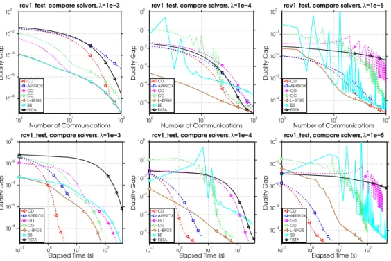
2.1 Performance of different local solvers. . . 38

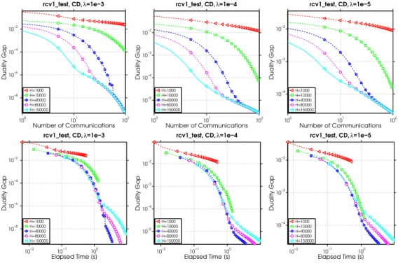
2.2 Varying the number of iterations of CD as a local solver. . . 39

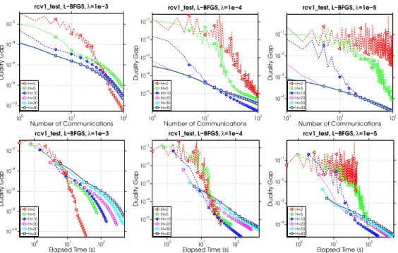
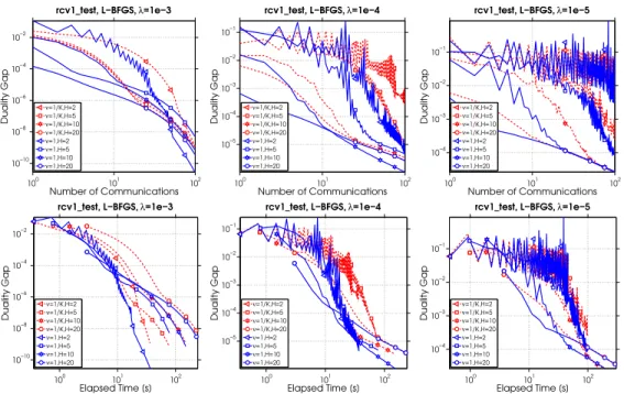
2.3 Varying the number of iterations of L-BFGS as a local solver. . . 40

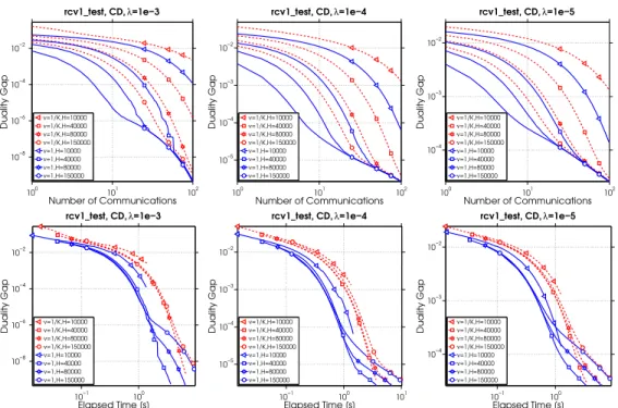
2.4 Adding vs Averaging for CD as the local solver. . . 41

2.5 Adding vs Averaging for L-BFGS as the local solver. . . 42

2.6 Adding vs Averaging for CG as the local solver. . . 42

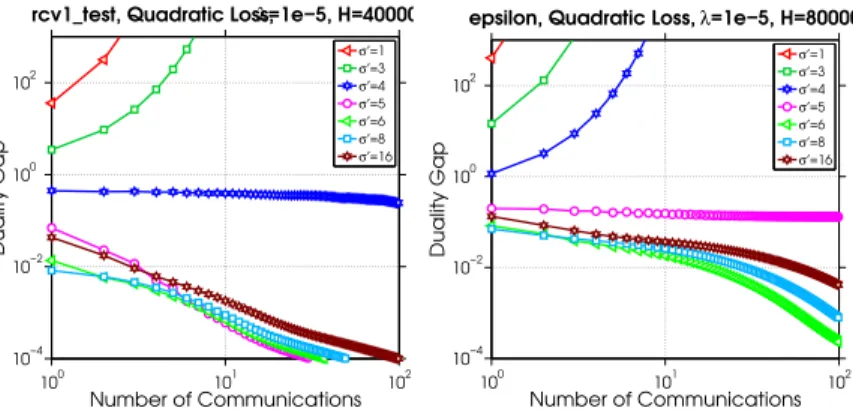
2.7 The effect of σ0 on convergence for the rcvtest and epsilon datasets dis-tributed across 8 machines. . . 43

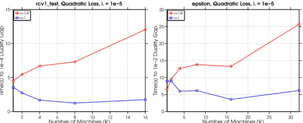
2.8 The effect of increasing the number of machinesK on the time (s) to reach a solution with expected duality gap. . . 44

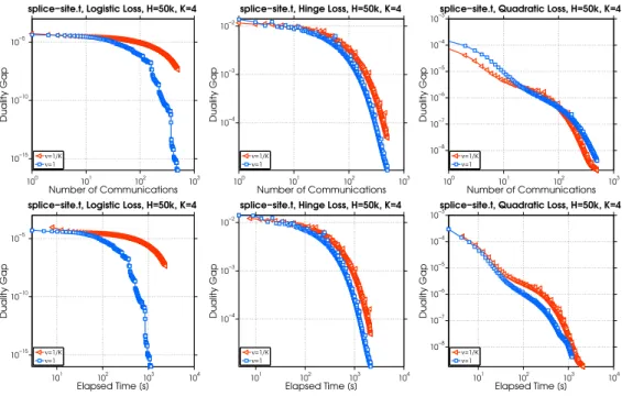
2.9 Performance of Algorithm 2 on splice-site.t dataset. . . 45

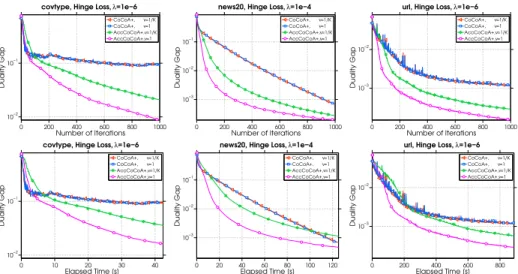
3.1 Duality gap as a function of iterations (top row) and elapsed time (bottom row) when solving hinge-loss SVM problems. . . 64

3.2 Duality gap as a function of iterations (top row) and elapsed time (bottom row) when solving hinge-loss SVM problems with different regularization values (λ) on the urldataset. . . 64

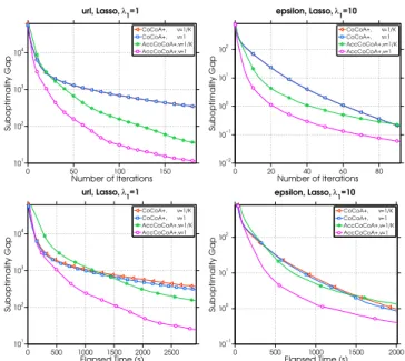
3.3 Sub-optimality gap as a function of iterations (top row) and elapsed time (bottom row) when solving Lasso problems. . . 65

3.4 Number of iterations and running time required to reach a tolerance of 10−3_{on the} duality gap as the inner iteration limit (H) is varied. . . 65

(12)

4.2 Norm of gradient vs. the round of communication, as well as norm of

gra-dient vs. elapsed time. . . 75

4.3 Comparison of different number of samples used in Preconditioning by

run-ning DiSCO-F. . . 77

4.4 Comparison of different number of samples used in approximating Hessian

by running DiSCO-F. . . 78

5.1 Left: Randomly generated two classes of 2D data. Right: A 2D illustration

for Option 1. The blue, red and green points represent {wt},{vt},{w++t }

respectively. . . 95

5.2 Evolution of the gapf(wt)−φ?t for each algorithm compared with the

num-ber of function evaluations and cputime. . . 108

5.3 Empirical convergece rates for ASUESA and for OQA with different numbers

of bisection steps (b= 2,5,20). The black dots are 1−q_Lµ. . . 108

5.4 Empirical convergece rates for SUESA and ASUESA and 1− µ_L(green line)

and 1−q_Lµ (black line). . . 110

5.5 Comparison of how gaps between the objective values and the minimum

amount of the lower bounds decreases for different algorithms. . . 111

5.6 Empirical convergece rates for CUESA and ACUESA and 1−µ_L(green line)

(13)

Abstract

The scale of modern datasets necessitates the development of efficient distributed opti-mization methods for composite problems, which have numerous applications in the field of machine learning. A critical challenge in realizing this promise of scalability is to develop efficient methods for communicating and coordinating information between distributed ma-chines, taking into account the specific needs of machine learning algorithms. Recent work in this area has been limited by focusing heavily on developing highly specific methods for the distributed environment. These special-purpose methods are often unable to fully leverage the competitive performance of their well-tuned and customized single machine counterparts. Further, they are unable to easily integrate improvements that continue to be made to single machine methods. To this end, we present a framework for distributed optimization in Chapter 2 and its accelerated version in Chapter 3 that allow the flexibil-ity of arbitrary solvers to be used on each machine locally, and yet maintains competitive performance against other distributed methods. We give strong primal-dual convergence rate guarantees for our framework that hold for arbitrary local solvers. We demonstrate the impact of local solver selection both theoretically and in an extensive experimental comparison. Further, in Chapter 4 we proposed algorithmic modifications to an existed distributed inexact dumped Newton method, which lead to less round of communications and better load-balancing.

In Chapter 5, we introduce the concept of an Underestimate Sequence (UES), which is a natural extension of Nesterov’s estimate sequence. Our definition of a UES utilizes three sequences, one of which is a lower bound of the objective function. The question of how to construct an appropriate sequence of lower bounds is also addressed, and we present lower

(14)

bounds for strongly convex smooth functions and for strongly convex composite functions, which adhere to the UES framework. Further, we propose several first order methods for minimizing strongly convex functions in both the smooth and composite cases. The algo-rithms, based on efficiently updating lower bounds on the objective functions, have natural stopping conditions, which provides the user with a certificate of optimality. Convergence of all algorithms is guaranteed through the UES framework, and we show that all presented algorithms converge linearly, with the accelerated variants enjoying the optimal linear rate of convergence.

(15)

Chapter 1 Introduction

As the information and computing technology develops, it is now commonplace to attack problems from many fields through data analysis, particularly through the use of statis-tical and machine learning algorithms on what are often large datasets. This trend has been referred to as Big Data, and it has had a significant impact in areas as varied as artificial intelligence, Internet applications, computational biology, finance, marketing and logistics [10].

Though these problems arise in diverse application domains, they all share some key characteristics. First, the datasets are often extremely large. They may consist of millions or even billions of training samples; They may become very high-dimensional, because it is now possible to measure and store very detailed information of each sample. Thus, the datasets are often stored or even collected in a distributed manner. Second, many such problems can be formulated in the framework of composite optimization. As a result, it has become of central importance to develop distributed optimization algorithms for convex composite problems, to capture the complexity of modern data and scale well under modern parallel computing architecture.

In general, there are following two main challenges on developing distributed optimiza-tion algorithms.

• On typical high performance computing clusters, communication between machines is

(16)

when trying to translate the highly tuned existing single machine algorithms to the distributed setting, great care must be taken to avoid too much communications through network. Thus, for distributed optimization, the round of communications between nodes should be minimized. At least, we should be able to balance the time that is spent on computation and communication.

• Load-balancing between machines greatly affects the efficiency of distributed

algo-rithms. Amdahl’s law [61] implies that if a parallel algorithm spend more time only on one of the nodes (usually the master node), then the possible speed-up from uti-lizing more machines will becomes much lower. Hence, a distributed algorithm that scales well should try to distribute computation tasks evenly to each machine. In the first part of this dissertation, we present techniques to address the above two dif-ficulties. In the later part, we focus on proposing new first order methods, which can be used as the local solvers of our distributed framework. Overall, we are interested in developing distributed methods that reduce the communication cost, and developing non-linear optimization algorithms on single machines to further improve the efficiency of local computation.

The dissertation is organized as follows. In rest of Chapter 1, we introduce relevant background of distributed optimization and mathematical settings on which the later chap-ters are based. In Chapter 2 we develop and analyze the proposed distributed framework

CoCoA+ under different assumptions on the problem. In Chapter 3, based on Nesterov’s

accelerating scheme, we presents an variant of CoCoA+ which improves the convergence

rate. Chapter 4 includes a series of algorithmic modifications on an existed distributed algorithm to reduce the number of communications and improve the scalability. Finally, we extend the idea of Estimate Sequences and propose new first order methods which reach the optimal convergence rate in Chapter 5.

(17)

1.1 Background and Settings

We start by introducing some definitions and notations, followed by the problem setting and necessary assumptions.

1.1.1 Definitions

The following standard definitions will be used throughout the thesis. For simplicity, we usek · k to denote k · k2.

Definition 1.1(L-Lipschitz Continuity). A functionh:Rm →RisL-Lipschitz continuous

if∀u,v∈_Rm_{, we have}

|h(u)−h(v)| ≤Lku−vk. (1.1)

Definition 1.2 (L-Bounded Support). A function h : Rm → R∪ {+∞} has L-bounded

support if its effective domain is bounded byL, i.e.,

h(u)<+∞ ⇒ kuk ≤L . (1.2)

Definition 1.3 (β-Smoothness). A functionh:Rm →Risβ-smooth if it is differentiable

and its gradient isβ-Lipschitz continuous, or equivalently,

h(u)≤h(v) +h∇h(v),u−vi+ β

2ku−vk

2 _∀_u_,_w_∈

Rm. (1.3)

Definition 1.4 (β-Strong Convexity). A differentiable functionh :Rm→R isβ-strongly

convex forβ ≥0 if,

h(u)≥h(v) +h∇h(v),u−vi+β

2ku−vk

2 _∀_u_,_v_∈

Rm. (1.4)

Definition 1.5 (Convex Conjugate). The convex conjugate of a function h :Rm → R is

the functionh∗:Rm →Rdefined by,

h∗(v) = sup

u∈_Rm

(18)

We also define the notation [n] :={1,2, ..., n} for any integern >0. All the notations throughout the dissertation are summarized in the appendix.

1.1.2 A Description of Problems

We are interested in solving the following pair of composite optimization problems:

min α∈_Rn h O_A(α) := f(Xα) + g(α) i, (A) min w∈_Rd h O_B(w) := f∗(w) + g∗(−X>w) i. (B) Here α ∈_Rn _and _w_∈

Rd are variable vectors,X := [x1;. . .;xn]∈Rd×n is a data matrix

with column vectors xi ∈ Rd, i ∈ [n]. We will assume without loss of generality that

∀i:kxik ≤ 1. y∈ Rn is a vector containing the label for each data vector. Functions f∗

and g∗ are conjugates of convex functionsf :Rd→R and g:Rn→R, respectively.

The relationship of problems (A) and (B) is known as Fenchel-Rockafellar duality [8], as stated in Proposition 1.6. Note that while dual problems are typically presented as a pair of (min, max) problems, we have equivalently reformulated both (A) and (B) to be minimization problems for consistence.

Proposition 1.6. (Appendix C in [24]) Problem (B) is the dual problem of (A).

It is well known [57, 70, 66, 24] that the first-order optimality conditions give rise to a natural mapping that relates pairs of primal and dual variables. The mapping employs the

linear map given by the dataX, and maps any dual variableα∈Rnto a primal candidate

vectorw∈_Rd _{as follows:}

w=w(α) :=∇f(Xα). (1.6)

For this mapping, under the assumptions that we make in Section 1.1.3 below, it holds

that if α? is an optimal solution of (A), then w(α?) is an optimal solution of (B). In

(19)

duality gap function as

G(α) :=O_A(α)− − O_B(w(α)), (1.7)

then G(α?_{) = 0, which ensures that by solving the dual problem (A) we also solve the}

original primal problem of interest (B). Moreover, the duality gap at any point provides a practically computable upper bound on the unknown primal as well as dual optimization error (sub-optimality), since

OA(α)≥ OA(α?) =−OB(w?)≥ −OB(w(α)).

As we will later see, there are many benefits to leveraging this primal-dual relationship, including the ability to use the duality gap as a certificate of solution quality, and, in the distributed setting, as a tool through which we can effectively distribute computation.

1.1.3 Assumptions

We make the following assumption on problem (A).

Assumption 1.7. f is(1/τ)-smooth, and the functiongis separable and defined as a sum

of n convex functions, i.e., g(α) = Pn

i=1gi(αi), with each gi : R → R having L-bounded

support.

Proposition 1.8(Theorem 6 in [31]). A convex functionh:Rm→Risβ-strongly convex

if and only if its convex conjugate h∗ is _β1 smooth.

Proposition 1.9. A closed convex function h:R→R has L-bounded support if and only

if its convex conjugateh∗ isL-Lipschitz continuous.

Proof. Let us first assume function h has L-bounded support. ∀v1 ∈ _R, let ˆu denote the

optimal solution of sup_u(v1u−h(u)) and we know |uˆ| ≤ L. Thus, h∗(v1) = sup_u(v1u−

h(u)) =v1uˆ−h(ˆu). Then, ∀v2∈R, we have,

h∗(v1)−h∗(v2)≤v1uˆ−h(ˆu)−sup

u

(20)

≤v1uˆ−h(ˆu)−v2uˆ+h(ˆu)

≤(v1−v2)ˆu≤L|v1−v2|.

Thus,h∗isL-Lipschitz continuous. It is left to prove thathisL-bounded support assuming

h∗ is L-Lipschitz continuous. Since h is closed convex, we have h = h∗∗. Thus, for some

u > L, h(u) = sup v (uv−h∗(v)) ≥ −h∗(0) + sup v (uv−(h∗(v)−h∗(0))) ≥ −h∗(0) + sup v (uv−L|v−0|) ≥ −h∗(0) + sup v>0 (uv−Lv) =∞.

A similar argument holds for u < −L. Thus, for any u such that |u| > L we have that

h(u) =∞, which proves that hhas L-bounded support.

Given the duality between the problems (A) and (B) and above propositions,

Assump-tion 1.1.3 can be equivalently stated as assuming that in problem (B), f∗ is τ-strongly

convex, and the function g∗(−X>w) = Pn

i=1gi∗(−x>i w) is separable with each g∗i being

L-Lipschitz.

1.1.4 Applications

Problems (A) and (B) appear frequently in the application of machine learning. Here we introduce some examples, and how to map them to at least one of problems (A) and (B).

1. Lasso [73]. We can map the L1-regularized least squares regression problem:

min α∈_Rn 1 2kXα−yk 2₊_λ_k_α_k 1, (1.8)

to objective (A) by letting f(Xα) = 1₂kXα−yk2 _and _g₍_α_{) =}P

igi(αi) =Piλ|αi|,

where λ > 0 is the regularization parameter. In this mapping, n represents the

(21)

Loss function `i(a) `∗i(b)

Quadratic loss 1₂(a−yi)2 1₂b2+yib

Hinge loss max{0, yi−a} yib, b∈[−1,0]

Squared hinge loss (max{0, yi−a})2 b

2

4, b∈[−∞,0]

Logistic loss log(1 + exp (−yia)) −_yb

ilog −b yi +1 + _yb i log1 + _yb i ,_yb i ∈(−1,0)

Table 1.1: Examples of commonly used loss functions.

the lasso objective to (B) directly, asf∗ must beτ-strongly convex whileL1-norm is

not.

2. L2-Regularized Empirical Risk Minimization [74]. We can represent aL2-regularized

empirical risk minimization (ERM) by mapping the problem:

min w∈_Rd 1 n n X i=1 `i(x>i w) + λ 2kwk 2_, _(1.9) to objective (B) by letting g∗(−X>w) = Pn i=1gi∗(−x>i w) = Pn i=1n1`i(x > i w) and f∗(w) = λ₂kwk2_{, where} _`

i(·) is some convex loss function for i ∈ [n] and λ > 0.

In this mapping, drepresents the number of features, and n the number of training

points. The dual problem of (1.9) can be mapped to (A) as:

min α∈Rn 1 n n X i=1 `∗_i(−αi) + λ 2k 1 λnXαk 2_, _(1.10) whereg(α) =Pn i=1gi(αi) =Pni=1n1` ∗

i(−αi) andf(α) = λ₂k_λn1 Xαk. Here`∗i(·) is the

convex conjugate of `i(·). Table 1.1 lists several examples of `i and `∗i. If applying

hinge loss, then (1.9) will become Support Vector Machine (SVM) problem:

min w∈_Rd 1 n n X i=1 max0, yi−x>i w + λ 2kwk 2_. _(1.11)

3. Elastic Net Regression [84]. We can map elastic-net regularized least squares

regres-sion problem: min u∈Rp 1 2kXu−yk 2₊_η_k_u_k 1+ λ 2kuk 2_, _(1.12)

(22)

to either objective (B) or (A). To map to objective (B), let f(Xα) = 1₂kXα−yk2

andg(α) =P

igi(αi) =Piη|αi|+λ₂α2i, whereη >0 andλ >0 are two regularization

parameters. In this case,nis the number of features anddis the number of training

points. To map to (A), let g(−X>w) = P

igi∗(−x>i w) =

P

i12(x >

i w−yi)2 and

f∗(w) =ηkwk₁+λ₂kwk2_{, setting}_d_{to be the number of features and} _n _{the number}

of training points.

1.1.5 Data Partition

To view our setup in the distributed environment, We assume that dataset {xi, yi}ni=1 is

residing on K machines in a distributed way, with every machine only holding a part of

the whole dataset. In the same way we split the dual variablesα, with each corresponding

to an individual data point xi. The given data distribution is described using a partition

P1, . . . ,PKthat corresponds to the indices of data and dual variables residing on machinek.

Formally, Pk ⊆ {1,2, . . . , n} for each k∈ [K] :={1, ..., K},Pk∩ Pl = ∅ whenever k6= l,

and SK

k=1Pk ={1,2, . . . , n}.

In order to efficiently use this structure in the text, we introduce the following notation.

For anyh∈_Rn_{we use the notation}_h[k]_∈

Rn for the vector

h[_ik]:=        0, ifi /∈ P_k, hi, otherwise. (1.13)

Note that, in particular we haveh=PK

k=1h[k].Analogously, we writeX[k] for the matrix

(23)

Chapter 2 A Framework for Communication

Efficient Distributed Optimization

In this chapter, we propose a general communication efficient distributed framework that can employ arbitrary single machine local solvers in this chapter. In Section 2.2, we present

our framework, CoCoA+, which can cover general non-strongly convex regularizers,

in-cluding L1-regularized problems like lasso, sparse logistic regression, and elastic net reg-ularization, and show how earlier work can be derived as a special case. In Section 2.3, we provide convergence guarantees for the class of convex regularized loss minimization objectives, leveraging a novel approach in handling non-strongly convex regularizers and non-smooth loss functions. The resulting framework has markedly improved performance over state-of-the-art methods, as we illustrate with an extensive set of experiments on real distributed datasets in Section 2.5.

2.1 Motivation and Assumptions

There are two motivations for proposing our framework. First, numerous methods have been proposed to solve (A) and (B). these methods generally fall into two categories:

primal methods which run directly on problem (A), and dual methods, which instead run

(24)

distributed framework that allows for either a primal or a dual variant of our framework to be run.

Second, distributed computing architectures have come to the fore in modern machine learning, in response to the challenges arising from a wide range of large-scale learning applications. Distributed architectures offer the promise of scalability by increasing both

computational and storage capacities. A critical challenge in realizing this promise of

scalability is to develop efficient methods for communicating and coordinating information between distributed machines, taking into account the specific needs of machine-learning algorithms. On most distributed systems [e.g., 21, 64, 67, 57, 59], the communication of data between machines is vastly more expensive than reading data from main memory and performing local computation. Moreover, the optimal trade-off between communication and computation can vary widely depending on the dataset being processed, the system being used, and the objective being optimized. It is therefore essential for distributed methods to accommodate flexible communication-computation profiles while still providing convergence guarantees.

This chapter focuses on proposing a general communication-efficient distributed frame-work that can employ arbitrary single machine local solvers and thus directly leverage their benefits and problem-specific improvements. Our framework works in rounds, where in each round the local solvers on each machine find a (possibly weak) solution to a spec-ified subproblem of the same structure as the original master problem. On completion of each round, the partial updates between the machines are efficiently combined by leverag-ing the primal-dual structure of the global problem [77, 29, 39]. The framework therefore completely decouples the local solvers from the distributed communication. Through this decoupling, it is possible to balance communication and computation in the distributed setting, by controlling the desired accuracy and thus computational effort spent to deter-mine each subproblem solution. Our framework holds with this abstraction even if the user wishes to use a different local solver on each machine.

(25)

2.2 The Algorithm Framework

In this section we start by giving a general view of the proposed framework, explaining the most important concepts needed to make the framework efficient. In Section 2.2.1 we discuss the formulation of the local subproblems, and in Section 2.2.2 specific details and best practices for implementation.

The data distribution plays a crucial role in Algorithm 1, where in each outer iteration

indexed byt, machinek runs an arbitrary local solver on a problem described only by the

data that particular machine owns and other fixed constants or linear functions.

The crucial property is that the optimization algorithm on machine k changes only

coordinates of the dual optimization variable αt corresponding to the partition Pk to

obtain an approximate solution to the local subproblem. We will formally specify this in Assumption 2.3. After each such step, updates from all machines are aggregated to form

a new iterate αt+1. The aggregation parameter ν will typically be between ν = 1/K,

corresponding to averaging, and ν= 1, to adding.

Algorithm 1 CoCoA+Framework

1: Input: Data matrixXdistributed according to partition{Pk}K_k₌₁, aggregation

param-eterν∈(0,1], and parameterσ0for the local subproblems. Starting pointα0 :=0∈_Rn_.

2: fort= 0,1,2, . . . do

3: for k∈ {1,2, . . . , K}in parallel over machines do

4: Leth[_tk] be an approximate solution of the local problem (LO), i.e.

min h[k]_∈ Rn G_kσ0(h[k];αt) 5: end for 6: Setαt+1 :=αt+νPKk=1h [k] t 7: end for

Here we list the core conceptual properties of Algorithm 1, which are important qualities that allow it to run efficiently.

Locality. The local subproblem Gσ0

k (LO) is defined purely based on the data points

re-siding on machine k, as well as a single shared vector in Rd (representing the state

of the αt _{variables of the other machines). Each local solver can then run}

(26)

subproblems.

Local changes. The optimization algorithm used to solve the local subproblem Gσ0 k

out-puts a vector h[_tk] with nonzero elements only in coordinates corresponding to

vari-ablesα[k] stored locally (i.e.,i∈ Pk).

Efficient maintenance. Given the description of the local problem Gσ0

k(·;αt) in

itera-tion t, the new local problem G_k(·;αt+1) in iteration t+ 1 can be formed on each

machine, requiring only communication of a single vector inRdfrom each machine k

to the master node, and vice versa, back to each machine k.

Let us now comment on these properties in more detail. Locality is important for mak-ing the method versatile, and is the way we escape the restricted settmak-ing that allows us much greater flexibility in designing the overall optimization scheme. Local changes result

from the fact that along with data, we distribute also coordinates of the dual variable α

in the same way, and thus only make updates to the coordinates stored locally. As we will see, efficient maintenance of the subproblems can be obtained. For this, a

communi-cation efficient encoding of the current shared stateα is necessary. To this goal, we will in

Section 2.2.2 show that communication of a single d-dimensional vector is enough to

for-mulate the subproblems (LO) in each round, by carefully exploiting their partly separable structure.

Note that Algorithm 1 is the “analysis friendly” formulation of our algorithm frame-work, and it is not yet fully illustrative for implementation purposes. In Section 2.2.2, we will precisely formulate the actual communication scheme, and illustrate how the above properties can be achieved.

Before that, we will formulate the precise subproblem Gσ0

k in the following section.

2.2.1 The Local Subproblems

We can define a data-local subproblem of the original dual optimization problem (A), which

can be solved on machine k and only requires accessing data which is already available

(27)

local subproblem, depending only on the previous shared primal vector w∈ Rd, and the

change in the local dual variablesαi withi∈ Pk:

min

h[k]_∈ Rn

G_kσ0(h[k];α). (2.1)

We are now ready to define the local objectiveGσ0

k(·;α) as follows: G_kσ0(h[k];α) := _K1f(Xα) + D ∇f(Xα),X[k]h[k] E +₂σ_τ0 X [k]_h[k] 2 + X i∈Pk gi(αi+h[_ik]). (LO)

The role of the parameter σ0 ≥1 is to measure the “difficulty” of the data partition, in a

sense which we will discuss in detail in Section 2.2.3 below.

The interpretation of the above defined subproblems is that they will form a quadratic

approximation of the smooth part of the true objectiveO_A, which becomes separable over

the machines. The approximation keeps the non-smooth part intact. The variable h[k]

expresses the update proposed by machine k. In this spirit, note also that the

approx-imation coincides with OA at the reference point α, i.e. PK_k₌₁Gσ

0

k(0;α) = OA(α). We

will discuss the interpretation and properties of these subproblems in more detail below in Section 2.2.3.

2.2.2 Practical Communication Efficient Implementation

We will now discuss how Algorithm 1 can efficiently be implemented in a distributed environment. Most importantly, it remains to clarify how the “local” subproblems can actually be formulated and solved by using only local information from the corresponding machine, and to make precise what information needs to be communicated in each round.

Recall that the local subproblem objective Gσ0

k(·;α) was defined in (LO). We will now

equivalently rewrite this optimization problem, to clarify how it is expressed only using

local information. To do so, we use our simplified notationv=v(α) :=Xα for a givenα.

As we see in the reformulation, it is precisely this vector v ∈ _Rd _{which contains all the}

(28)

(LO) writes equivalently as G_kσ0(h[k];v,α[k]) := _K1f(v) +D∇f(v),X[k]h[k]E+₂σ_τ0 X [k]_h[k] 2 + X i∈Pk gi(αi+h[_ik]). (LO’)

Practical Distributed Framework. In summary, we have seen that each machine can

for-mulate the local subproblem given purely local information (the local dataX[k] as well as

the local dual variables α[k]). No information about the other machines variables α or

their data is necessary.

The only requirement for the method to work is that between the rounds, the changes

inα[k]variables on each machine and the resulting global changes invare kept consistent,

in the sense that vt = v(αt) := Xαt must always hold. Note that for the evaluation of

∇g∗(v), the vectorv is all that is needed.

In the following more detailed formulation of the CoCoA+ framework shown in

Algo-rithm 2 (equivalent reformulation of AlgoAlgo-rithm 1), the crucial communication pattern of

the framework finally becomes more clear: Per round, only a single vector (the update on

v∈_Rd_{) needs to be sent over the communication network. The reduce-all operation in line}

10 means that each machine sends their vector ∆v_t[k]∈_Rd _{to the network, which performs}

the addition operation of the K vectors to the old vt. The resulting vector vt+1 is then

communicated back to all the machines, so that all have the same copy ofvt+1 before the

beginning of the next round.

The framework as shown below in Algorithm 2 clearly maintains the consistency of αt

and vt = v(αt) after each round, no matter which local solver is used to approximately

solve (LO’).

2.2.3 Compatibility of the Subproblems for Aggregating Updates

In this subsection, we shed more light on the local subproblems on each machine, as defined in (LO) above, and their interpretation. More formally, we will show how the aggregation

(29)

Algorithm 2 TheCoCoA+Framework, Practical Implementation

1: Input: Data matrix X distributed according to partition {Pk}Kk=1, aggregation

pa-rameter ν ∈ (0,1], and parameter σ0 for the local subproblems. Starting point

α0 :=0∈_Rn_.

2: v0:=Xα0 ∈Rd

3: fort= 0,1,2, . . . do

4: for k∈ {1,2, . . . , K}in parallel over machines do

5: Pre-compute (X[k]₎T_∇_f₍_v

t)

6: Leth[_tk] be an approximate solution of the local problem (LO’), i.e.

max

h[k]_∈ Rn

G_kσ0(h[k];vt,α[tk])

7: Update local variablesα[_tk₊₁] =α_t[k]+νh[_tk]

8: Let ∆v_t[k]=X[k]h[_tk]

9: end for

10: reduce all to computevt+1=vt+νPKk=1∆v [k]

t

11: end for

each machine) and σ0 (the subproblem parameter) interplay together, to in each round

achieve a valid approximation to the global objective functionOA.

The role of the subproblem parameter σ0 is to measure the difficulty of the given data

partition. For the convergence results discussed below to hold, σ0 must be chosen not

smaller than

σ0 ≥σ0_min:=ν·max

h∈Rn

hTXTXh hTGh≤1 . (2.2)

Here, G is the block diagonal sub-matrix of the data covariance matrix XTX,

corre-sponding to the partition{P_k}K

k=1, i.e., Gij :=        xT_ixj = (XTX)ij, if∃ksuch that i, j∈ Pk, 0, otherwise. (2.3)

In this notation, it is easy to see that the crucial quantity definingσ0_minabove is written

ashT_Gh₌PK

k=1kX[k]h[k]k2.

The following lemma shows that if the aggregation and subproblem parametersνandσ0

satisfy (2.2), then the sum of the subproblems P

kGσ

0

k will closely approximate the global

(30)

Lemma 2.1. Let σ0 ≥1 and ν ∈[0,1] satisfy (2.2) (that isσ0 ≥σ_min0 ). Then ∀ α ∈ Rn

and ∀ h ∈_Rn_{, it holds that,}

OA α+ν K X k=1 h[k]≤(1−ν)OA(α) +ν K X k=1 G_kσ0(h[k];v,α). (2.4)

Proof. An outer iteration of CoCoA+ performs the following update,

OA(α+ν K X k=1 h[k]) =f(v(α+ν K X k=1 h[k])) | {z } A + n X i=1 gi(αi+ν( K X k=1 h[k])i) | {z } B . (2.5)

We bound Aand B separately. First we bound A from (1/τ)-smoothness of f,

A=f v(α+ν K X k=1 h[k]) =f v(α) +ν K X k=1 v(h[k]) (1.3) ≤ f(v) +ν K X k=1 D ∇f(v),v(h[k]) E + ν 2 2τ K X k=1 v(h[k]) 2 (1.6) ≤ f(v) +ν K X k=1 ∇f(v)TX[k]h[k]+ν 2 2τ K X k=1 v(h[k]) 2 (2.2) ≤ f(v) +ν K X k=1 ∇f(v)TX[k]h[k]+νσ 0 2τ K X k=1 v(h [k]₎ 2 .

Next we use Jensen’s inequality to bound B,

B = K X k=1   X i∈Pk gi(αi+νh[ik])  = K X k=1   X i∈Pk gi (1−ν)αi+ν(α+h[k])i   ≤ K X k=1   X i∈Pk (1−ν)gi(αi) +νgi(αi+h[ik])   .

PluggingA and B back into (2.5) yields,

O_Aα+ν K X k=1 h[k] ≤f(v)−νf(v) +νf(v) +ν K X k=1 ∇f(v)TX[k]h[k]+ νσ 0 2τ K X k=1 v(h [k]₎ 2

(31)

+ K X k=1 X i∈Pk (1−ν)gi(αi) +νgi(αi+h[ik]) = (1−ν)f(v) + K X k=1   X i∈Pk (1−ν)gi(αi)   | {z } (1−ν)OA(α) +ν K X k=1   1 Kf(v) +∇f(v) T_X[k]_h[k]₊ σ0 2τ v(h [k]₎ 2 +X i∈Pk gi(αi+h[_ik])   = (1−ν)O_A(α) +ν K X k=1 Gσ0 k (h[k];v,α[k]),

where the last equality is by the definition of subproblem Gσ0

k (·) as in (LO’).

The following lemma gives a simple choice for the subproblem parameter σ0, which

is trivial to calculate for all values of the aggregation parameter ν ∈ _R, and safe in the

sense of the desired condition (2.2) above. Later we will show experimentally (Section 2.5)

that the choice of this safe upper bound for σ0 only has a minimal effect on the overall

performance of the algorithm.

Lemma 2.2. For any aggregation parameter ν ∈ [0,1], the choice of the subproblem

pa-rameter σ0 = νK is valid for (2.2), i.e., νK ≥σ0_min.

Proof. Considering h ∈ _Rn _{with zeros in all coordinates except those that belong to the}

k-th blockP_k, we have hTXTXh=hTGh, and thus σ0 ≥ν. Leth[k,l] denote h[k]−h[l].

Since XTX is a positive semi-definite matrix, for any k ∈ {1, . . . , K}, l ∈ {1, . . . , K}

and k6=lwe have

0≤(h[k,l])TXTXh[k,l]= (h[k])TXTXh[k]+ (h[l])TXTXh[l]−2(h[k])TXTXh[l]. (2.6)

By taking anyh∈_Rn _{for which} _hT_Gh_≤_{1, in view of (2.2), we get}

hTXTXh= K X k=1 K X l=1 (h[k])TXTXh[l]= K X k=1 (h[k])TXTXh[k]+X k6=l (h[k])TXTXh[l] (2.6) ≤ K X k=1 (h[k])TXTXh[k]+X k6=l 1 2 h (h[k])TXTXh[k]+ (h[l])TXTXh[l]i

(32)

=K

K

X

k=1

(h[k])TXTXh[k]=KhTGh≤K.

Therefore we can conclude thatνhTXTXh≤νK for allh included in the definition (2.2)

of σ_min0 , proving the claim.

2.3 Theoretical Results

In this section we state the main theoretical results of this chapter. Before doing so, we elaborate on one of the most important aspects of the algorithmic framework: the quality of approximate local solutions.

2.3.1 Quality of Local Solutions

The notion of approximation quality provided by the local solvers is measured according to the following:

Assumption 2.3 (Quality of local solution). We assume that there exists Θ∈[0,1)such

that ∀k ∈ [K], the local solver at any outer iteration t produces a (possibly) randomized

approximate solution h[k], which satisfies

Et+1 G_kσ0(h[k];vt,α[tk])− Gσ 0 k(h [k] ? ;vt,α[tk])|t ≤Θ G_kσ0(0;vt,α[tk])− Gσ 0 k(h [k] ? ;vt,α[tk]) , (2.7) where h[?k]∈arg min h[k]_∈ Rn G_kσ0(h[k];vt,αt[k]), ∀k∈[K], (2.8)

and Et+1[·|t]indicates conditional expectation given the algorithm history up to time t.

The assumption specifies the (relative) accuracy Θ obtained on solving the local

sub-problem Gk. Considering the two extreme examples, setting Θ = 0 would require to find

the exact maximum, while Θ = 1 states that no improvement was achieved at all by the local solver. Intuitively, we would prefer Θ to be small, but spending many computational

(33)

resources to drive Θ to 0 can be excessive in practice, sinceGk is actually not the problem

we are interested in solving (A), but is the problem to be solved per communication round. The best choice in practice will therefore be to choose Θ such that the local solver runs for a time comparable to the time it takes for a single communication round. This freedom of

choice of Θ ∈[0,1] is a crucial property of our proposed framework, allowing it to adapt

to the full range of communication speeds on real world systems, ranging from supercom-puters on one extreme to very slow communication rounds like MapReduce systems on the other extreme.

In Section 2.5 we study impact of different values of this parameter to the overall performance on solving (A).

2.3.2 Complexity Bounds

Before claiming the main complexity results, we first introduce three lemmas that will help to show the main theorems.

Lemma 2.4. Let gi be µ-strongly1, and let f be (1/τ)-smooth. Then at each iterations t

of Algorithm 1 under Assumption 2.3, and any s∈[0,1], it holds that

Et+1[OA(αt)− OA(αt+1)|t]≥ν(1−Θ) sG(αt)− σ0s2 2τ Rt , (2.9) where Rt:=− µ(1−s) τ σ0_s kut−αtk 2₊ K X k=1 X [k]₍_u t−αt)[k] 2 , (2.10) for ut∈Rn with (ut)i ∈∂gi∗(−x > i w(αt)). (2.11)

Proof. We can estimate the expected change of the objective O_A(α) as follows. Starting

from the definition of the update αt+1 := αt+νPKk=1h[k] from Algorithm 1, we apply

Lemma 2.1, which relates the local approximationGσ0

k(h[k];vt,α

[k]

t ) to the global objective

1

Note that the case of weakly convexgi(·) is explicitly allowed here as well, as the Lemma holds for the

(34)

OA(α). This gives us: Et+1 O_A(αt)− OA(αt+1)|t =Et+1 h O_A(αt)− OA(αt+ν K X k=1 h[k])|t i (2.4) ≥ _Et+1 h OA(αt)−(1−ν)OA(αt)−ν K X k=1 G_kσ0(h[k];vt,αt)|t i =νEt+1 h OA(αt)− K X k=1 G_kσ0(h[k];vt,αt)|t i =νEt+1 h OA(αt)− K X k=1 G_kσ0(h?[k];vt,αt) + K X k=1 Gσ_k0(h?[k];vt,αt)− K X k=1 G_kσ0(h[k];vt,αt)|t i As a result of Assumption 2.3, Et+1 O_A(αt)− OA(αt+1)|t (2.7) ≥ ν O_A(αt)− K X k=1 Gσ0 k (h [k] ? ;vt,αt) + Θ XK k=1 Gσ0 k (h [k] ? ;vt,αt)− K X k=1 Gσ0 k (0;vt,αt) | {z } OA(αt) =ν(1−Θ)OA(αt)− K X k=1 G_kσ0(h?[k];vt,αt) | {z } C . (2.12)

Now, let us upper bound the C term, denoting h? = PKk=1h

[k]

? . We first plug in the

objective O_A in (A) and the local subproblems (LO). This gives us:

C (A),=(LO) n X i=1 gi(αi)−gi(αi+ (h?)i) −w>Xh?− K X k=1 σ0 2τ X [k]_h[k] ? 2 ≥ n X i=1 gi(αi)−gi(αi+s(ui−αi)) −sw>X(u−α)− K X k=1 σ0s2 2τ X [k]₍_u₋_α₎[k] 2 .

Due to strong convexity of gi(·) for eachi,

C ≥ n X i=1 sgi(αi)−sgi(ui) + µ 2(1−s)s(ui−αi) 2

(35)

−sw>X(u−α)− K X k=1 σ0s2 2τ X [k]₍_u₋_α₎[k] 2 .

The convex conjugate maximal property implies that

gi(ui)

(3.15)

= −uiw>xi−g∗i(−w>xi). (2.13)

Moreover, from the definition of problems (A) and (B), we can write the duality gap as

G(α) =OA(α)−(−OB(w)) = n X i=1 g∗_i(−w>xi) +gi(αi) +f∗(∇f(Xα)) +f(Xα) = n X i=1 g∗_i(−w>xi) +gi(αi) + (Xα)>w = n X i=1 g∗_i(−w>xi) +gi(αi) +αiw>xi . (2.14) Hence, C (2.13) ≥ n X i=1 sgi(αi) +suiw>xi+sgi∗(−w>xi) +sαiw>xi−sαiw>xi + n X i=1 µ 2(1−s)s(ui−αi) 2₋_s_w>_X₍_u₋_α₎₋ K X k=1 σ0s2 2τ X [k]₍_u₋_α₎[k] 2 = n X i=1 sgi(αi) +sgi∗(−w>xi) +sαiw>xi − n X i=1 s(αi−ui)w>xi− µ 2(1−s)s(ui−αi) 2 −sw>X(u−α)− K X k=1 σ0s2 2τ X [k]₍_u₋_α₎[k] 2 (2.14) = sG(α) +µ 2(1−s)sku−αk 2₋σ0s2 2τ K X k=1 X [k]₍_u₋_α₎[k] 2 . (2.15)

(36)

Lemma 2.5. Let σ:=PK k=1σk|Pk|, where σk:= max α[k]_∈ Rn kX[k]α[k]k2 kα[k]_k2 . (2.16)

If g_i∗ isL-Lipschitz continuous for all i∈[n], then

∀t:Rt≤4L2σ. (2.17)

Proof. For general convex functions, the strong convexity parameter is µ = 0, and hence

the definition of Rt becomes,

Rt (2.10) = K X k=1 kX[k](ut−αt)[k]k2 (2.16) ≤ K X k=1 σkk(ut−αt)[k]k2 ≤ K X k=1 σk|Pk|4L2.

Here the last inequality follows from Lemma 21 in [65], which shows that forg_i∗ :R→ R

which isL-Lipschitz, it holds that for anya∈_Rwith|a|> Lone has thatgi(a) = +∞.

Now we are ready to state the main results. Theorem 2.6 covers the case when the loss

function gi is µ-strongly convex and Theorem 2.7 covers the case when gi is L-bounded

support, for anyi∈[n].

Theorem 2.6. Assume that gi is µ-strongly convex for any i ∈ [n], and let f be (1/τ

)-smooth. We define σmax= maxk∈[K]σk. Then after T iterations of Algorithm 2, with

T ≥ _ν₍₁1₋_Θ)µτ+σmaxσ0 µτ log c A, it holds that E[OA(αT)− OA(α?)]≤A.

Furthermore, after T iterations with

T ≥ 1 ν(1−Θ) µτ+σmaxσ0 µτ log 1 ν(1−Θ) µτ+σmaxσ0 µτ c G , (2.18)

(37)

in which c:=OA(α0)− OA(α?), we have the expected duality gap

E[OA(αT)−(−OB(w(αT)))]≤G.

Proof. If the functiongi(·) isµ-strongly convex with respect to thek · k2 norm. From (2.10)

we have, Rt (2.10) = −µτ_σ(10_s−s)kut−αtk2+ K X k=1 kX[k](ut−αt)[k]k2 (2.16) ≤ −µτ(1_σ0−_ss)kut−αtk2+ K X k=1 σkk(ut−αt)[k]k2 ≤ −µτ(1_σ0−_ss)kut−αtk2+σmax K X k=1 k(ut−αt)[k]k2 =−µτ(1_σ0−_ss) +σmax kut−αtk2. (2.19)

If we plug the following value ofs,

s= τ γ

τ γ+σmaxσ0 ∈[0,1]

into (2.19) we obtain that ∀t:Rt≤0. Putting the same sinto (2.9) will give us

Et+1[OA(αt)− OA(αt+1)|t] (2.9) ≥ ν(1−Θ) µτ µτ +σmaxσ0 G(αt) ≥ν(1−Θ) µτ µτ+σmaxσ0(OA(αt)− OA(α?)). (2.20)

Using the fact thatEt+1[OA(αt)− OA(αt+1)|t] =Et+1[OA(α?)− OA(αt+1)|t]− OA(α?) +

O_A(αt) we have, Et+1[OA(α?)− OA(αt+1)|t]− OA(α?) +OA(αt) (2.20) ≥ ν(1−Θ) µτ µτ +σmaxσ0(OA(αt)− OA(α?)) which is equivalent to Et+1[OA(αt+1)− OA(α?)|t]≤ 1−ν(1−Θ) µτ µτ+σmaxσ0 (OA(αt)− OA(α?)). (2.21)

(38)

Therefore, by taking the total expectation we have, E[OA(αt)− OA(α?)] (2.21) ≤ 1−ν(1−Θ) µτ µτ+σmaxσ0 t (O_A(α0)− OA(α?)) ≤ 1−ν(1−Θ) µτ µτ +σmaxσ0 t c ≤exp −tν(1−Θ) µτ µτ +σmaxσ0 c.

The right hand side will be smaller than some A if

t≥ 1 ν(1−Θ) µτ +σmaxσ0 µτ log c A .

Moreover, to bound the duality gap, we have

ν(1−Θ) τ γ τ γ+σmaxσ0 G(αt) (2.20) ≤ _E[O_A(αt)− OA(α?)], So E[G(αt)]≤ _ν₍₁1₋_Θ)µτ+σmaxσ 0 µτ E[OA(αt)− OA(α?)]. Hence if E[OA(αt)− OA(α?)]≤ν(1−Θ) µτ µτ +σmaxσ0 G,

thenE[G(αt)]≤G. Therefore after

T ≥ 1 ν(1−Θ) µτ+σmaxσ0 µτ log 1 ν(1−Θ) µτ +σmaxσ0 µτ c G

iterations we have obtained a duality gap less thanG.

Theorem 2.7. Consider Algorithm 2 with Assumption 2.3. Let gi be L-bounded support

for any i ∈ [n], and let f be (1/τ)-smooth. and G > 0 be the desired duality gap (and

hence an upper-bound on primal sub-optimality). Then after T iterations, where

T ≥T0+ max nl 1 ν(1−Θ) m ,_τ4L2σσ0 Gν(1−Θ) o , (2.22) T0≥t0+ max n 0,_ν₍₁2₋_Θ) 8L2_σσ0 τ G −1 o , t0≥max n 0,l_ν₍₁1₋_Θ)log(τ(OA(α0)−OA(α?)) 2L2_σσ0 ) mo ,

(39)

we have that the expected duality gap satisfies

E[OA(α)−(−OB(w(α)))]≤G,

at the averaged iterate

α:= _T₋1_T 0 T−1 X t=T0 αt. (2.23)

Proof. At first let us estimate expected change of feasibility for O_A. We can bound this

by using Lemma 2.4 and the fact thatO_B(·) is always a lower bound for−O_A(·), and then

apply to (2.17) find:

Et+1[OA(αt+1)− OA(α?)|t]≤(1−ν(1−Θ)s) (OA(αt)− OA(α?))

+ν(1−Θ)σ₂0s_τ24L2σ. (2.24)

Using (2.24) recursively and taking the total expectation we have

E[OA(αt)− OA(α?)] = (1−ν(1−Θ)s)t(O_A(α0)− OA(α?)) +ν(1−Θ)σ 0_s2 2τ 4L 2_σ1−(1−ν(1−Θ)s)t ν(1−Θ)s ≤(1−ν(1−Θ)s)t(OA(α0)− OA(α?)) +s 2L2σσ0 τ . (2.25)

The choice of s= 1 and t=t0 := max{0,d_ν₍₁1−Θ)log(

τ(OA(α0)−OA(α?)) 2L2_σσ0 )e} will lead to E[OA(αt)− OA(α?)]≤(1−ν(1−Θ))t0(OA(α0)− OA(α?)) + 2L2σσ0 τ ≤ 2L 2_σσ0 τ + 2L2σσ0 τ = 4L2σσ0 τ . (2.26)

Now, we show inductively that

∀t≥t0 :E[OA(αt)− OA(α?)]≤

4L2σσ0

τ(1 +1₂ν(1−Θ)(t−t0))

. (2.27)

(40)

then we show that it also has to hold fort+ 1. Indeed, using s= 1 1 +1₂ν(1−Θ)(t−t0) ∈[0,1] (2.28) we obtain E[OA(αt+1)− OA(α?)] (2.24) ≤ (1−ν(1−Θ)s) (O_A(αt)− OA(α?)) +ν(1−Θ)σ 0_s2 τ 2L 2_σ (2.27) ≤ (1−ν(1−Θ)s) 4L 2_σσ0 τ(1 +1₂ν(1−Θ)(t−t0))+ν(1−Θ) σ0_s2 τ 2L 2_σ (2.28) = 4L 2_σσ0 τ 1 +1₂ν(1−Θ)(t−t0)−ν(1−Θ) + 1₂ν(1−Θ) (1 + 1₂ν(1−Θ)(t−t0))2 ! = 4L 2_σσ0 τ 1 +1₂ν(1−Θ)(t−t0)−1₂ν(1−Θ) (1 + 1₂ν(1−Θ)(t−t0))2 ! | {z } D .

Now, we will upper bound Dusing the fact that geometric mean is less or equal to

arith-metic mean: D= 1 1 +1₂ν(1−Θ)(t+ 1−t0) (1 + 1₂ν(1−Θ)(t+ 1−t0))(1 +1₂ν(1−Θ)(t−1−t0)) (1 +1₂ν(1−Θ)(t−t0))2 | {z } ≤1 ≤ 1 1 +1₂ν(1−Θ)(t+ 1−t0).

Ifα is defined as (2.23) then we obtain that

E[G(α)] =E  G   T−1 X t=T0 1 T−T0αt    ≤ 1 T−T0E   T−1 X t=T0 G(αt)   (2.9),(2.17) ≤ 1 T−T0E   T−1 X t=T0 1 ν(1−Θ)s(OA(αt)− OA(αt+1)) + 2L2σσ0s τ   = 1 νs(1−Θ)(T −T0)E[OA(αT0)− OA(αT)] + 2L2σσ0s τ ≤ 1 νs(1−Θ)(T −T0)E[OA(αT0)− OA(α?)] + 2L2σσ0s τ . (2.29)

(41)

Now, if T ≥ d_ν₍₁1₋_Θ)e+T0 such thatT0≥t0 we obtain E[G(α)] (2.29),(2.27) ≤ 1 νs(1−Θ)(T−T0) 4L2σσ0 τ(1 +1₂ν(1−Θ)(T0−t0)) ! +2L 2_σσ0_s τ = 4L 2_σσ0 τ 1 νs(1−Θ)(T−T0)(1 + ₂1ν(1−Θ)(T0−t0)) +s 2 ! . (2.30) Choosing s= 1 ν(T−T0)(1−Θ) ∈[0,1], gives us E[G(α)] (2.30) ≤ 4L 2_σσ0 τ 1 1 +1₂ν(1−Θ)(T0−t0) + 1 2ν(T−T0)(1−Θ) ! . (2.31)

To have right hand side of (2.31) smaller then G it is sufficient to choose T0 and T such

that, 4L2σσ0 τ 1 1 +1₂ν(1−Θ)(T0−t0) ! ≤ 1 2G, (2.32) 4L2_σσ0 τ 1 2(T −T0)ν(1−Θ) ≤ 1 2G. (2.33) Hence, if t0+ 2 ν(1−Θ) 8L2_σσ0 τ G −1 ≤ T0, T0+ 4L 2_σσ0 τ Gν(1−Θ) ≤ T,

then (2.32) and (2.33) are satisfied.

Notes that Theorem 2.7 cannot be directly applied to non-strongly convex regularizers

such as the L1 norm, which do not have L-bounded support for each gi. To address this

issue, we modify the define gi = k · k by imposing an additional weak constraint that is

(42)

function: ¯ gi(αi) :=        gi(αi) :αi∈[−B, B] +∞ : otherwise. (2.34)

For large enoughB, this problem yields the same solution as the original objective. Note

also that this only affects convergence theory, in that it allows us to present a strong

primal-dual rate (Theorem 2.7 for L=B). For the modified ¯gi, the conjugate ¯gi∗ is given

by: ¯ g_i∗(x) :=        0 :x∈[−1,1], B(|x| −1) : otherwise.

Such modification ofgi does not affect the algorithms for the original problems. Whenever

a monotone optimizer is used, we will never leave the level set defined by the objective at the starting point. Taken problem (1.8) as an example, if we start the algorithm 2 at

α = 0, for every solution encountered during execution, the objective values will never

become worse thanOA(0). Sincef is non-negative, we have:

λ|αi| ≤f(0) =OA(0) =⇒ |αi| ≤

f(0)

λ .

We can therefore safely set the value ofB as f(_λ0).

The most important observation regarding the above two theorems is that we do not impose any assumption on the choice of the local solver, apart from sufficient decrease condition on the local objective in Assumption 2.3.

Let us now comment on the leading terms of the complexity results. The inverse

dependence on 1−Θ suggests that it is worth pushing the rate of local accuracy Θ down

to zero. However, when thinking about overall complexity, we have to bear in mind that achieving high accuracy on the local subproblems might be too expensive. The optimal choice would depend on the time we estimate a round of communication would take. In general, if communication is slow, it would be worth spending more time on solving local subproblems, but not so much if communication is relatively fast.

(43)

by more aggressive adding instead, that is ν = 1 instead of ν = 1/K. Note that the safe

subproblem parameter for the averaging case (ν = 1/K) isσ0 = 1, while for adding (ν = 1)

it is given by σ0 = K, both proven in Lemma 2.2. The resulting speedup from more

aggressive adding is strongly reflected in the resulting convergence rate as shown above,

when plugging in the actual parameter valuesνandσ0for the two cases, as we will illustrate

more clearly in the next subsection.

2.3.3 Discussion and Interpretations of Convergence Results

As the above theorems suggest, it is not possible to meaningfully change the aggregation

parameterν in isolation. It comes naturally coupled with a particular subproblem.

In this section, we explain a simple way to be able to have the aggregation parameter

ν = 1, that is to aggressively add up the updates from each machine. The motivation

for this comes from a common practical setting. When solving the SVM dual (Hinge loss:

g∗_i(ai) = max{0, yi−ai}), the optimization problem comes with “box constraints”, i.e., for

all i∈ {1, . . . , n}, we have αi ∈[0,1] (see Table 1.1). The particular values ofαi being 0

or 1 have a particular interpretation in the context of original problem (B). If we used

ν <1, we would never be able reach the upper boundary of any variableαi, when starting

the algorithm at0. This example illustrates some of the downsides of averaging vs adding

updates, coming from the fact that the step-size from using averaging (by being 1/K times

shorter) can result in 1/K times slower convergence.

For the case of aggressive adding, the convergence theorems for local objective (LO) results derived in Theorems 2.6 and 2.7 are as follows:

Corollary 2.8 (Smooth loss functions - adding). Let the assumptions of Theorem 2.6 be

satisfied. If we run Algorithm 1 with ν= 1, σ0 =K for

T (2.18)= ₁₋1_Θτ µ+σmaxK τ µ log 1 1−Θ τ µ+σmaxK τ µ c G (2.35) iterations, we have E[OB(w(αT)) +OA(αT)]≤G.

(44)

obtain the following corollary:

Corollary 2.9 (Smooth loss functions - averaging). Let the assumptions of Theorem 2.6

be satisfied. If we run Algorithm 1 with ν= 1/K, σ0 = 1 for

T (2.18) ≥ 1 1−Θ Kτ µ+σmaxK τ µ log 1 1−Θ Kτ µ+σmaxK τ µ c G (2.36) iterations, we have E[OB(w(αT)) +OA(αT)]≤G.

Comparing the leading terms in Equations (2.35) and (2.36) we see that the leading

term for theν = 1 choice is O(τ µ+σmaxK), which is always better than for theν = 1/K

case, when the leading term is O(Kτ µ+σmaxK). This strongly suggests that adding in

Framework 2 is preferable, especially when τ µσmax.

An analogously significant improvement by an order of K factor follows for the case

of the sub-linear convergence rate for general Lipschitz loss functions, as shown in Theo-rem 2.7.

2.4 Discussion and Related Work

In this section, we review a number of methods designed to solve ERW problems of the form of interest here. Formally described in Section 1.1.2, this problem class (B) underlies many prominent methods of supervised machine learning.

Single-Machine Solvers. Stochastic Gradient Descent (SGD) is the simplest stochastic

method one can use to solve the problem of structure (B), and dates back to the work of Robbins and Monro [60]. We refer the reader to [43, 44, 45, 9] for recent theoretical and practical assessment of SGD. Generally speaking, the method is extremely easy to implement, and converges to modest accuracies very quickly, which is often satisfactory

in applications in machine learning. On the other hand, difficulty in choosing

hyper-parameters make the method sometimes rather cumbersome, and is impractical if higher solution accuracy is needed.

(45)

The current state of the art for empirical loss minimization with strongly convex regular-izers is randomized coordinate ascent on the dual objective — Stochastic Dual Coordinate Ascent (SDCA) [65]. In contrast to primal SGD methods, the SDCA algorithm family is often preferred as it is free of learning-rate parameters, and has faster (geometric) conver-gence guarantees. This algorithm and its variants are increasingly used in practice [75, 66]. On the other hand, primal-only methods apply to a larger problem class, not only of form (B) that enables formation of dual problem (A) as considered here.

Another class of algorithms gaining attention in recent very few years are ‘variance reduced’ modifications of the original SGD algorithm. They are applied directly to the primal problem (B), but unlike SGD, have property that variance of estimates of the gradients tend to zero as they approach optimal solution. Algorithms such as SAG [62], SAGA [19] and others [63, 20] come at the cost of extra memory requirements — they have to store a gradient for each training example. This can be addressed efficiently in the case of generalized linear models, but prohibits its use in more complicated models such as in deep learning. On the other hand, Stochastic Variance Reduced Gradient (SVRG) and its variants [30, 34, 76, 33, 50] are often interpreted as ‘memory-free’ methods with variance reduction. However, these methods need to compute the full gradient occasionally to drive the variance reduction, which requires a full pass through the data and is an operation one generally tries to avoid. This and several other practical issues have been recently addressed in [2]. Finally, another class of extensions to SGD are stochastic quasi-Newton methods [7, 13]. Despite their clear potential, a lack of theoretical understanding and complicated implementation issues compared to those above may still limit their adoption in the wider community. A stochastic dual Newton ascent (SDNA) method was proposed and analyzed in [56]. However, the method needs to modified substantially before it can be implemented in a distributed environment.

SGD-based Algorithms. For the empirical loss minimization problems of interest,

stochas-tic subgradient descent (SGD) based methods are well-established. Several distributed variants of SGD have been proposed, many of which build on the idea of a parameter server [51, 59, 23]. Despite their simplicity and accessibility in terms of implementation,

(46)

the downside of this approach is that the amount of required communication is equal to the amount of data read locally, since one data point is accessed per machine per round (e.g., mini-batch SGD with a batch size of 1 per worker). These variants are in practice not competitive with the more communication-efficient methods considered in this work, which allow more local updates per communication round.

One-Shot Communication Schemes. At the other extreme, there are distributed methods

using only a single round of communication, such as [81, 83, 40, 42, 27]. These methods require additional assumptions on the partitioning of the data, which are usually not sat-isfied in practice if the data are distributed “as is”, i.e., if we do not have the opportunity to distribute the data in a specific way beforehand. Furthermore, some cannot guarantee convergence rates beyond what could be achieved if we ignored data residing on all but a single computer, as shown in [68]. Additional relevant lower bounds on the minimum num-ber of communication rounds necessary for a given approximation quality are presented in [4, 1].

Mini-Batch Methods. Mini-batch methods (which instead of just one data-example use

updates from several examples per iteration) are more flexible and lie within these two communication vs. computation extremes. However, mini-batch versions of both SGD and coordinate descent (CD) [59, 66, 41, 77, 72, 55, 57, 17, 18] suffer from their convergence rate degrading towards the rate of batch gradient descent as the size of the mini-batch is increased. This follows because mini-batch updates are made based on the outdated

previous parameter vector w, in contrast to methods that allow immediate local updates

like CoCoA.

Another disadvantage of mini-batch methods is that the aggregation parameter is harder to tune, as it can lie anywhere in the order of mini-batch size. The optimal choice is often either unknown, or difficult to compute. In the CoCoA setting, the parameter lies

in the typically much smaller range given by K. In this work the aggregation parameter

is further simplified and can be simply set to 1, i.e., adding updates, which is achieved by formulating a more conservative local problem as described in Section 2.2.1.

(47)

Distributed Batch Solvers. With traditional batch gradient solvers not being competi-tive for the problem class (B), improved batch methods have also received much research attention recently, in the single machine case as well as in the distributed setting. In distributed environments, often used methods are the alternating direction method of mul-tipliers (ADMM) [11] as well as quasi-Newton methods such as L-BFGS, which can be attractive because of their relatively low communication requirements. Namely, communi-cation is in the order of a constant number of vectors (the batch gradient information) per full pass through the data.

ADMM also comes with an additional penalty parameter balancing between the

equal-ity constraint on the primal variable vectorwand the original optimization objective [11],

which is typically hard to tune in many applications. Nevertheless, the method has been used for distributed SVM training in, e.g., [26]. The known convergence rates for ADMM are weaker than the more problem-tailored methods mentioned we study here, and the choice of the penalty parameter is often unclear in practice.

Standard ADMM and quasi-Newton methods do not allow a gradual trade-off between communication and computation available here. An exception is the approach of Zhang, Lee and Shin [80], which is similar to our approach in spirit, albeit based on ADMM, in that they allow for the subproblems to be solved inexactly. However, this work focuses on L2-regularized problems and a few selected loss functions, and offers no complexity results.

Interestingly, our proposed CoCoA+ framework here – despite clearly aimed at cheap

stochastic local solvers – does have similarities to block-wise variants of batch proximal methods as well, as explained as follows:

The purpose of our subproblems as defined in (LO) is to form a data-dependent block-separable quadratic approximation to the smooth part of the original (dual) objective (A),

while leaving the non-smooth partR intact (recall that R(α) was defined to collect the `∗_i

functions, and is separable over the coordinate blocks). Now if hypothetically each of our regularized quadratic subproblems (LO) were to be minimized exactly, the resulting steps

could be interpreted as block-wise proximal Newton-type steps on each coordinate blockk