Fully Distributed And Mixed Symmetric Diagonal Dominant Solvers For Large Scale Optimization

University of Pennsylvania

ScholarlyCommons

Publicly Accessible Penn Dissertations

2017

Fully Distributed And Mixed Symmetric Diagonal

Dominant Solvers For Large Scale Optimization

Rasul Tutunov

University of Pennsylvania, [email protected]

Follow this and additional works at:

https://repository.upenn.edu/edissertations

Part of the

Computer Sciences Commons, and the

Engineering Commons

This paper is posted at ScholarlyCommons.https://repository.upenn.edu/edissertations/2617

Recommended Citation

Tutunov, Rasul, "Fully Distributed And Mixed Symmetric Diagonal Dominant Solvers For Large Scale Optimization" (2017).Publicly Accessible Penn Dissertations. 2617.

Fully Distributed And Mixed Symmetric Diagonal Dominant Solvers For

Large Scale Optimization

Abstract

Over the past twenty years, we have witnessed an unprecedented growth in data, inaugurating the

so-called "Big Data" Epoch. Throughout these years, the exponential growth in the power of computer

chips forecasted by Moore's Law has allowed us to increasingly handle such growing data

progression. However, due to the physical limitations on the size of transistors we have already

reached the computational limits of traditional microprocessors' architecture.Therefore, we either

need conceptually new computers or distributed models of computation to allow processors to solve

Big Data problems in a collaborative manner.

The purpose of this thesis is to show that decentralized optimization is capable of addressing our

growing computational demands by exploiting the power of coordinated data processing. In particular,

we propose an exact distributed Newton method for two important challenges in large-scale

optimization: Network Flow and Empirical Risk Minimization.

The key observation behind our method is related to the symmetric diagonal dominant structure

of the Hessian of dual functions correspondent to the aforementioned problems. Consequently, one

can calculate the Newton direction by solving symmetric diagonal dominant (SDD) systems in a

decentralized fashion.

We first propose a fully distributed SDD solver based on a recursive approximation of SDD matrix

inverses with a collection of specifically structured distributed matrices. To improve the precision of

the algorithm, we then apply Richardson Preconditioners arriving at an efficient algorithm capable

of approximating the solution of SDD system with any arbitrary precision.

vi

Our second fully distributed SDD solver significantly improves the computational performance of

the rst algorithm by utilizing Chebyshev polynomials for an approximation of the SDD matrix

inverse. The particular choice of Chebyshev polynomials is motivated by their extremal properties

and their recursive relation.

requirements. Roughly speaking, by allowing for one computer to aggregate some particular information

from all others, one can gain quite surprising computational benefits. The key idea is to

construct a spectral sparsifier of the underlying graph of computers by using local communication

between them.

Finally, we apply these solvers for calculating the Newton direction for the dual function of Network

Flow and Empirical Risk Minimization. On the theoretical side, we establish quadratic convergence

rate for our algorithms surpassing all existing techniques. On the empirical side, we verify our

superior performance in a set of extensive numerical simulations.

Degree Type

Dissertation

Degree Name

Doctor of Philosophy (PhD)

Graduate Group

Computer and Information Science

First Advisor

Ali Jadbabaie

Keywords

distributed algorithms, distributed optimization, empirical risk minimization, network flow problems, SDD

solvers, sparsifiers

Subject Categories

FULLY DISTRIBUTED AND MIXED SYMMETRIC DIAGONAL DOMINANT SOLVERS FOR

LARGE SCALE OPTIMIZATION

Rasul Tutunov

A DISSERTATION

in

Computer and Information Science

Presented to the Faculties of the University of Pennsylvania

in

Partial Fulfillment of the Requirements for the

Degree of Doctor of Philosophy

2017

Supervisor of Dissertation

Ali Jadbabaie, JR East Professor of Engineering, Institute for Data, Systems and Society, MIT

Graduate Group Chairperson

Lyle H. Ungar, Professor, Computer and Information Science

Dissertation Committee

George Pappas,

Joseph Moore Professor, Electrical and Systems Engineering, University of Pennsylvania

Michael Kearns,

Professor, Computer and Information Science, University of Pennsylvania

Daniel D. Lee,

Professor, Computer and Information Science, University of Pennsylvania

Suvrit Sra,

FULLY DISTRIBUTED AND MIXED SYMMETRIC DIAGONAL DOMINANT SOLVERS FOR

LARGE SCALE OPTIMIZATION

c

COPYRIGHT

2017

Rasul Tutunov

This work is licensed under the

Creative Commons Attribution

NonCommercial-ShareAlike 3.0

License

To view a copy of this license, visit

ACKNOWLEDGEMENTS

Even though only my name is presented on the cover of this thesis, many people have contributed

to its existence. I owe my gratitude to all of the people who have made this journey nothing short

of marvelous.

First of all, I would like to express my sincere gratitude to my thesis supervisor, Prof. Ali Jadbabaie.

Without his constant support and encouragement, this thesis would not have been written. I was

truly fortunate to be guided by a scientist who foster a rigorous mathematical culture and at the

same time provides very insightful ”big picture” explanations. It is usually said that theory is when

we know everything but nothing works and practice is when everything works but no one knows

why. Throughout these years, Ali showed amazing patience and persistence explaining to me the

importance of both of these aspects for - impactful research.

My first meeting with Ali happened in August 2011 in Philadelphia, where I came to pursue my

doctorate degree at University of Pennsylvania. When I entered his office the first things I saw were

hundreds of books and ”Guernica”, a reproduction of Picasso’s very famous painting. It took me

quite a while to realize that the office was a perfect reflection of Ali’s personality: the combination

of deep knowledge and the ability to look at problems abstractly by focusing on important features

and removing all nonessential details. The art to separate the wheat from the chaff is something

that Ali has tried to teach me all this way (I hope successfully).

I am deeply indebted to my main collaborator and colleague Dr. Haitham Bou Ammar with whom

I first met in 2014. Back then, I was a third-year PhD student with huge ambitions and zero

publications. Haitham showed me how pure theoretical constructions and results can be applied to

the very practical fields of machine learning and artificial intelligence. He constantly motivated and

encouraged me when our papers got rejected (which happened quite often, so all the bartenders in

University City became our good friends). But more than exceptional professional skills, I would

like to mention Haitham’s personal qualities. He always was ready to listen carefully and helped

with advice for any kind of problem or experience that my eager character encountered. Apart

from common scientific interests, we share the same values and views on many subjects including

traditions, music, and especially cuisine. He gave me an absolutely solid constructive proof that the

best cuisine in the world is Lebanese. I would like to express my sincere thanks to Haitham for these

friend but a brother.

I would like to thank my committee members for agreeing to assess my thesis and taking the time to

read it through: Prof. George Pappas, Prof. Michael Kearns, Prof. Daniel D. Lee and Prof. Suvrit

Sra. Your remarks and questions allowed me to look at completely different angles on this work and

eventually improved it significantly.

In addition to those mentioned above, I am very grateful to many friends who helped me with their

various forms of support during my graduate study. You are too many to be listed here, but you

ABSTRACT

FULLY DISTRIBUTED AND MIXED SYMMETRIC DIAGONAL DOMINANT SOLVERS FOR

LARGE SCALE OPTIMIZATION

Rasul Tutunov

Ali Jadbabaie

Over the past twenty years, we have witnessed an unprecedented growth in data, inaugurating the

so-called ”Big Data” Epoch. Throughout these years, the exponential growth in the power of

com-puter chips forecasted by Moore’s Law has allowed us to increasingly handle such growing data

progression. However, due to the physical limitations on the size of transistors we have already

reached the computational limits of traditional microprocessors’ architecture.Therefore, we either

need conceptually new computers or distributed models of computation to allow processors to solve

Big Data problems in a collaborative manner.

The purpose of this thesis is to show that decentralized optimization is capable of addressing our

growing computational demands by exploiting the power of coordinated data processing. In

partic-ular, we propose an exact distributed Newton method for two important challenges in large-scale

optimization: Network Flow and Empirical Risk Minimization.

The key observation behind our method is related to the symmetric diagonal dominant structure

of the Hessian of dual functions correspondent to the aforementioned problems. Consequently, one

can calculate the Newton direction by solving symmetric diagonal dominant (SDD) systems in a

decentralized fashion.

We first propose a fully distributed SDD solver based on a recursive approximation of SDD matrix

inverses with a collection of specifically structured distributed matrices. To improve the precision of

the algorithm, we then apply Richardson Preconditioners arriving at an efficient algorithm capable

Our second fully distributed SDD solver significantly improves the computational performance of

the first algorithm by utilizing Chebyshev polynomials for an approximation of the SDD matrix

inverse. The particular choice of Chebyshev polynomials is motivated by their extremal properties

and their recursive relation.

We then explore mixed strategies for solving SDD systems by slightly relaxing the decentralization

requirements. Roughly speaking, by allowing for one computer to aggregate some particular

infor-mation from all others, one can gain quite surprising computational benefits. The key idea is to

construct a spectral sparsifier of the underlying graph of computers by using local communication

between them.

Finally, we apply these solvers for calculating the Newton direction for the dual function of Network

Flow and Empirical Risk Minimization. On the theoretical side, we establish quadratic convergence

rate for our algorithms surpassing all existing techniques. On the empirical side, we verify our

TABLE OF CONTENTS

ACKNOWLEDGEMENT . . . iv

ABSTRACT . . . vi

LIST OF TABLES . . . xi

LIST OF ILLUSTRATIONS . . . xiii

CHAPTER 1 : INTRODUCTION . . . 1

CHAPTER 2 : SYMMETRIC DIAGONAL DOMINANT SOLVERS . . . 10

2.1 Preliminaries . . . 12

2.2 Fully Distributed Methods . . . 13

2.2.1 Algorithm I: Matrix Inverse Chain Approach . . . 13

2.2.2 Algorithm II: Chebyshev polynomials Approach . . . 20

2.2.3 Comparisons to Existing Literature . . . 27

2.3 Mixed Method . . . 29

2.3.1 Spanners and Sparsifiers . . . 31

2.3.2 Fast Mixed SDD Solver . . . 32

2.3.3 Theoretical Guarantees . . . 34

2.4 Special Cases . . . 36

CHAPTER 3 : APPLICATION OF SDD SOLVERS FOR LARGE SCALE OPTIMIZATION 43 3.1 Network Flow Optimization . . . 43

3.1.1 Problem Formulation . . . 44

3.1.2 Newton Method for Dual Descent . . . 45

3.1.3 Distributed Newton Method For Network Flow Problem . . . 46

3.1.4 Distributed Backtracking Line Search . . . 48

3.1.5 Accurate Distributed Newton Method . . . 49

3.1.6 Experiments . . . 51

3.2.1 Problem Formulation . . . 57

3.2.2 primal-dual Technique . . . 59

3.2.3 Distributed Computation of Newton Direction . . . 61

3.2.4 Distributed Newton Method For Empirical Risk Minimization . . . 62

3.2.5 Distributed Backtracking Line Search for Empirical Risk Minimization . . . . 63

3.2.6 Accurate Distributed Newton Method For Empirical Minimization Problem . 64 3.2.7 Do We Need Hessians? . . . 65

3.2.8 Too Many Training Points . . . 73

3.2.9 Experiments . . . 84

CHAPTER 4 : CONCLUSION . . . 95

4.1 Thesis Summary . . . 95

4.2 Future Work . . . 96

4.2.1 Non-Convex Case . . . 96

4.2.2 Experiments with SPARK . . . 97

APPENDIX . . . 98

A.1 Proof of Lemma 2.2.2 . . . 98

A.2 Proof of Lemma 2.2.3 . . . 100

A.3 Proof of Theorem 2.3.2 . . . 100

A.4 Proof of Lemma 3.1.2 . . . 100

A.5 Proof of Lemma 3.1.3 . . . 105

A.6 Proof of Lemma 3.1.4 . . . 105

A.7 Proof of Theorem 3.1.5 . . . 107

A.8 Proof of Lemma 3.2.2 . . . 109

A.9 Proof of Lemma 3.2.3 . . . 111

A.10 Proof of Lemma 3.2.4 . . . 114

A.11 Proof of Lemma 3.2.5 . . . 114

A.12 Proof of Lemma 3.2.6 . . . 115

A.13 Proof of Theorem 3.2.7 . . . 116

A.14 Proof of Lemma 3.2.9 . . . 118

A.16 Proof of Lemma 3.2.11 . . . 120

A.17 Proof of Theorem 3.2.12 . . . 121

A.18 Proof Of Lemma 3.2.14 . . . 123

A.19 Proof of Theorem 3.2.15 . . . 125

A.20 Experiments for Network Flow Problem . . . 127

A.21 Experiment for Empirical Risk Minimization Problem . . . 133

A.22 Computational Graph For Linear Regression . . . 139

A.23 Computational Graph For Logistic Regression . . . 141

LIST OF TABLES

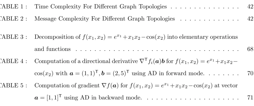
TABLE 1 : Time Complexity For Different Graph Topologies . . . 42

TABLE 2 : Message Complexity For Different Graph Topologies . . . 42

TABLE 3 : Decomposition off(x1, x2) =ex1+x1x2−cos(x2) into elementary operations

and functions . . . 68

TABLE 4 : Computation of a directional derivative∇T_f

i(a)bforf(x1, x2) =ex1+x1x2−

cos(x2) witha= (1,1)T,b= (2,5)Tusing AD in forward mode. . . 70

TABLE 5 : Computation of gradient∇f(a) forf(x1, x2) =ex1+x1x2−cos(x2) at vector

LIST OF ILLUSTRATIONS

FIGURE 1 : Path graphP8 . . . 37

FIGURE 2 : Grid GraphGG4×8. . . 37

FIGURE 3 : Ring graphR8 . . . 38

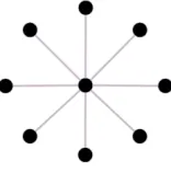
FIGURE 4 : Star graph_S9 . . . 38

FIGURE 5 : Erdos-Renyi graphERn,pwithp= 0.1 andp= 0.2 . . . 39

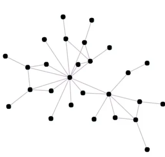
FIGURE 6 : Scale Free NetworkSFn . . . 40

FIGURE 7 : Bar Bell GraphBBG8 . . . 41

FIGURE 8 : Ramanujan Expander GraphREG3,20 . . . 42

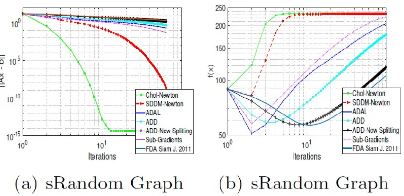
FIGURE 9 : Experimental Results for Small Random Graph . . . 53

FIGURE 10 : Experimental Results for Large Random Graph . . . 53

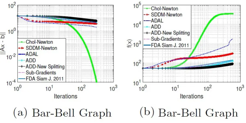
FIGURE 11 : Experimental Results for Bar-Bell Graph . . . 54

FIGURE 12 : Experimental Results for Bar-Star Graph . . . 54

FIGURE 13 : Experimental results: convergence, communication overhead, accuracy effect 55 FIGURE 14 : Computational graph forf(x1, x2) =ex1+x1x2−cos(x2) . . . 69

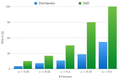
FIGURE 15 : The effect of dimensionality using Automatic Differentiation . . . 72

FIGURE 16 : The effect of dimensionality. . . 85

FIGURE 17 : SPARK computational model. . . 86

FIGURE 18 : The effect of dimensionality for the SPARK model . . . 87

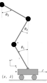
FIGURE 19 : Double Cart Pole System . . . 89

FIGURE 20 : Experimental Results on Linear Regression with a synthetic data set. . . . 90

FIGURE 21 : Experimental Results on Linear Regression with a real data set. . . 90

FIGURE 22 : Experimental Results on Logistic Regression with L2regularization. . . 91

FIGURE 23 : Experimental Results on Logistic Regression with L1regularization. . . 91

FIGURE 24 : Experimental Results on Reinforcement Learning. . . 92

FIGURE 25 : Experimental Results on fMRI images. . . 93

FIGURE 26 : Experimental results: communication overhead, CPU running times . . . . 94

FIGURE 28 : Experimental Results for Large Random Graph . . . 129

FIGURE 29 : Experimental Results for Bar-Bell Graph . . . 130

FIGURE 30 : Experimental Results for Bar-Star Graph . . . 131

FIGURE 31 : Experimental results: convergence, communication overhead, accuracy effect 132 FIGURE 32 : Experimental Results on Linear Regression with a synthetic data set. . . . 133

FIGURE 33 : Experimental Results on Linear Regression with a real data set. . . 134

FIGURE 34 : Experimental Results on Logistic Regression with L2regularization. . . 135

FIGURE 35 : Experimental Results on Logistic Regression with L1regularization. . . 136

FIGURE 36 : Experimental Results on Reinforcement Learning. . . 137

FIGURE 37 : Experimental Results on fMRI images. . . 138

FIGURE 38 : Experimental results: communication overhead, CPU running times . . . . 139

FIGURE 39 : Computational binary tree for ΦT_{(b)x . . . . 140}

FIGURE 40 : Computational graphGgi forgi(x). Input nodes are marked by green. Last node is marked by red. . . 140

CHAPTER 1 : INTRODUCTION

Data analysis has become a major tool for acquiring predictive models with the goal of discovering

useful information, suggesting conclusions, and supporting decision-making in a variety of fields

including but not limited to heath-care (Zupan et al. (1997)), engineering (Spiliopoulou et al. (2014)),

marketing (Jeffery (2010)), et cetera. Before achieving a ”data product” raw information has to go

through several phases. After being acquired, data is first processed and cleaned to remove errors

and record duplication, as well as to recognize outliers that might have been incorrectly entered.

Once cleaned, it can be analyzed to arrive at mathematical models that can be used to derive

conclusions and make predictions in reality. The goal of such models is to identify relationships

among the variables, such as correlation or causation that reflect inherent properties in a particular

data set. Machine learning (ML) is a sub-field of computer science that is dedicated to deriving these

complex predictive models. In ML, computers act without being explicitly programmed. Contrary

to standard programming paradigms, in ML, a programmer designs a general architecture of a

computer code that can accept inputs and derive outputs. Rather than pre-setting all required

parameters to achieve the desired task, these are acquired with the aid of input data through a

process of self-tuning. Here the program automatically optimizes for free-parameters to minimize a

cost function that describes the task. To clarify, consider the example of classifying images of rhinos

versus elephants. A general computer program that can accept images, say in pixel format, and

output a class label, i.e., a discretized zero/one output, is first written. The program, however, is not

explicitly told how to output a class label to an input image. Rather a form of parameterized mapping

between images and class labels is assumed (e.g., logistic function, neural network, etc.). Having

acquired data, self-tuning commences to determine the ”best” parameters (i.e., those that optimize

a pre-specified cost/error on the training data) that correctly classifies rhinos from elephants.

Searching for the ”best” set of free-parameters ties machine learning to numerical optimization, which

delivers a rich literature of efficient and scalable algorithms for data analysis and machine learning.

Among these, maybe the most abundant are centralized first-order gradient techniques ( Boyd and

Vandenberghe (2004b), Ruder (2016), Andrychowicz et al. (2016a)). These algorithms come in

different flavors under different names, including gradient and steepest descent ( Andrychowicz et al.

following a scaled version of the gradient of the cost function. In the standard case, the gradient

is computed by running over all data points, while in the stochastic setting only one or a subset of

the data is considered, leading to a more appealing algorithm for large-scale applications. Though

abundant and cheap to compute, stochastic gradient-based methods are relatively slow exhibiting

sub-linear convergence of the formO_√1

t

withtbeing the total number of iterations ( Blair (1985),

Agarwal et al. (2012)). This performance is caused by the diminishing step size essential for the

global convergence. Adaptive Gradient (AdaGrad) is an alternative approach that removes the

step size issue by dynamically incorporating knowledge of the geometry of the data observed in

earlier iterations to perform more informative gradient-based learning. In other words, this method

gives frequently occurring features low learning rates and infrequent features high learning rates. The

intuition behind of this behavior is that each time an infrequent feature is seen, the algorithm should

take notice. Thus, the adaptation facilitates finding and identifying very predictive but comparatively

rare features ( Duchi et al. (2010)). Although the convergence properties of AgaGrad are similar to

to those of its stochastic counterpart, numerous empirical studies show significant improvement for

the sparse data set scenarios.

Aiming at improving convergence speed limitations, the authors in Boyd et al. (2011) relied on

a primal-dual decomposition technique to propose the alternating direction method of multipliers

(ADMM) that achieves linear convergence of the formO 1

t

. Despite being successful at efficiently

reducing the error function value, it has been shown in later studies ( Nishihara et al. (2015),

Kadkhodaie et al. (2015)) that ADMM requires numerous iterations to achieve accurate solutions.

Another class of algorithms with superior performance to these detailed earlier is the class of

second-order (Newton) methods. Rather than solely relying on the gradient, Newton iterates consider the

curvature of the optimization objective by taking Hessian (the matrix of second-order gradients)

into account. Here, updates are done by descending in the Newton direction. Convergence results

in Boyd et al. (2011) have shown that following the Newton direction leads to improved algorithms

with two phases of convergence being strict and quadratic decrease. Despite the fast convergence

properties, the centralized application of Newton method is restricted by the necessity to compute

and invert the Hessian matrix. This situation becomes even worse for large-scale scenarios due to

excessive memory requirements.

Recently, researchers and developers have met new computational challenges caused by a remarkable

are growing much faster than processing speeds, making traditional centralized solutions (such as

various first order stochastic gradient descent (SGD) algorithms) inefficient. As an example let us

consider the current state of the art deep neural networks ( Szegedy et al. (2015), Krizhevsky et al.

(2012)) operating with millions of parameters and characterizing with a very slow training time

(may take several days). The typical strategy to accelerate the training procedure is adopting it to a

parallel framework by allocating resources over many machines. (Dean et al. (2012)). This approach

not only speeds up neural network training but also allows researchers to build more sophisticated

models where different machines compute different splits of the mini-batches. Even though SGD

exhibits nice scalability with respect to the complexity of a model and the size of datasets, it does

not adopt well into a parallel setting: larger mini-batches and more parallel computations exhibit

diminishing returns for SGD algorithms.

In the past decades, distributed programming frameworks such as Open Message Passing Interface

(MPI) have endorsed rich primitives to leverage flexibility in implementing algorithms across

dis-tributed computing resources, often delivering high-performance but coming with the cost of high

implementation complexity ( Quinn (2003)). Despite the high performance and significant practical

impact, the large-scale application of MPI methods is restricted by implementation complexities. In

order to handle correctly communication and synchronization between clusters, MPI methods require

a lot of programming effort as well as deep system-level understanding. The alternative models, such

as Hadoop and SPARK, have recently emerged and formulated well-defined distributed

program-ming paradigms leading to a powerful set of APIs specially built for distributed processing ( Chu

et al. (2007)). These abstractions make the implementation of distributed algorithms more easily

accessible to researchers, but seem to come with poorly understood overheads associated with

com-munication and data management, which make the tight control of computation vs comcom-munication

cost more difficult.

Apart from serving as a computational tool for very specialized scientific purposes and companies’

operational routines, distributed optimization is strongly involved in new emerging global

technolo-gies, such as Internet of Things (IoT) ( Vermesan and Friess, Mattern and Floerkemeier (2010)).

Simply put, IoT is the concept of connecting basically any device with an on and off switch to the

Internet (and/or to each other). Cell phones, headphones, lamps, refrigerators, coffee machines and

giant network of connected intelligent components interacting with each other. The analyst company

Gartner predicts that by 2020 the number of components in this network will be over 26 billion.

According to the recent EU Commission action plan recognized the Internet of Things as a general

evolution of the Internet from a network of interconnected computers to a network of interconnected

objects” ( IoT (2009)).

From a technical point of view, the IoT is not the result of a single novel technology; instead, several

complementary technical developments provide capabilities to build a bridge between the virtual

and physical world. These capabilities include but are not limited to:

• Communication and cooperation: Different components of the IoT network have the ability

to interact with each other, to make use of data and services and update their state. Wireless

technologies such as WPAN, GSM and UMTS, Wi-Fi, Bluetooth, ZigBee and various other

wireless networking standards are currently under development.

• Distributed information processing: Intelligent objects feature a processor, plus storage

capac-ity. These resources can be used, for example, to process and interpret sensor information, or

to collectively perform more sophisticated computations.

IoTs distributed and dynamic nature, resource constraints of sensors and embedded devices as

well as the amounts of generated data are challenging even for the most advanced data analysis

methods known today. In particular, the IoT requires a new generation of distributed analysis

methods. Many surveys ( Atzori et al. (2010), Gubbi et al. (2013) Partynski and Koo (2013),

Xu et al. (2014)) have strongly focused on the centralization of data in the cloud and big data

analysis (so-called Master/Slave model), which follows the paradigm of parallel high-performance

computing. However, bandwidth and energy can be too limited for the transmission of raw data,

or it is prohibited due to privacy constraints. Such communication-constrained scenarios require

decentralized analysis algorithms which at least partly work directly on the generating devices.

In the distributed setting, central problems are split across multiple processors each having access

to local objectives. To clarify, consider our running example of classifying images of rhinos versus

elephants. Rather than searching for a centralized solution, one can distribute the optimization

across multiple processors each having access to local costs defined over random subsets of the full

unified by incorporating consensus constraints. Recently, an increasing body of research has targeted

such a setting explicitly. For instance, Google’s federated learning aims at achieving collaborative

model learning across multiple mobile devices without the need for centralized training data in the

cloud. Here, a unified model is learned collaboratively based on only local data available on each

mobile device (Konecn´y et al. (2016b), Konecn´y et al. (2016a)). Another example of the growing

trend for distributed optimization is the recent work of McMahan et al. (2016). Here, the authors

consider highly-dimensional optimization problems with billions of parameters and solve them with

the help of tens of thousands of CPU cores. They show that this approach can lead to improved

convergence allowing for algorithms that can handle such Big Data problems.

Analogous to the centralized literature, distributed optimization has also provided a rich set of

al-gorithms for determining free parameters in a decentralized fashion by relying on communication

between the involved processors. Among many approaches (e.g., distributed averaging ( Olshevsky

(2014)), coordinate descent ( Richt´arik and Tak´ac (2013), Trofimov and Genkin (2015)) and

incre-mental methods ( Bertsekas (2015), Nedic et al. (2001)), two popular classes can be differentiated.

The first is sub-gradient based, while the second relies on a decomposition-coordination procedure.

Sub-gradient algorithms are similar to centralized first-order gradient methods, where they proceed

by taking a gradient-related step, followed by an averaging with the neighbors at each iteration.

The computation of each step is relatively cheap and can easily be implemented in a distributed

fashion ( Nedic and Ozdaglar (2009)). Though cheap to compute, the best known bound on the

rate of sub-gradients is sub-linear. As such, these algorithms share the problems of their

central-ized counterparts. The second class of algorithms solve constrained problems by relying on dual

methods. Their state-of-the-art technique is a distributed version of the centralized ADMM ( Wei

and Ozdaglar (2012), Chang et al. (2015)) that achieves a linear convergence rate with low message

complexity per iteration. Apart from only achieving linear convergence, distributed ADMM has also

been shown to suffer from accuracy issues as detailed in Kadkhodaie et al. (2015).

Many rate and accuracy improvements can be gained from adopting distributed second-order

(New-ton) methods. Though a variety of techniques have been proposed (Zargham et al. (2013) Mokhtari

et al. (2015), Gurbuzbalaban et al. (2015), Eisen et al. (2016)), less progress has been made at

leveraging ADMM’s accuracy and convergence rate issues.

by using the approach in Zargham et al. (2013) to approximate the Newton direction. As detailed

later, this method suffers from two problems. First, it fails to outperform ADMM and second, it

faces storage and computational deficiencies for large data sets, and thus ADMM retains

state-of-the-art status.

The alternative approach proposed by Eisen et al. (2016) calculates Newton direction by applying

a distributed version of the Sherman-Morrison formula ( Sherman and Morison (1949)). The

advan-tages of D-BFGS relative to approximate Newton methods are that they do not require computation

of Hessians, which can itself be expensive, and that they apply in any scenario in which gradients

are distributedly computable irrespective of the structure of the Hessian. In terms of convergence

properties, D-BFGS resembles the previously discussed Network Newton algorithm and empirically

surpassed by ADMM.

In scenarios where the number of local functions is large and not all of them simultaneously

avail-able, one is interested in optimization techniques that can iteratively update the estimate for an

optimal solution using partial information about component functions. The incremental Newton

method ( Gurbuzbalaban et al. (2015)) cycles deterministically through the component functionsfi

and uses the gradient offito determine the descent direction and the Hessian offito construct the

Hessian of the sum of component functions. Apart from requiring a global coordinator, this method

suffers from immense computational requirements caused by sequential inversion of local Hessians

in each iteration.

Contributions: In the previous paragraphs we discussed a general distributed optimization

frame-work and presented a brief overview of existing decentralized algorithms. In the next paragraphs,

we focus on both theoretical and practical contributions of this thesis.

Though appealing, computing the Newton direction in a distributed fashion is challenging due to

the need of inverting the Hessian matrix that requires global information. In our work, a novel

connection between the Hessian of a distributed optimization problem and Symmetric Diagonally

Dominant (SDD) matrices is derived. Recently, SDD matrices have captured strong attention due to

a series of breakthrough results (Koutis and Miller (2007), Kelner and Madry (2009), Kelner et al.

(2013), Cohen et al.) starting with work of Daniel Spielman and Shang-Hua Teng ( Spielman and

Teng (2006)) who suggested the first almost linear time algorithm for solving SDD linear systems.

domi-nance property gives us hope to calculate the Newton direction for a distributed problem without a

heavy computational burden by attempting fast distributed SDD solvers.

In Section 2.2 we suggested two fully distributed algorithms for solving symmetric diagonally

dom-inant systems. The first method utilizes the idea of Peng and Spielman (2013) by constructing

decentralized approximated inverse chain in a recursive fashion. This chain can be visualized as a

collection of matrices such that each cluster stores only the corresponding row of each of these

ma-trices. By traversing this chain first in forward and then in backward direction we arrive at a crude

solution of the SDD system that approximates an exact solution up to some constant accuracy. In

order to reach any given precision, we accompany the approximated inverse chain with an iterative

procedure called Richardson Preconditioners ( Axelsson (1994a)) gradually improving the accuracy.

To the moment of publishing, this method was the fastest fully distributed SDD solvers with time

complexity proportional to a condition number of an SDD matrix.

The linear dependence on a condition number is favorable for a wide range of cluster topologies

including expanders ( Hoory et al. (2006)), random graphs ( Hofstad (2008)), and grids ( Fadel et al.

(2015)). However, for configurations of clusters characterized by long diameters this behavior might

lead to a slow performance. As an example, let us consider BarBell topology for clusters ( Northup)

where two cliques of size dn

3e connected with a path graph on d

n

3e nodes. Due to this bottleneck

part, the corresponding condition number for SDD matrices can be cubic in a number of clusters.

To remedy this effect consider a polynomial approximation of SDD inverse with properly scaled

Chebyshev polynomials. The particular choice of these polynomials is motivated by their extremal

properties and the fast performance of the algorithm is guaranteed by the recursive relation between

them ( Chebyshev (1853)). Eventually, we arrive at a new SDD solver capable of computing an

approximate solution with any given precision in time proportional to the square root of a condition

number of an SDD matrix.

Having introduced fully decentralized techniques, we noticed that the total number of messages (in

literature often referred to as communication complexity) is increasing with ”spreadness” of the

underlying network of clusters. To illustrate this phenomenon, let us consider Star Graph ( Shao

et al. (2000)) and previously discussed Barr-Bell models. In the former, all nodes are only

con-nected to a single master node responsible for all computational burden. As a result, the message

complexity in this case is only characterized by the number of clusters n. In the latter model, the

message complexity to be bounded byOn72

. Therefore, the question that follows naturally from

this observation is: can we eliminate this drastic effect of cluster configuration by ”slightly” relaxing

the decentralization requirements. Please notice, that by completely removing this requirement we

arrive at a highly impractical scenario, where all input data must be stored and processed in a single

cluster. In Section 2.3, using spectral sparsifiers, we propose a mixed strategy that allows for a fixed

node to aggregate some information from all others while preserving the slightly worse bound on

the size of local memory of this cluster compared to the fully decentralized case. Surprisingly, apart

from significantly improving the message complexity, we show that the time complexity of a new

mixed algorithm is even faster than in centralized and fully decentralized scenarios.

On the practical side, we contribute by applying the proposed SDD solvers for two problems that

have been in the focus of researchers for many years: Network Flow Problems and Empirical Risk

Minimization.

Network Flow Problems are considered one of the most fundamental problems in industrial

engen-dering and theoretical computer science ( Ahuja et al. (1993b), Ford and Fulkerson (2010), Dahan

and Amin (2016), Aly and Van Vyve (2015)). The ultimate goal here is to minimize the total cost

associated with all edges connecting clusters subject to flow conservation constraints. In Section 3.1

we show that significant progress can be attained by applying primal-dual techniques and

formu-lating an unconstrained dual problem. Careful analysis of the dual function shows that its Hessian

exhibits diagonal dominant property and, therefore, concedes utilization of SDD solvers for

calculat-ing the correspondent Newton direction. As a result, we develop the first exact distributed Newton

method for Network Flow problem demonstrating a quadratic convergence rate. We empirically

validate this result on a variety of numerical simulations with real data against several methods,

including the state-of-the-art ADAL algorithm (Chatzipanagiotis et al. (2015)).

Our second practical contribution is motivated by machine and statistical learning and has a wide

range of applications in data science ( Zhang (2010)), robotics ( Cetto et al. (2013)), image

pro-cessing ( He et al. (2015)), speech recognition ( Yu and Deng (2014)) et cetera. In Empirical Risk

Minimization problem a true risk defined by the unknown probability distribution over the training

func-tions computed at each data point for the chosen prediction model. In the distributed framework

the associated optimization problem is formulated as a finite sum minimization problem combined

with consensus constraints between the clusters. In Section 3.2.9, following primal-dual strategy

we constructed the corresponding dual function and recognize that its Hessian can be represented

as a product of SDD matrices. Based on this observation we calculate the Newton direction by

sequentially solving a collection of SDD systems. Our exact distributed Newton method for the

Empirical Risk Minimization problem is the first distributed algorithm achieving a quadratic

con-vergence rate. Finally, we suggest Hessian-free and stochastic variation of our algorithm by applying

automatic differentiation techniques and the Sherman-Morrison formula. In Section 3.2.9 we verify

our superior performance by conducting a series of numerical simulations:

• against traditional decentralized stochastic gradient descent method using SPARK.

• against centralized stochastic gradient descent using streaming.

• against other distributed algorithms including state-of-the-art distributed ADMM (Wei and

Ozdaglar (2012))

CHAPTER 2 : SYMMETRIC DIAGONAL DOMINANT SOLVERS

The problem of solving a system of linear equations given by symmetric diagonally dominant

ma-trices (SDD) arises in a variety of real-world applications. For example, SDDs appear in multitude

of fields including but not limited to determining solutions of partial differential equations

LeV-eque (2007), semi-supervised learning Zhu et al. (2003), Zhou and Schlkopf (2004), computer vision

Casaca (2015), and computation of maximum flows in graphs Daitch and Spielman (2008), Madry

(2013).

Recently, much progress towards solving such problems has been made. Out of the different

tech-niques, the solution of Speilman and Teng Spielman and Teng (2006) stands out. Here, the authors

exploited three components for an efficient SDD solver. Namely, using the multi-level framework

suggested by Joshi (1996), low-stretch spanning tree preconditioners introduced by Boman et al.

(2008), and spectral graph sparsifiers Spielman and Teng (2008), they proposed a nearly linear-time

algorithm for solving SDD systems. These results were then improved by Koutis et al. Koutis et al.

(2010), Cohen et al. (2014), who developed an even faster algorithm for acquiring-close solutions to

SDD linear systems. Improvements have since been discovered by Kelner et al. Kelner and Madry

(2009), where their algorithm relied on only low stretch trees and eliminated the need for graph

sparsifiers and the multi-level framework.

Motivated by applications, much interest has been devoted to developing parallel versions of these

algorithms. Koutis and Miller Koutis and Miller (2007) proposed an algorithm requiring

nearly-linear work and m16 depth (m is the total number of nonzero entries of SDD matrix) for planar

graphs. This result was then extended to general graphs in Blelloch et al. (2011) leading to depth

close to m13. Since then, Peng and Spielman Peng and Spielman (2013) have proposed an efficient

parallel solver requiring nearly-linear work and poly-logarithmic depth without the need for

low-stretch spanning trees.

Less progress, on the other hand, has been made in the distributed version of these solvers. Contrary

to the parallel setting, memory is not shared and is rather distributed in the sense that each unit

Bertsekas and Tsitsiklis (1989) can be used for such distributed solutions but require substantial

complexity. In Mou et al. (2015), the authors propose a gossiping framework for acquiring a

solu-tion to SDD systems in a distributed fashion. Recent work Lee et al. (2014) considers a local and

asynchronous solution for solving systems of linear equations, where they acquire a bound on the

number of needed multiplication proportional to the degree and condition number of the graph for

one component of the solution vector.

In this chapter, we target both the theoretical investigation of distributed SDD solvers, as well

as their practical applications. The first part of the work provides basic definitions and properties

of SDD systems and then presents three fully distributed and one mixed algorithm for solving SDD

systems in a decentralized fashion. For all proposed methods we analyze the running time and

communication complexity in terms of the underlying graph topology. Finally, to provide better

intuition, we consider the following special cases for the processors’ graphs: path graph, grid graph,

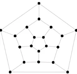
ring graph, random graph, scale-free network, barbell graph, and Ramanujan expander.

The second part of the work includes interesting practical applications. In Section 3.1, we

con-sider network flow optimization - a fundamental problem with wide-ranging applicability including

but not limited to, DNA sequence alignment Ahuja et al. (1993a), scheduling on uniform parallel

machines Lawler et al. (1982), urban traffic flows Ahuja et al. (1993a), optimal energy allocation

Gurakan et al. (2015), etc. As networks grow larger, centralized approaches to network flow

op-timization underperform due to the increase in time and resource complexity needed. Distributed

methods for such network optimization problems present an alternative direction to cope with such

increased demand. Since existing distributed methods exhibit slow convergence rate (at most linear),

we propose a fully decentralized version of the Newton method using the developed SDD solvers

to arrive at quadratic convergence. On the empirical side, we demonstrate that our method

out-performs current algorithms for network flow in a broad set of experiments on a variety of network

topologies. We also show that this outperformance arrives at no increase in the local communication

2.1. Preliminaries

Throughout the remainder of this thesis we letG= (V,E,W) be a weighted connected undirected

graph with |V| = n nodes and E edges. We also assume that we > 0 for all e ∈ E. Each node

i∈Vrepresents an agent which is capable of storing information in local memory and can perform

computations. Moreover, the size of local memory for each node is bounded by O(n) making it

impossible to gather the full topology of network_Gin one node. The distributed symmetric diagonal

dominant system associated with_Gis given as:

L_Gx=b (2.1)

whereL_G∈Rn×n such that

L_G(ij) = 0, ∀(i, j)6∈E

|L_G(ii)| ≥ −

n X

j=1

|L_G(ij)| ∀(i)∈V

Due to the sparsity pattern ofL_G, Equation (2.1) can be represented in distributed fashion among

the nodes of G. Particularly, each node i ∈ G stores LG(ij) for j = 1, . . . , n, as well as the i

th

component, i.e.,b(i), of the demand vectorb. The goal is for each node to compute the corresponding

component of the solution vector by only allowing local message exchange between the nodes. As a

straightforward example of (2.1) is a Laplacian system, where

L_G(ij) =



    

    

P

e∼iwe :i=j

−we : (ij)∈E

0 :otherwise

Following Koutis et al. (2010), we target an−close solution of the system in 2.1, which is defined

as:

Definition Letx∗ be the exact solution of system L_Gx=b. A vector ˜x is called approximate

solution, if

||x˜−x∗||LG≤||x

∗_||

where||u||2 LG=u

T_L Gu.

The important characteristic of system (2.1), which will be heavily used in our analysis is the

condition number, defined as:

Definition Let{µi}pi=1 be the collection of all non-zero eigenvalues of matrixLG, such that

µ1≤µ2≤. . .≤µp

The the ratioκ(L_G) =µp

µ1 is called condition number of system (2.1).

In the case of graph Laplacians κ(L_G) = µn

µ2 ≤

1 2

wmax

wminndmaxdiam(G), wherewmax, wmin are the

maximal and minimal edge weights in_G,diam(_G) its diameter, anddmaxis the maximal unweighted

degree.

Finally, we assume a synchronous model for distributed computation. Here, all message exchanges

between the nodes as well as local operations are directed by a global clock. The time complexity

is given in terms of the total number of time steps on the global clock needed to terminate an

algorithm. The message complexity (or communication complexity) is given in terms of the total

number of messages sent by nodes to terminate an algorithm.

2.2. Fully Distributed Methods

In this section, we describe two fully distributed algorithms for solving the system in (2.1). We

commence by describing the algorithms and then study their time and communication complexities.

2.2.1. Algorithm I: Matrix Inverse Chain Approach

The authors in Peng and Spielman (2013) developed a near-linear time solver capable of achieving

an−close approximation to the exact solution for any arbitrary >0. In this section, we propose

a distributed implementation of the aforementioned solver. Before presenting our solver, however,

Standard Splitting and Approximations

The story of computing an approximation to the exact solution of an SDD system of linear equations

starts from the standard splitting of symmetric matrices. Given a symmetric matrixL_Gthe standard

splitting is given by

L_G=D0−A0 (2.3)

where D0 is a diagonal matrix that consists of the diagonal elements in LG while A0 is a matrix

collecting the negate of the off-diagonal components inL_G. As the goal is to determine a solution

of the SDD system, we will be interested in inverses ofL_G. Given the splitting in Equation 2.3, the

authors in Peng and Spielman (2013) prove that the inverse ofL_G can be written as

(D0−A0)−1= 1 2

h

D−₀1+ I+D−₀1A0

D0−A0D−₀1A0−1

I+A0D−₀1i

(2.4)

SinceD0−A0D−₀1A0 is also SDD we can recurse the above for the length ofd=O(logn) to arrive

at the so-called inverse approximated chain,C={Dk,Ak}dk=1with

Dk=D0 and Ak=D0 D−01A0 2k

(2.5)

Hence, the inverse at thekth_{recursion can be written as}

(Dk−Ak)−1≈

1 2

h

D−_k1+ I+D−_k1Ak(Dk+1−Ak+1)−1 I+AkD−k1 i

Algorithm 1: ”Crude” SDD Solver

1: Input: Inverse approximated chainC, demand vector b. 2: Output: A ”crude” approximationx0 to the exact solutionx∗.

3: Initialize: b0=b.

4: fork= 1 tod=O(logn)do

5: bk= I+Ak−1D−k−11

bk−1.

6: end for

7: xd=D−_d1bd.

8: fork=d−1 to 0do

9: xk= 1₂D−k1bk+ I+D−k1Akxk+1.

10: end for

Given the above, the approximate solution to the SDD system can be achieved using a two-step

Algorithm 1 describes a set of instructions used to acquire a crude approximation to the real solution

of the SDD system. The algorithm runs a forward and a backward loop with the number of steps

equal to the length of the inverse approximate chaind1_{. In the forward loop (lines 4-6) intermediate}

vectors are constructed and used in the backward loop (lines 8-10) to determine a constant error (see

2.1) solution to the exact solution of the SDD system. Since the approximation incurs a constant

error to the real inverseL−1

G , the authors in Peng and Spielman (2013) then introduce the Richardson

preconditioning scheme detailed in Algorithm 2 to arrive at any arbitrary precision

Algorithm 2: ”Exact” SDD Solver

1: Input: Inverse approximated chainC, demand vector b, precision parameter.

2: Output: −close approximation ˜x, to the exact solutionx∗.

3: Initializey₀=0.

4: Setχto be the crude solution returned by Algorithm 1.

5: fork= 1 tod=O log1

do

6: Setu(1)_k =L_Gy_k−1.

7: Setu(2)_k by calling Algorithm 1 with b=u(1)_k .

8: Updatey_k=y_k−1−u(2)_k +chi

9: end for

10: Set ˜x=y_q.

Algorithm 2 uses Algorithm 1 as a sub-routine to drive the ”crude”-solution to−close approximate

one for any >0 inO log1iterations.

The authors in Peng and Spielman (2013) show that the above iteration scheme can be parallelized

across multiple processors leading to an algorithm which can acquire -approximate solutions in

nearly linear time. As our goal is to determine the Newton direction of network flow problems in a

distributed fashion, i.e., using only local information exchange, we next present a distributed version

of Algorithms 1 and 2. Our strategy is similar to that in Peng and Spielman (2013) with crucial

differences related to the type and length of the inverse approximate chains as detailed below.

Distributed SDD Solvers: Methodology

A key ingredient enabling efficient solvers for SDD systems is the introduction of the inverse

approx-imate chain which rendered a parallelized implementation. Since our interest lies in a distributed

solution for determining the Newton direction, the first step needed for the development of our SDD

solver is an inverse chain which can be computed in a distributed fashion using only local

nication exchange among the nodes of G. As noted in Peng and Spielman (2013), a collection of

matricesC={D0,A0. . . ,Dd,Ad}is an inverse approximate chain toLGif there exist positive real

numbers0, . . . , d such that the following three conditions are satisfied:

1. Dk−Ak ≈k−1 Dk−1−Ak−1D −1

k−1Ak−1, for allk={1, . . . , d}.

2. Dk≈k−1 Dk−1 and

3. Dd≈dDd−Ad.

The ”≈” defines the notion of approximation for matrices previously introduced in Peng and

Spiel-man (2013) whereX≈Y is written to indicate

exp(−)XY exp()X

whereX Y reflects thatX−Y is positive semidefinite.

Starting from L_G = D0−A0, and defining the inverse chain as in Equation 2.5, it is easy to

verify thatC is an inverse approximate chain toL_G as it satisfies all three of the above conditions.

Hence, it can be used for computing a crude solution to an SDD system. To derive the distributed

algorithm, we further examine the update equations of Algorithm 1. Studying the forward loop, the

intermediate vectorsbk are constructed according to

bk= I+Ak−1D−k−11

bk−1=bk−1+A0D0−1A0D−01. . .A0D−01

| {z }

a product of 2k_matrices

bk−1

Examining each product of the 2k _{matrices, e.g., A0D}−1

0 A0b0, we recognize that such a product

can be computed locally by each node. This is true as the first part of the product, i.e.,z=D−₀1b0

is a simple scaling, while the second, i.e.,A0zcan be performed completely in a distributed fashion

due to the sparsity pattern ofA0. Consequently, the overall product of the 2k terms can be also

distributed across the network provided the usage of a recursive update rule. Therefore, for a node

i, the first part (i.e., forward loop) of the distributed solver can be concisely summarized using the

set of instructions detailed in Algorithm 3.

Clearly, lines 6-8 are executing the distributed computation of the product of the 2kterms above,

while line 9 of the algorithm is computing theith_{component ofb}

de-scribed above. After running for a total ofditerations, Algorithm 3 returns theithcomponent of

in-termediate vectorsb1, . . . ,bd. Further, since the length of the chaind=dlog

2 ln 3 √

2

3 √

2−1

_w

max

wminn 3_e

withwmaxandwmindenoting the largest and smallest edge weights, each node needs to have memory

size ofO(max{d, dmax}) =O(n).

Algorithm 3: Forward Loop: Distributed ”Crude” Solver

1: Input: The ith row of matrices A0,D0, the ith component of vector b, the length d =

dlog2 ln 3 √

2

3 √

2−1

wmax

wminn

3_{eof approximated inverse chain.}

2: Output: Theith_{components of vectorsb1, . . . ,b} d.

3: fork= 1 toddo

4: Setl= 2k−1_.

5: Updatehu(₁k−1)i

i

=

A0D−₀1bk−1_i.

6: forj= 2 toldo

7: Updatehu(_jk−1)i

i= h

A0D−₀1u(_jk₋−₁1)i

i.

8: end for

9: Set [bk]i= [bk−1]i− h

u(_lk−1)i

i

.

10: end for

1

Analogous to Algorithm 1, the distributed solver commences by running a backward loop to compute

theith_{component of the crude solution [x0]}

i. Using a similar analysis to that of the forward rule, the

recursive update equations are represented in Algorithm 4. Algorithm 4 distributes the computations

of the products involved in determining theithcomponent of x0 using recursion. Furthermore, it

uses the same chain length as that in Algorithm 3.

Algorithm 4: Backward Loop: Distributed ”Crude” Solver

1: Input: The ith _{row of matrices A}

0,D0, the ith component of vector b, the length d = dlog2 ln 3

√ 2

3 √

2−1

wmax

wminn

3_{eof approximated inverse chain, and [b}

d]i as returned by Algorithm

3.

2: Output: Theithcomponents of ”crude” solution [x0]i.

3: Set [xd]i= _[D[bd]i

0]ii

4: fork=d−1 to 1do

5: Setl= 2k. 6: Updatehη(₁k+1)i

i

=

D−₀1A0xk+1

i.

7: forj= 2 toldo

8: Updatehη(_jk+1)i

i

=hD−₀1A0η (k+1)

j−1 i

i

.

9: end for

10: Set [xk]i =1₂ h _[b

k]i

[D0]ii + [xk+1]i+

h η(_lk+1)i

i i

.

11: end for

12: Set [x0]i= 1₂ h _[b]

i

[D0]ii+ [x1]i+

D−₀1A0x1 i

Having developed an algorithm which computes a crude approximation to an SDD system of linear

equations, we now provide an exact distributed solver which can drive x0 to an -close solution

for any arbitrary > 0. Similar to the previous analysis, each node i receives the ith _{row of}

L_G, the ith _{component of the right-hand side vector [b]}

i, the length of the inverse chain d, and a

precision parameter as inputs. The algorithm then determines the ith _{component of the -close}

approximation to the real solutionx∗as detailed in Algorithm 5. It should be noted that Algorithm

5 is a simple distributed implementation of the Exact SDD solver, where the products are computed

locally based on the sparsity pattern ofL_G.

Algorithm 5: ”Exact” Distributed SDD Solver

1: Input: Theith_{row of matricesA}

0,D0, theithcomponent of vectorb, precision parameter.

2: Output: Theith_{components of−approximate solution [˜x]} i.

3: Initialize: [y₀]i= 0 and [χ]i by running Algorithms 3 and 4 with [A0]i1, . . . ,[A0]in,[D0]ii,[b]i

anddas inputs.

4: fort= 1 toq=O 1

do

5: Sethu(1)_t i

i

=

L_Gy_t−1 i.

6: Set hu(2)_t i

i

by running Algorithms 3 and 4 with [A0]i1, . . . ,[A0]in,[D0]ii,[u

(1)

t ]i and d as

inputs.

7: Update [yt]i= [yt−1]i− h

u(2)t i

i+ [χ]i.

8: end for

9: Set [˜x]i= [yq]i

Having developed the solvers, we next illustrate the most important theoretical results attained by

our distributed SDD solver and compare to current literature.

Theoretical Guarantees

In this section, we provide theoretical justification for the correctness of Algorithm 5. Namely, we

show that the distributed solver is capable of acquiring-close approximations to the exact solution

of the SDD system and provide its iteration count in terms of the network’s properties. These results

are summarized in the following theorem:

Theorem 2.2.1 The distributed SDD solver described in Algorithm 5 uses local communication

exchange to compute an-approximate solution of the SDD systemL_Gx=bin the following number

of rounds

O

κ(L_G)wmax wmin

log

1

whereκ(L_G)is condition number ofG, andwmax, wmin are maximal and minimum edge weights.

To arrive at such results, we require the analysis of both the crude and the exact distributed SDD

solvers. The remainder of this section is dedicated to the proof of the above theorem. It proceeds by

presenting two essential lemmas. The first shows that the distributed crude solver (i.e., Algorithms 3

and 4) returns a constant error approximation to the exact solution of the SDD system. The second

demonstrates that the exact solver in Algorithm 5 drives the crude solution to an-close one and

provides its iteration count.

To arrive at a crude approximation to the real solution of the SDD system, we need to show that

the procedure described in Algorithms 3 and 4 is capable of approximating the inverse of L_G and

providing a good enough approximation to the exact solution. The accuracy of this approximation

and the needed iteration count has also to be quantified. We summarize these results for the case

of graph LaplacianL_G in the following

Lemma 2.2.2 Let L_G =D0−A0 be the standard splitting. Let the length of the inverse chain is

defined as d=dlog2 ln 3 √

2

3 √

2−1

wmax

wminn

3_{e. Further, let Z}0 _{be the operator defined by the ”crude”}

solver, such thatx0=Z0b. Then

1. d <1₃ln 2.

2. Z0≈dL −1

G , and

3. O 2d

rounds is required to arrive at the crude solutionx0.

The derived bounds depend on the length of the inverse approximate chain d. The choice of d has

to be made in such a way to guarantee that d ≤ 13ln 2. As mentioned in Lemma 2.2.2 a value

satisfying the above condition is given by

d=dlog 2 ln 3

√

2 3

√

2−1

!

wmax

wmin

n3

!

e, i.e.,D0≈dD0−D0 D −1 0 A0

2d

withd <

1 3ln 2

After attaining a crude solution to the SDD system, our strategy was the usage of the exact solver

in Algorithm 5 to drive it to an-approximate one for any >0. In what comes next, we show the

exact solver is capable of achieving such a solution.

requiresO log1 iterations to return the ith component of the−close solution to x∗ and requires

O 2d_log1

rounds.

Theorem 2.2.1 follows immediately from Lemmas 2.2.2 and 2.2.3. This result provides us with time

complexityOdmaxκ(LG)

wmax

wmin log 1

and message complexityOmκ(L_G)wmax

wminlog 1

.

2.2.2. Algorithm II: Chebyshev polynomials Approach

Although Algorithm 5 is at lognfactor faster than other distributed solvers (see Section 2.2.3), it

suffers from linear dependency on condition numberκ(L_G) for both time and message complexities.

Therefore, the practical application of such technique is restricted by graphs with small condition

numbers, such as expanders (Hoory et al. (2006)).

Next, we propose a novel distributed SDD solver that acquires an -close solution in time and

message complexities sub-linearly dependent on the condition number of the processing graph. We

achieve such a reduction by exploiting well-known polynomial representation of the inverse of the

graph Laplacian. Our method aims at constructing a set of Chebyshev polynomials that reduce the

differential to the optimal solution as quickly as possible.

Polynomial Representation.

Similar to the previous approach, we consider the same story of computing an approximation to the

exact solution of an SDD system of linear equations that starts from standard splittings of symmetric

matrices. Given a symmetric matrix, sayL_G, the standard splitting is given byL_G=D0−A0. The

authors in Peng and Spielman (2013) exploited the fact that the inverse ofL_G can be written as:

(D0−A0)−1=D −1

2

0 h

I−D−12

0 A0D −1

2

0 i−1

D−12

0 =

D−12

0 Y

k≥0

I+hD−12

0 A0D −1

2

0 i2k

D−12

0 ≈D −1

2

0

O(logT) Y

k=0

I+hD−12

0 A0D −1

2

0 i2k

D−12

0 =

ˆ pT(LG).

where ˆpT(LG) is a polynomial of degree T = 2

d _{∼ κ(L}

G) where κ(LG) is the condition number,

chosen to guarantee accuracy properties of the approximate solution, ˜x= ˆpT(LG)b, toxwith respect

and message dependencies on the condition number of the processing graph relies on determining a

”better” polynomial expansion2_{for (D}

0−A0)−1than ˆpT(LG)b. Formally, our goal is to determine

a solution vector in the following form:

xk =pk(LG)b (2.6)

where pk(LG) is a polynomial of degreek. Consequently, the differential between xk−x∗ can be

written as:

xk−x∗=pk(LG)b−x ∗_=p

k(LG)LGx

∗_−x∗_{= (p}

k(LG)LG−I)x ∗₌

(L_Gpk(LG)−I)x ∗_=−q

k(LG)x ∗

whereqk(LG) =−LGpk(LG) +I. Notice, that between polynomialsqk(LG) andpk(LG) there is one

to one correspondence. Givenpk(LG) we can easily constructqk(LG). On the other hand, for any

degreek,qk(LG) polynomial, we can recoverpk(LG) using

3

pk(LG) =L −1

G (I−qk(LG))

Plugging the above result back in Equation 2.6, we arrive at the following representation for the

solutionxk:

xk =L−_G1(I−qk(LG))b (2.7)

Hence, we recognize that instead of seekingpk(LG), one can think of trying to construct polynomials

qk(LG) that reduce the termxk−x∗as fast as possible. This intuition can be formalized in terms of

the properties ofqk(LG) by requiring the polynomial to have a minimal degree, as well as to satisfy

the following two conditions for a given precision parameter

qk(0) = 1 (2.8)

|qk(µi)| ≤ for all i= 1, . . . , p

2_{As shall be seen later, better here means a polynomial with a lower degree.} 3_{Please note that for the case of singularL}

G, we can safely replaceL

−1

G by the pseudo-inverseL

†

G. This is true

since in such a scenariob∈(ker(L_G))⊥_andL†

GL

r

Gb=L

r−1

with µi being the ith nonzero eigenvalue of LG. The first condition is a result of observing that

qk(z) =−zpk(z) + 1 (analogous toqk(LG) =−LGpk(LG) +Iis unity when evaluated atz= 0. The

second, on the other hand, guarantees an-approximate solution tox∗:

||xk−x∗||2LG=||qk(LG)x

∗_||2

LG ≤ ||qk(LG)||

2 2||x∗||

2

LG= max_i |qk(µi)|

2_||x∗_||2 LG ≤

2_||x∗_||2 LG

In other words, findingqk(z) that has minimal degree and that satisfies the conditions in Equation

2.8 guarantees an efficient and an-approximate solution to x∗.

Candidate Solutions & Chebyshev Polynomials.

Among other potential solutions, Chebyshev polynomials of the first kind resemble a good candidate

for determiningqk(z). These forms are defined as

Tk(z) = 

  

  

cos (karccos(z)), ifz∈[−1,1]

1 2 (z+

√

z2₋₁₎k_{+ (z−}√_z2₋₁₎k

, otherwise

(2.9)

Interestingly,Tk(z)≤1 on [−1,1] and among all polynomials of degreek with a leading coefficient

1, the polynomial Tk(z) acquires its sharpest increase outside the range [−1,1]. At this stage, we

are ready to consider qk(z) in terms of Tk(s). We posit that a good candidate is q∗k(z), which we

define as

q∗_k(z) = Tk

_µ

p+µ1−2z

µp−µ1

Tk

_µ

p+µ1

µp−µ1

(2.10)

Next, we will demonstrate that q∗_k(z) is indeed a good candidate since it meets the requirements

in Equation 2.8 and allows for an efficient distributed SDD solver. First, it is easy to see that the

polynomial defined in Equation 2.10 attains a unity value when evaluated atz= 0 (i.e. q∗

k(0) = 1).