The Effectiveness of
Forecasting Methods
Using Multiple
Information Variables
Tomiyuki Kitamura and Ryoji Koike
Tomiyuki Kitamura: Research Division I, Institute for Monetary and Economic Studies (currently Financial Markets Department), Bank of Japan (E-mail: [email protected]) Ryoji Koike: Research Division I, Institute for Monetary and Economic Studies, Bank of Japan
(E-mail: [email protected])
The authors are grateful to Masao Ogaki (Ohio State University), Yukinobu Kitamura (Hitotsubashi University), and the staff of Policy Planning Office, Research and Statistics Department and Institute for Monetary and Economic Studies (IMES) of the Bank of Japan for their helpful com-ments. The views expressed in this paper are those of the authors and do not represent those of the Bank of Japan or IMES.
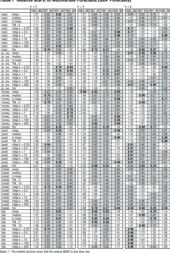
This paper examines the effectiveness of forecasting methods using multiple information variables in forecasting the rate of changes in the consumer price index (CPI) and real GDP in Japan, and investigates the background of forecast performance improvement and its limitations. We first examine the performance of forecasts that use individual information variables as well as forecasts that use multiple information variables. The results show that no single variable improves forecasts in all periods for either CPI or GDP, but combining the information from individual forecasts can lead to a stable forecast performance. Next, to explore the backdrop to these improvements in forecast performance, we decompose and analyze the forecast error of forecast combinations using a simple mean. We discover that the irregular movements of forecast errors generally cancel each other out, which in turn leads to a reduction in errors. At the same time, the effect of reducing forecast errors rapidly diminishes with the addition of variables, and we verify that forecast performance stops improving after two to four variables are added. For this reason, it is necessary to consider both the performance of original forecast series that comprise the combination, and the combination of variables that best reduces the correlation among forecast error series to obtain the optimal combination of series.
Keywords: Information variable; Multivariate forecast; Out-of-sample forecast; Forecast combination
I. Introduction
In recent years, both inside and outside of Japan, much attention has been given to multivariate forecasting methods for inflation and output growth. In this paper, we first evaluate the effectiveness of these methods in Japanese data, and then attempt to highlight mechanisms that improve forecasting performance and also consider the limitations of these mechanisms.
In formulating monetary policy, it is crucial to grasp the current state of the economy and provide an economic outlook. For this purpose, it is necessary to forecast inflation and output growth rates for a certain period ahead, for example, six months, one year, and two years. Thus, there has been a variety of research conducted on such economic forecasting.1
One typical method of forecasting is to use an individual indicator as an information variable based on economic theory.2 For example, real economic variables such as the unemployment rate are likely to contain some information on future inflation, as the Phillips curve can be derived under assumptions such as rigid nominal prices. Another example is that asset prices such as share prices can be considered to contain some information on the future course of the economy, because an asset price is theoretically equal to the present discounted value of future income generated by that asset.3 For this reason, much research has been conducted from the viewpoint of whether useful information for forecasting can be extracted from each individual variable such as money balance, long-term interest rates, share prices, commodity prices, and the unemployment rate.4
However, as a comprehensive survey undertaken by Stock and Watson (2001) shows, a variable with satisfactory effectiveness in forecasting across periods and countries is yet to be found. More specifically, there are virtually no cases in which the theoretical relationship between variables is sufficiently stable in forecasting.5
Based on these results, in recent years there have been many attempts to obtain more accurate forecasts by integrating information from a variety of variables, without relying on a particular information variable that, in theory, appears to contain useful information.
1. This paper focuses on forecasting of future inflation rates and real GDP growth rates (i.e., pinpoint forecasting). On the other hand, forecasting of “turning points” in price movements or the economy is also an important theme in economic forecasting. Recent examples of research that emphasizes forecasting of turning points include Honda and Matsuoka (2001) and Kasuya and Shinki (2001).
2. In this paper, the term “information variable” is defined as a “financial or economic indicator with correlation to and precedence over the final target.” See Kato (1991) for this definition.
3. Okina and Shiratsuka (2002) discuss this point in relation with the monetary policy management based upon the experiences of the bubble period in the 1980s.
4. Other than those mentioned here, variables that have been investigated for their predictive content for inflation and real output include yield spread (i.e., the difference between long- and short-term interest rates), default spread (i.e., the difference between CP and government bond rates), and the exchange rate. Stock and Watson (2001) survey this large literature on various variables including these. As for recent research in Japan focusing on individual variables, Hirata and Ueda (1998) examine the predictive content of yield spread for the economic activity, and both Mio (2001) and Fukuda and Keida (2001) investigate the forecast performance of the Phillips curve for inflation.
5. These results are obtained through more direct empirical analyses in Stock and Watson (1996), Cecchetti et al. (2000), and Stock and Watson (2001).
Among the many kinds of multivariate forecasting methods, two basic approaches have gained attention in recent years. The difference between the two lies in whether combining information comes first and then forecasting, or the reverse order. The former is an “index approach,” where a small number of indices are first constructed from many information variables, and the resulting indices are used for forecasting. The latter is a “forecast combination approach,” where some forecasts are made using individual variables separately at first, and then these forecasts are combined by some means to create a final forecast.6
Stock and Watson (1998) adopt the index approach, and they estimate a dynamic factor model for 170 time-series data in the United States.7 They confirm that the forecast performance of the models to forecast inflation and real industrial produc-tion was better than the forecast performance of the autoregressive (AR) model or other models using individual variables such as the unemployment rate. Similar studies using the index approach are Marcellino et al.(2000) and Forniet al.(2002) for Europe, and Artiset al. (2002) for the United Kingdom. All of these reported high forecast performance for the dynamic factor model.
On the other hand, an example of research that adopts the forecast combination approach is Stock and Watson (2001).8They first construct forecasts for production growth and inflation using 38 economic indicators as individual information variables for seven Organisation for Economic Co-operation and Development (OECD) countries. They then make combination forecasts by taking the median, mean, and trimmed mean of different individual forecasts, and finally evaluate the forecast performance. As a result, they report that the combination forecasts always outperformed forecasts using individual variables, even if the performance of individual forecasts to be combined is unstable.9
Stock and Watson (1999) examine both of these approaches. In their paper, they adopt principal component analysis10as the method of constructing “indexes” for the index approach. The approach taken for forecast combination uses the simple mean,
6. In addition to these, there are approaches where macroeconometric models are used, or many explanatory variables are included directly in forecast models such as vector autoregression (VAR) or state space models. Some examples of recent studies undertaken in Japan that use these approaches include Ban and Saito (2001) for the former and Kitagawa and Kawasaki (2001) for the latter. Also, the successive approximation method, which is widely used in practical economic forecasting, can be seen as an approach that includes as much information as possible into forecasts. Under the successive approximation method, a forecaster responsible for each aspect of the economy such as production or consumption establishes an outlook for that aspect, and each outlook is repeatedly adjusted to make it consistent with the whole. This method could be considered the antithesis of statistical methods.
7. The dynamic factor model assumes that common factors exist behind multiple individual series and it is these factors that dynamically affect individual series. See Stock and Watson (1998) for details.
8. In the field of forecasting theory, this approach has been examined for long time. One of the earliest seminal papers is Bates and Granger (1969).
9. Another recent example of studies that adopts the approach of combining forecast is Marcellino (2002). Also, in Japan, Oyama (2001) calculates a total of five real GDP forecast series, one of which is forecasted using the accumulation format, and the other of which were forecasted using each of four series such as the index of total industry activity as an information variable individually. A forecast combination series was created based on these five series, and it was reported to show high forecast performance.
10. Stock and Watson (1998) show that when there are a large number of variables, under certain technical assumptions the principal component extracted in principal component analysis is a consistent estimator for the factor in the dynamic factor model. This is the backdrop to the fact that they used principal component analysis in Stock and Watson (1999). The adoption of principal component analysis in Section III of this paper is also based on this fact.
the median, and weighted averages whose weights are calculated based on ridge regression.11According to their results, both of these approaches outperform forecast models using individual variables, and in particular the forecast performance using the first principal component extracted by principal component analysis is shown to be superior.
While all of the preceding studies listed above provide evidence supporting the effectiveness of the index or the forecast combination approach, important issues remain unresolved: why do these forecasting methods work better? How many variables should we use in these two methods? In fact, forecasting performance does not simply improve as the number of variables included increases; it has been found that results can actually deteriorate if the number of variables is too large (see Stock and Watson [2001]).12 It is therefore necessary to show both the mechanism that improves forecasting performance in these methods and its limitations, and to investigate the optimal number of variables to be included.
In this paper, we evaluate the effectiveness of these multivariate forecasting methods using Japanese data, based on the framework presented in Stock and Watson (1999), and examine both the mechanism of performance enhancement and the limitation of that mechanism. Our results confirm that these forecasting methods are also effective for Japanese data. We also discover that the improvement and stabilization of performance are primarily created by a canceling out of the irregular movements of forecast errors. At the same time, forecast performance stops improving after the inclusion of two to four variables due to the addition of poorly performing forecast series, because the effect of reducing forecast errors rapidly decreases with the addition of variables.
The remainder of this paper is organized as follows. In Section II, we construct bivariate forecasts for the rate of change in Japan’s CPI and real GDP, by using a variety of financial and economic indicators as information variables within the framework of Stock and Watson (2001). We then review the performance of these bivariate forecasts compared with the forecasting performance based on the AR model. In Section III, we create multivariate forecasts and observe their performance. In Section IV, we consider the mechanisms involved in forecast performance improvements and their limitations. We conclude the paper in Section V.
II. Bivariate Forecasting and Its Results
As preparation for examining the performance improvement mechanism of combined forecasts and its limitations, we first construct bivariate forecasts using various individual information variables based on the framework of Stock and Watson (2001). Specifically, we construct half-year (two-quarter), one-year (four-quarter), and two-year (eight-quarter) ahead forecasts for the rate of changes in CPI and real GDP.
11. See Section III for a forecasting method using ridge regression.
12. According to Watson (2000), the marginal improvement in forecast performance achieved by the addition of information variables in terms of the coefficient of determination rapidly decreases with the increase of the total number of information variables.
A. Forecasting Model
The model here predicts the change in the variable being forecast (Y) up tohperiods in the future, using the current and past information of both the variable being forecast and an information variable (X), or the current and lagged value of these two variables at the time of the forecast.13
yh
t+h= α+ β(L)yt+ γ(L)Xt+ εht+h, (1)
where yt = ln(Yt) – ln(Yt–1) is the logarithmic first difference of Yt, i.e., the rate of changes in CPI or real GDP from a quarter earlier; yh
t+h= ln(Yt+h) – ln(Yt) is the rate of changes in CPI or real GDP from h-quarter earlier; Xt is a candidate leading indicator; αis a constant; and β(L) and γ(L) are the lag polynomials for ytand Xt.
The performance of the bivariate forecast model is evaluated using a comparison with an AR forecast imposing the restriction of γ(L) = 0 in equation (1). That is, the bivariate model above produces an out-of-sample forecast and its mean squared fore-cast error (MSFE), as does the AR model. Then we compare forefore-cast performance using the relative mean squared forecast error (MSFEbivariate forecast/MSFEAR forecast), where the MSFE of the bivariate model is standardized by the MSFE of the corresponding AR model.14 Therefore, the forecast performance of the AR model can be improved by adding information variables if the relative MSFE is below one, meaning an increase in performance.
It should be noted that the addition of information variables does not necessarily improve the out-of-sample forecast performance of a forecast model, while it does improve the in-sample forecast performance.15
B. Data
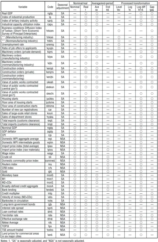
A total of 56 quarterly variables starting in 1970–73 and ending in the first half of 2001 were used as information variable candidates (Table 1).16 We classified these variables into four groups. These are variables regarding real economic activities (index of industrial production, unemployment,Tankan Diffusion Index [DI], etc.),
13. For equation (1), we select an order of lag by Akaike’s information criterion (AIC) in performing a rolling estimation with the sample being the past 40 quarters. Stock and Watson (2001) fix the starting point of the sample and conduct recursive estimation that uses all subsequent data, but we suspect that this recursive estimation is more subject to the effects of changes in economic structure and in the information contained by variables, as the sample length increases. In fact, when we performed recursive estimation on the AR model used as a benchmark below, the forecast performance generally worsened from that of rolling estimation. We adopt AIC rather than Bayesian information criterion (BIC) for a similar reason: when BIC was used to select the order of lag, the forecast performance of the AR model generally worsened when compared to AIC.
14. Similar to Stock and Watson (2001), we employ the AR model as a benchmark. However, the limitations of AR models that rely on only information from past explained variables must be noted.
15. When the sample period used for estimation in a forecast model is from period 0 to period t, “in-sample forecast” indicates the forecast values between period 0 and period t. In contrast, the “out-of-sample forecast,” dealt with in this paper, refers to the forecast values for t+ 1 and later. Out-of-sample forecast is a forecast calculated with only the information available at the time of the forecast, and is more appropriate for the evaluation of the relative merits of forecast models. It should also be noted that although all of the data used in this paper are final revisions, this kind of data is usually unavailable at the time of forecast. For this reason, a precise description of the out-of-sample forecasting in this paper should be “simulated out-of-sample forecasting.”
16. We use final revisions of data in the following analysis. Bernanke and Boivin (2001) apply the method in Stock and Watson (2001) both to real-time data and to data sets consisting of only final revisions, showing that there was no significant difference in the forecast performance of the two.
Table 1 Variables Used in Testing Forecast Ability
Seasonal Nominal/real Average/end-period Processed transformation Variable Code adjustment Nominal Real Ave End Level Log Log diff Gap
— r av ed lev ln ln1d gap
Real GDP rgdp SA — — — —
Index of industrial production ip SA — — — —
Index of tertiary industry activity sanji SA — — — —
Industrial capacity utilization index capu SA — — — —
Business conditions Diffusion Index
of Tankan(Short-Term Economic tnkzen SA — — — —
Survey of Principal Enterprises)
** (Manufacturing industry) tnksei SA — — — —
** (Nonmanufacturing industry) tnkhi SA — — — —
Unemployment rate unemp SA — — — —
Ratio of job offers to applicants kyujin SA — — — —
Machinery orders (private demand) kijmi SA — — — —
Machinery orders kijse SA — — — —
(manufacturing industry)
Machinery orders kijhi SA — — — —
(nonmanufacturing industry)
Construction orders kenjal SA — — — —
Construction orders (private) kenjmi SA — — — —
Construction orders kenjhi SA — — — —
(nonmanufacturing)
Value of public works contracted ukeall SA — — — —
Value of public works contracted ukekun SA — — — —
(central gov’t)
Value of public works contracted ukechi SA — — — —
(local gov’t)
Housing starts juckko SA — — — —
Floor area of housing starts juckme SA — — — —
Floor area of construction starts ckhime SA — — — —
Number of new car registrations car SA — — — —
Sales of large-scale retail stores kouri SA — — — —
Sales of department stores hyaka SA — — — —
Total exports (customs clearance) expt SA — — — —
Total imports (customs clearance) impt SA — — — —
Nominal GDP ngdp SA — — — — —
GDP deflator pgdp SA — — — — —
CPI cpi SA — — — — —
Domestic WPI aggregate average wpi NSA — — — — —
Domestic WPI intermediate goods wpiin NSA — — — —
Import price index (total average) ipiav NSA — — — — —
Import price index (raw materials) ipiso NSA — — — —
Wage index wage SA — — — —
Crude oil oil NSA — — — —
Domestic commodity price index commed NSA — — — —
Reuters index reu NSA — — — —
CRB index crb NSA — — — —
Gold gld NSA — — — —
Monetary base mon0 SA — — — —
M1 mon1 SA — — — —
M2+CDs mon2 SA — — — —
Broadly-defined credit aggregate mon4 SA — — — —
Bank lending lended SA — — — —
Credit multiplier mlp SA — — — —
Velocity of money (M2+CDs) velo SA — — — —
Banknotes in circulation note SA — — —
Long-term government bonds jgb NSA — — —
Interest rate spread sprd NSA — — — — —
Loan contract rates alnd NSA — — — —
Yen/dollar rate rate NSA — —
Effective exchange rate efrat NSA — —
Nikkei Average nik NSA — — —
TOPIX tpx NSA — — —
TSE amount traded tosho NSA — — — —
Land prices for commercial areas land NSA — — — —
in six major cities
Notes: 1. “SA” is seasonally adjusted, and “NSA” is not seasonally adjusted.
2. “Level,” “log,” “log diff,” and “gap” are the processed values of the original values, the logarithmic values, logarithmic difference, and HP filter.
price/wage/market price-related variables (wholesale prices, Commodity Research Bureau [CRB] index, etc.), money-related variables (monetary base, M2+CDs, etc.) and asset price variables (foreign exchange rates, interest rates, share prices, land prices, etc.). Most of these data series are then transformed as follows. First, for series that showed significant seasonal variation, we use seasonally adjusted series where data are officially available, and we create a seasonally adjusted series using X-12-ARIMA where it is not.17Second, when converting monthly data and daily data to quarterly data, we use the end-of-quarter value or the average for the quarter according to the characteristics of each variable. (However we use both the end-of-quarter value and the average for some series, where it cannot be determined which conversion is better.) Third, in some cases, we used not only the original series but also the series transformed by logarithm, logarithmic difference, or HP filter (λ= 1,600).
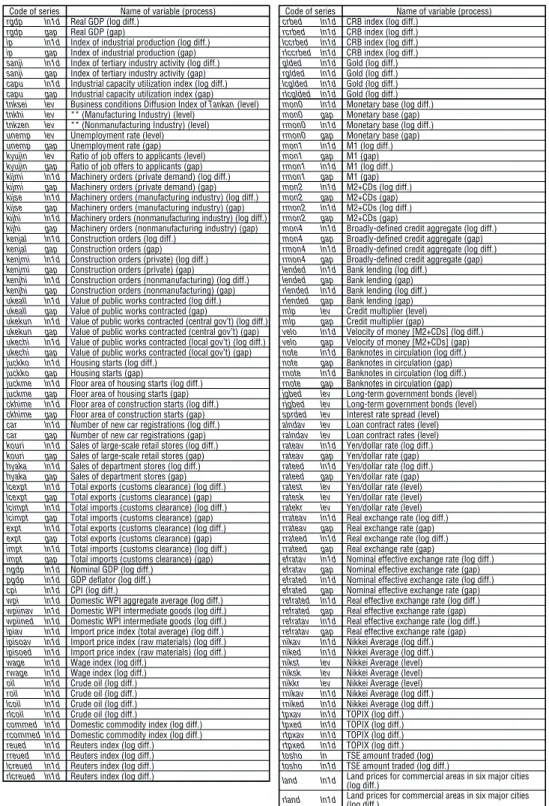
As a result of these transformations, 148 series are used for forecasting the CPI rate of change and 147 for forecasting the real GDP rate of change (Table 2).
C. Forecast Results
In this subsection, we examine the forecast performance of the bivariate model presented in the Section II.A in relation to the benchmark AR model for the rate of change in CPI and real GDP. Here we divide the entire sample period from the first quarter of 1983 to the second quarter of 1999, where out-of-sample forecasting and its evaluation are feasible, into four sub-sample periods: the pre-bubble period (1983–86), the bubble formation period (1987–90), the bubble collapse period (1991–94), and the post-bubble period (1995–99/II). We then observe the differences between the forecast performance in these four periods.
1. CPI forecast
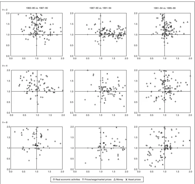
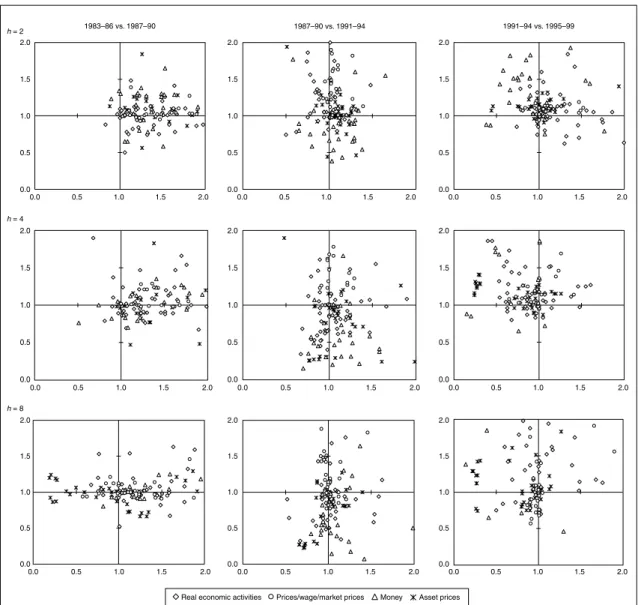
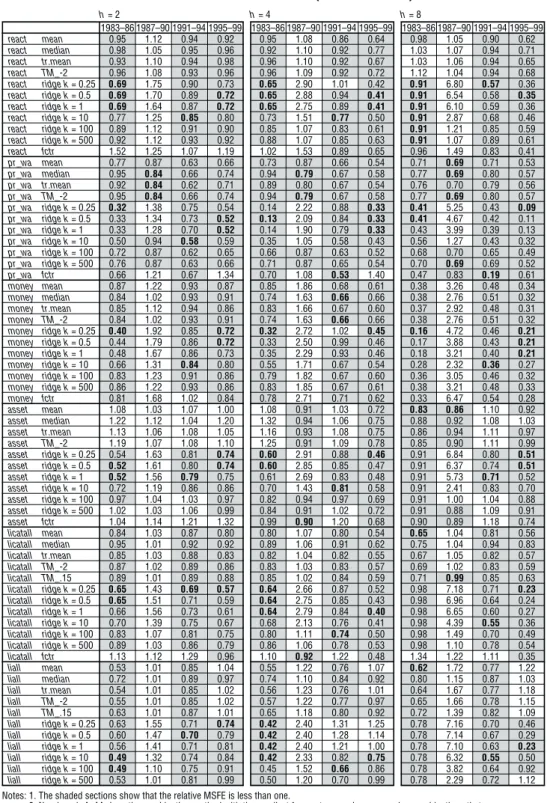
First, we plot the relative MSFE of the bivariate model in two subsequent samples into scatter graphs by forecast horizon, to compare the performance of CPI inflation forecast by sample period and by forecast horizon (Figure 1). The figure shows that the right column of panels has the highest density in the third quadrant, suggesting that the number of series with improved performance increased in the bubble collapse period and the post-bubble period. A closer look at the forecast performance of each information variable offers the observation that the forecast improvement effect of price/wage/market price-related variables is relatively high (Table 3).18,19 However, unfortunately no variable is found that improves forecast performance across all forecast horizons and all sample periods.20
17. For variables that are directly affected by consumption tax (nominal/real GDP, GDP deflator, CPI, new car registrations, sales of large-scale retail stores, sales of department stores), the effect of consumption tax was removed using the X-12-ARIMA seasonal adjustment option. On the other hand, not only the effect of consumption tax but also summer power prices are excluded from domestic wholesale prices.
18. Hereafter we define italic word(s)in parentheses as the abbreviating code(s) of variable, transformation, or both. See Tables 1 and 2 for the codes corresponding to each variable.
19. Looking at the individual sample periods, it appears that some bivariate forecasts including the nominal GDP (ngdp) and wage (wage) in prices/wage, etc., outperformed the AR forecasts. Moreover, M2+CDs (mon2) and real bank lending (rlended) are effective in all periods after the collapse of the bubble. However, performance deteriorates for all of these if the sample period or number of forecast periods is changed.
20. On average, nominal GDP minimizes the relative MSFE across all forecast horizons and sample periods, but even in this case the MSFE exceeds one in the two-quarter-ahead forecast for 1995–99 and eight-quarter-ahead forecast for 1987–90, with forecast performance worse than the AR model.
Code of series Name of variable (process)
rgdp ln1d Real GDP (log diff.)
rgdp gap Real GDP (gap)
ip ln1d Index of industrial production (log diff.)
ip gap Index of industrial production (gap)
sanji ln1d Index of tertiary industry activity (log diff.)
sanji gap Index of tertiary industry activity (gap)
capu ln1d Industrial capacity utilization index (log diff.)
capu gap Industrial capacity utilization index (gap)
tnksei lev Business conditions Diffusion Index of Tankan(level)
tnkhi lev ** (Manufacturing Industry) (level)
tnkzen lev ** (Nonmanufacturing Industry) (level)
unemp lev Unemployment rate (level)
unemp gap Unemployment rate (gap)
kyujin lev Ratio of job offers to applicants (level)
kyujin gap Ratio of job offers to applicants (gap)
kijmi ln1d Machinery orders (private demand) (log diff.)
kijmi gap Machinery orders (private demand) (gap)
kijse ln1d Machinery orders (manufacturing industry) (log diff.)
kijse gap Machinery orders (manufacturing industry) (gap)
kijhi ln1d Machinery orders (nonmanufacturing industry) (log diff.)
kijhi gap Machinery orders (nonmanufacturing industry) (gap)
kenjal ln1d Construction orders (log diff.)
kenjal gap Construction orders (gap)
kenjmi ln1d Construction orders (private) (log diff.)
kenjmi gap Construction orders (private) (gap)
kenjhi ln1d Construction orders (nonmanufacturing) (log diff.)
kenjhi gap Construction orders (nonmanufacturing) (gap)
ukeall ln1d Value of public works contracted (log diff.)
ukeall gap Value of public works contracted (gap)
ukekun ln1d Value of public works contracted (central gov’t) (log diff.)
ukekun gap Value of public works contracted (central gov’t) (gap)
ukechi ln1d Value of public works contracted (local gov’t) (log diff.)
ukechi gap Value of public works contracted (local gov’t) (gap)
juckko ln1d Housing starts (log diff.)
juckko gap Housing starts (gap)
juckme ln1d Floor area of housing starts (log diff.)
juckme gap Floor area of housing starts (gap)
ckhime ln1d Floor area of construction starts (log diff.)
ckhime gap Floor area of construction starts (gap)
car ln1d Number of new car registrations (log diff.)
car gap Number of new car registrations (gap)
kouri ln1d Sales of large-scale retail stores (log diff.)
kouri gap Sales of large-scale retail stores (gap)
hyaka ln1d Sales of department stores (log diff.)
hyaka gap Sales of department stores (gap)
lcexpt ln1d Total exports (customs clearance) (log diff.)
lcexpt gap Total exports (customs clearance) (gap)
lcimpt ln1d Total imports (customs clearance) (log diff.)
lcimpt gap Total imports (customs clearance) (gap)
expt ln1d Total exports (customs clearance) (log diff.)
expt gap Total exports (customs clearance) (gap)
impt ln1d Total imports (customs clearance) (log diff.)
impt gap Total imports (customs clearance) (gap)
ngdp ln1d Nominal GDP (log diff.)
pgdp ln1d GDP deflator (log diff.)
cpi ln1d CPI (log diff.)
wpi ln1d Domestic WPI aggregate average (log diff.)
wpiinav ln1d Domestic WPI intermediate goods (log diff.)
wpiined ln1d Domestic WPI intermediate goods (log diff.)
ipiav ln1d Import price index (total average) (log diff.)
ipisoav ln1d Import price index (raw materials) (log diff.)
ipisoed ln1d Import price index (raw materials) (log diff.)
wage ln1d Wage index (log diff.)
rwage ln1d Wage index (log diff.)
oil ln1d Crude oil (log diff.)
roil ln1d Crude oil (log diff.)
lcoil ln1d Crude oil (log diff.)
rlcoil ln1d Crude oil (log diff.)
commed ln1d Domestic commodity index (log diff.)
rcommed ln1d Domestic commodity index (log diff.)
reued ln1d Reuters index (log diff.)
rreued ln1d Reuters index (log diff.)
lcreued ln1d Reuters index (log diff.)
rlcreued ln1d Reuters index (log diff.)
Table 2 Codes, Variables, and Conversion Methods Used in Each Series
Code of series Name of variable (process)
crbed ln1d CRB index (log diff.)
rcrbed ln1d CRB index (log diff.)
lccrbed ln1d CRB index (log diff.)
rlccrbed ln1d CRB index (log diff.)
glded ln1d Gold (log diff.)
rglded ln1d Gold (log diff.)
lcglded ln1d Gold (log diff.)
rlcglded ln1d Gold (log diff.)
mon0 ln1d Monetary base (log diff.)
mon0 gap Monetary base (gap)
rmon0 ln1d Monetary base (log diff.)
rmon0 gap Monetary base (gap)
mon1 ln1d M1 (log diff.)
mon1 gap M1 (gap)
rmon1 ln1d M1 (log diff.)
rmon1 gap M1 (gap)
mon2 ln1d M2+CDs (log diff.)
mon2 gap M2+CDs (gap)
rmon2 ln1d M2+CDs (log diff.)
rmon2 gap M2+CDs (gap)
mon4 ln1d Broadly-defined credit aggregate (log diff.)
mon4 gap Broadly-defined credit aggregate (gap)
rmon4 ln1d Broadly-defined credit aggregate (log diff.)
rmon4 gap Broadly-defined credit aggregate (gap)
lended ln1d Bank lending (log diff.)
lended gap Bank lending (gap)
rlended ln1d Bank lending (log diff.)
rlended gap Bank lending (gap)
mlp lev Credit multiplier (level)
mlp gap Credit multiplier (gap)
velo ln1d Velocity of money [M2+CDs] (log diff.)
velo gap Velocity of money [M2+CDs] (gap)
note ln1d Banknotes in circulation (log diff.)
note gap Banknotes in circulation (gap)
rnote ln1d Banknotes in circulation (log diff.)
rnote gap Banknotes in circulation (gap)
jgbed lev Long-term government bonds (level)
rjgbed lev Long-term government bonds (level)
sprded lev Interest rate spread (level)
alndav lev Loan contract rates (level)
ralndav lev Loan contract rates (level)
rateav ln1d Yen/dollar rate (log diff.)
rateav gap Yen/dollar rate (gap)
rateed ln1d Yen/dollar rate (log diff.)
rateed gap Yen/dollar rate (gap)
ratest lev Yen/dollar rate (level)
ratesk lev Yen/dollar rate (level)
ratekr lev Yen/dollar rate (level)
rrateav ln1d Real exchange rate (log diff.)
rrateav gap Real exchange rate (gap)
rrateed ln1d Real exchange rate (log diff.)
rrateed gap Real exchange rate (gap)
efratav ln1d Nominal effective exchange rate (log diff.)
efratav gap Nominal effective exchange rate (gap)
efrated ln1d Nominal effective exchange rate (log diff.)
efrated gap Nominal effective exchange rate (gap)
refrated ln1d Real effective exchange rate (log diff.)
refrated gap Real effective exchange rate (gap)
refratav ln1d Real effective exchange rate (log diff.)
refratav gap Real effective exchange rate (gap)
nikav ln1d Nikkei Average (log diff.)
niked ln1d Nikkei Average (log diff.)
nikst lev Nikkei Average (level)
niksk lev Nikkei Average (level)
nikkr lev Nikkei Average (level)
rnikav ln1d Nikkei Average (log diff.)
rniked ln1d Nikkei Average (log diff.)
tpxav ln1d TOPIX (log diff.)
tpxed ln1d TOPIX (log diff.)
rtpxav ln1d TOPIX (log diff.)
rtpxed ln1d TOPIX (log diff.)
tosho ln TSE amount traded (log)
tosho ln1d TSE amount traded (log diff.)
land ln1d Land prices for commercial areas in six major cities
(log diff.)
rland ln1d Land prices for commercial areas in six major cities (log diff.)
Note: The start of the data is 1970, except the following series: 1973 for the index of tertiary industry activity, 1971 for construction orders (kenjal, kenjmi, kenjhi), 1973 for the value of public works contracted (ukeall, ukekun, ukechi), 1971 for long-term government bonds (jgbed, rjgbed), 1973 for the yen/dollar rate and related indicators (rateav, rateed, ratest, ratesk, ratekr, rrateav, rrated, efratav, efrated, refrated, refratav), and 1972 for some of the Nikkei Average (nikst, niksk, nikkr).
Figure 1 Performance of CPI Forecasts 2.0 1.5 1.0 0.5 0.0 2.0 1.5 1.0 0.5 0.0 2.0 1.5 1.0 0.5 0.0 0.0 0.5 1.0 1.5 2.0 2.0 1.5 1.0 0.5 0.0 0.0 0.5 1.0 1.5 2.0 2.0 1.5 1.0 0.5 0.0 0.0 0.5 1.0 1.5 2.0 0.0 0.5 1.0 1.5 2.0 2.0 1.5 1.0 0.5 0.0 0.0 0.5 1.0 1.5 2.0 2.0 1.5 1.0 0.5 0.0 0.0 0.5 1.0 1.5 2.0 0.0 0.5 1.0 1.5 2.0 2.0 1.5 1.0 0.5 0.0 0.0 0.5 1.0 1.5 2.0 2.0 1.5 1.0 0.5 0.0 0.0 0.5 1.0 1.5 2.0 h = 2 h = 4 h = 8 1983–86 vs. 1987–90 1987–90 vs. 1991–94 1991–94 vs. 1995–99
Real economic activities Prices/wage/market prices Money Asset prices
Note: Each group of graphs (horizontal axis and vertical axis) shows the relative MSFE for (1983–86, 1987–90), (1987–90, 1991–94), and (1991–94, 1995–99/II). If the relative MSFE is one or less, the performance is an improvement on the AR model, meaning that the information variables in the third quadrant of each graph show improved performance over the AR model for two consec-utive sample periods. Additionally, a comparison of the graphs along the horizontal direction confirms how forecast performance changes between sample periods while the forecast horizon, hin equation (1), is constant. Also a comparison of the graphs along the vertical direction confirms how forecast performance changes between forecast horizons while the sample period is kept constant.
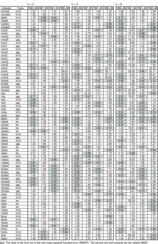
Table 3 Performance of CPI Forecasts h= 2 h= 4 h= 8 Indicator Trans. 1983–86 1987–90 1991–94 1995–99 1983–86 1987–90 1991–94 1995–99 1983–86 1987–90 1991–94 1995–99 AR RMSFE 1.38 0.91 0.72 0.55 1.66 0.76 0.69 0.59 2.98 0.62 0.88 0.77 rgdp ln1d 2.03 1.63 0.68 1.36 2.02 2.56 0.48 0.79 0.55 4.10 0.52 0.29 rgdp gap 0.91 1.31 0.92 1.74 1.15 1.78 0.63 1.23 0.59 2.57 0.42 1.00 ip ln1d 0.73 1.77 1.07 1.60 0.58 2.27 0.92 1.38 0.71 2.50 0.89 0.93 ip gap 0.58 1.36 0.98 2.11 0.59 1.52 0.77 2.38 0.69 2.48 0.84 2.03 sanji ln1d 1.49 2.51 0.92 0.97 1.12 12.71 0.93 0.95 2.58 97.55 0.99 0.92 sanji gap 1.61 1.77 0.95 1.04 1.52 4.73 1.07 1.12 2.68 29.89 1.28 1.00 capu ln1d 0.80 1.79 1.01 1.10 0.71 2.22 1.04 1.51 0.87 2.57 1.04 1.33 capu gap 0.93 1.18 1.00 2.38 1.12 1.29 0.96 2.42 1.44 1.86 0.90 2.05 tnksei lev 1.08 1.69 0.81 2.01 1.10 2.93 0.31 1.37 0.94 5.33 0.38 0.83 tnkhi lev 0.70 1.00 0.72 1.06 0.59 1.91 0.30 0.71 0.82 20.39 0.24 0.42 tnkzen lev 0.94 2.03 0.85 2.12 0.95 3.52 0.34 1.24 0.89 8.12 0.41 0.65 unemp lev 4.16 1.38 1.25 3.59 4.49 2.14 1.41 4.70 1.12 3.01 2.40 1.62 unemp gap 1.11 1.68 0.87 2.71 1.40 2.15 0.45 2.89 1.72 1.31 0.45 1.63 kyujin lev 0.54 8.09 1.12 0.60 0.44 28.76 0.82 0.18 0.51 92.43 0.68 0.41 kyujin gap 0.75 3.33 0.99 3.14 0.39 4.97 0.46 3.38 0.36 6.44 0.31 2.50 kijmi ln1d 1.06 1.23 1.01 1.56 1.07 1.44 0.88 1.52 1.08 1.23 0.85 0.83 kijmi gap 0.84 1.61 0.94 2.15 0.99 2.05 0.83 2.55 1.16 1.67 0.70 2.01 kijse ln1d 0.72 1.35 0.97 1.32 0.89 1.30 0.87 1.94 0.95 2.38 0.87 1.11 kijse gap 0.76 2.03 0.91 1.64 0.78 2.58 0.93 2.38 1.01 2.81 0.66 2.20 kijhi ln1d 1.95 1.14 0.92 1.35 1.60 1.13 1.02 0.97 1.37 1.41 0.97 0.72 kijhi gap 1.61 0.99 1.17 2.12 2.60 1.08 1.53 2.35 1.93 1.21 1.55 1.71 kenjal ln1d 1.09 1.01 1.01 1.04 0.97 1.09 0.92 0.63 1.27 1.03 0.91 0.43 kenjal gap 0.95 1.01 0.95 1.06 0.94 1.07 0.78 1.04 1.44 1.08 0.79 1.14 kenjmi ln1d 0.78 1.95 1.04 1.14 0.90 1.33 0.98 0.57 1.18 0.89 0.88 0.55 kenjmi gap 0.88 1.25 1.22 1.16 0.73 1.42 1.09 1.26 1.07 0.99 1.06 1.48 kenjhi ln1d 0.87 1.54 1.09 1.16 0.78 1.37 0.88 0.78 1.15 1.20 0.92 0.56 kenjhi gap 0.80 1.82 1.09 1.21 0.64 1.28 1.58 1.26 0.95 0.99 1.73 1.32 ukeall ln1d 1.00 1.14 1.28 1.04 1.00 1.11 1.21 1.17 0.99 1.87 1.06 1.00 ukeall gap 1.23 1.16 1.32 1.21 0.96 1.70 1.33 1.91 2.07 6.75 1.10 1.02 ukekun ln1d 1.02 1.08 1.29 1.01 1.00 1.11 1.18 1.01 1.00 1.13 1.07 0.99 ukekun gap 1.29 1.08 1.58 1.15 1.67 1.08 1.63 1.41 3.00 6.16 1.23 1.20 ukechi ln1d 0.96 1.15 1.04 1.04 0.99 1.06 1.06 1.12 1.01 1.79 1.01 1.01 ukechi gap 1.10 1.16 1.08 1.23 0.83 1.87 1.18 1.50 1.54 5.94 1.03 0.94 juckko ln1d 1.24 0.97 1.11 1.41 1.08 1.06 1.06 1.76 0.68 1.39 1.21 2.32 juckko gap 1.34 0.65 1.26 2.24 1.21 0.72 1.75 2.90 1.06 0.95 1.93 3.53 juckme ln1d 1.54 0.96 0.94 1.69 1.27 1.12 0.81 2.00 0.49 1.85 0.93 2.60 juckme gap 1.33 0.55 1.26 2.90 1.14 0.73 1.81 3.63 0.85 1.54 1.31 4.63 ckhime ln1d 1.17 1.16 1.07 1.33 1.03 1.21 1.40 1.12 0.64 0.82 0.54 0.92 ckhime gap 0.74 0.99 1.02 1.47 0.61 0.91 0.77 2.43 0.72 0.96 0.63 2.21 car ln1d 0.98 1.01 0.99 0.65 1.37 1.18 0.68 0.65 0.80 8.89 0.44 0.74 car gap 0.60 1.88 1.27 1.18 0.41 5.04 1.25 0.91 0.46 13.18 0.76 1.45 kouri ln1d 0.92 1.10 0.87 1.23 0.78 1.09 1.42 0.52 0.47 4.05 0.34 0.45 kouri gap 1.67 2.39 0.95 1.33 1.80 6.92 0.49 0.98 1.78 27.46 0.59 1.76 hyaka ln1d 1.34 1.54 1.09 1.48 1.21 1.55 0.85 1.55 0.53 3.81 0.32 1.11 hyaka gap 1.05 1.66 0.85 1.95 1.35 3.84 0.57 2.35 1.68 9.76 0.38 2.68 lcexpt ln1d 0.67 0.77 1.46 1.62 0.66 1.95 1.27 1.60 0.92 5.16 1.03 2.54 lcexpt gap 0.64 2.11 1.17 3.01 0.69 5.84 1.28 3.46 1.01 15.65 1.06 4.78 lcimpt ln1d 0.95 2.47 1.09 0.95 0.88 2.49 1.43 1.12 1.06 2.58 1.28 2.12 lcimpt gap 0.75 4.09 0.86 2.85 0.86 6.59 1.01 2.86 1.08 15.46 0.93 3.05 expt ln1d 0.88 1.89 0.95 1.75 1.00 0.99 0.98 1.51 1.00 0.97 1.05 1.10 expt gap 0.89 0.88 1.15 2.30 0.74 0.64 1.31 2.34 1.13 0.67 0.98 2.08 impt ln1d 1.10 3.96 0.95 1.38 1.08 7.55 0.97 1.43 0.98 7.90 1.27 0.75 impt gap 1.26 3.20 0.91 1.87 1.33 5.36 0.75 2.07 1.17 11.11 0.98 1.23 ngdp ln1d 0.87 0.93 0.56 1.04 0.94 0.79 0.38 0.73 0.48 1.04 0.43 0.19 pgdp ln1d 1.32 1.12 0.74 1.77 1.35 1.74 0.65 1.61 1.11 0.95 0.89 1.12 wpi ln1d 0.44 2.28 0.82 1.45 0.42 2.58 1.16 1.76 1.03 4.20 0.97 1.53 wpiinav ln1d 0.54 2.01 1.20 1.57 0.40 2.41 1.01 2.04 0.95 3.66 0.99 1.95 wpiined ln1d 0.30 1.94 1.15 1.18 0.26 2.07 1.04 2.02 0.66 2.96 1.02 1.90 ipiav ln1d 0.82 1.45 1.02 1.04 0.89 1.50 1.21 0.97 0.90 1.73 1.27 1.88 ipisoav ln1d 1.30 1.73 1.02 1.03 1.40 2.07 1.20 1.03 0.97 4.85 1.28 1.51 ipisoed ln1d 1.37 1.73 1.08 1.03 1.59 4.41 1.19 0.94 1.04 1.97 1.40 1.28 wage ln1d 1.01 0.80 0.70 1.77 1.03 0.40 0.61 1.85 0.71 0.41 0.29 1.12 rwage ln1d 1.13 0.89 0.67 1.11 1.08 1.49 0.83 1.07 0.67 1.87 0.99 0.97 oil ln1d 1.32 2.64 1.43 1.02 0.90 4.31 1.22 1.01 0.86 3.02 1.04 1.00 roil ln1d 1.39 2.71 1.43 1.02 1.00 4.50 1.23 1.02 0.83 3.17 1.04 1.00 lcoil ln1d 1.16 1.76 1.36 1.12 1.64 2.12 1.26 1.00 0.92 2.20 1.01 1.07 rlcoil ln1d 1.18 1.70 1.36 1.12 1.61 2.06 1.26 1.00 0.91 2.22 1.01 1.07 commed ln1d 0.77 3.74 0.92 1.02 0.79 3.54 1.01 1.11 0.57 2.61 0.72 1.52 rcommed ln1d 0.77 3.69 0.93 1.03 0.80 3.49 1.02 1.14 0.57 2.68 0.77 1.52 reued ln1d 1.64 1.49 0.96 1.21 1.69 2.93 0.98 1.33 0.97 4.52 1.03 1.11 rreued ln1d 1.93 1.32 0.95 1.22 1.97 2.60 0.96 1.42 1.06 3.89 1.02 1.12 lcreued ln1d 0.99 1.97 1.31 0.89 1.24 2.57 1.36 0.87 0.92 1.45 1.44 1.55 rlcreued ln1d 0.98 2.02 1.29 0.89 1.19 2.58 1.35 0.86 0.92 1.65 1.43 1.55 crbed ln1d 1.87 2.19 1.02 1.44 2.35 2.72 1.20 0.96 1.26 2.57 1.21 1.00 rcrbed ln1d 2.48 2.13 1.03 1.20 3.07 2.48 1.29 1.17 1.52 2.44 1.24 1.04
Table 3 (continued) h= 2 h= 4 h= 8 Indicator Trans. 1983–86 1987–90 1991–94 1995–99 1983–86 1987–90 1991–94 1995–99 1983–86 1987–90 1991–94 1995–99 lccrbed ln1d 1.22 1.70 1.41 1.67 1.39 1.70 1.49 1.22 1.06 2.53 1.46 1.89 rlccrbed ln1d 1.26 1.68 1.41 1.69 1.37 1.72 1.50 1.25 1.00 2.75 1.28 1.84 glded ln1d 1.78 0.99 0.94 1.80 1.14 1.58 0.97 1.97 0.74 3.26 1.01 1.94 rglded ln1d 1.81 0.99 0.92 1.78 1.22 1.56 1.01 1.97 0.81 3.14 1.00 2.00 lcglded ln1d 1.52 1.24 1.18 1.05 0.77 1.58 1.16 0.96 0.89 2.31 1.11 0.97 rlcglded ln1d 1.54 1.25 1.20 1.06 0.78 1.52 1.12 0.95 0.89 2.35 1.12 0.99 mon0 ln1d 0.94 3.23 1.00 1.30 1.11 7.47 0.91 1.36 0.63 14.04 0.47 0.68 mon0 gap 3.32 0.94 1.74 1.57 3.45 2.70 1.43 1.54 1.85 15.19 0.68 1.57 rmon0 ln1d 1.06 2.56 0.99 1.40 1.09 6.43 0.92 1.33 0.63 11.91 0.86 0.57 rmon0 gap 1.19 1.65 2.80 1.32 1.19 5.32 3.13 1.31 0.54 10.72 1.79 2.10 mon1 ln1d 0.81 1.05 1.19 1.03 0.84 3.13 1.64 1.03 0.39 8.95 1.13 0.96 mon1 gap 3.66 0.47 1.46 1.14 2.99 0.50 2.00 1.74 1.94 5.44 1.32 2.39 rmon1 ln1d 0.77 1.09 1.21 1.03 0.78 3.74 1.54 1.02 0.40 9.91 1.12 0.96 rmon1 gap 1.08 1.38 1.62 1.37 0.95 9.13 2.03 2.35 0.68 27.32 1.71 2.43 mon2 ln1d 1.12 1.52 1.02 1.09 1.09 3.58 0.77 0.76 0.22 9.55 0.81 0.42 mon2 gap 2.32 1.65 1.26 1.34 2.21 5.41 0.93 1.49 1.23 26.86 0.79 1.77 rmon2 ln1d 1.14 1.17 0.90 0.84 1.01 3.45 0.70 0.71 0.22 7.51 0.75 0.36 rmon2 gap 0.71 2.63 2.33 1.15 0.63 5.31 3.70 1.05 0.09 10.28 4.24 1.50 mon4 ln1d 0.59 0.80 1.50 57.19 0.59 0.92 3.60 54.57 0.16 1.77 2.77 33.32 mon4 gap 2.15 1.52 1.02 58.63 2.03 5.07 0.82 92.11 1.38 28.56 0.96 52.17 rmon4 ln1d 0.74 1.34 1.19 50.90 0.48 1.67 1.67 47.13 0.22 3.42 1.54 33.41 rmon4 gap 0.42 1.26 2.01 43.98 0.42 1.52 2.78 80.89 0.09 2.76 2.68 45.50 lended ln1d 1.54 1.48 1.01 0.92 1.99 1.05 0.67 0.58 0.99 1.68 0.48 0.16 lended gap 2.87 2.11 1.37 1.28 3.48 3.42 1.12 1.50 2.33 5.28 2.65 1.41 rlended ln1d 1.35 1.68 0.97 0.83 1.83 1.19 0.60 0.53 0.87 1.67 0.64 0.13 rlended gap 1.15 2.43 2.76 1.08 0.54 8.20 5.21 1.07 0.17 22.08 7.48 1.03 mlp lev 1.19 4.65 1.75 1.05 1.95 15.43 1.51 1.42 1.14 44.30 2.83 0.84 mlp gap 0.77 1.00 1.89 1.59 0.75 0.67 2.13 1.81 0.52 19.87 0.87 1.71 velo ln1d 0.88 1.05 1.05 1.25 0.70 1.07 1.12 1.68 0.42 1.72 1.09 1.14 velo gap 0.89 1.72 1.29 1.22 1.18 2.98 0.94 1.49 0.43 6.87 0.89 1.73 note ln1d 0.93 1.53 1.17 1.47 1.00 3.96 0.95 1.42 0.57 8.93 0.45 1.04 note gap 2.61 1.29 2.01 1.58 3.71 2.47 1.17 1.76 1.79 16.50 0.50 1.90 rnote ln1d 0.96 1.06 1.00 1.55 0.89 3.75 0.95 1.18 0.53 6.80 0.42 0.79 rnote gap 1.05 1.46 2.55 1.31 1.11 3.72 2.59 1.39 0.64 7.33 2.08 1.83 jgbed lev 0.33 2.27 1.28 0.92 0.36 1.72 1.26 0.64 0.87 9.92 0.93 0.22 rjgbed lev 0.52 1.20 1.08 0.83 0.32 1.32 1.04 0.61 0.81 2.64 0.85 0.64 sprded lev 0.45 1.15 1.26 1.40 0.30 1.26 1.83 1.42 0.43 1.61 1.97 1.35 alndav lev 1.00 2.27 1.14 0.96 1.06 4.06 0.68 0.72 1.30 10.81 0.87 1.72 ralndav lev 0.96 0.95 1.24 1.55 1.15 3.69 1.88 1.31 1.23 8.21 2.21 1.34 rateav ln1d 1.00 1.45 1.06 2.21 0.61 1.13 1.00 2.02 1.22 2.39 1.13 2.11 rateav gap 1.11 1.74 1.02 2.86 1.08 4.38 1.15 3.81 1.96 7.53 1.20 4.37 rateed ln1d 1.17 1.94 1.08 2.24 0.35 1.62 1.10 2.43 0.60 3.04 1.11 2.57 rateed gap 1.20 1.90 1.04 2.76 0.67 2.77 1.13 3.90 1.83 7.19 1.18 4.27 ratest lev 1.31 0.81 1.09 1.53 1.00 0.81 1.02 1.22 0.87 1.14 0.92 1.51 ratesk lev 1.03 1.03 1.00 0.94 0.60 2.93 1.07 0.90 1.33 2.75 1.01 0.98 ratekr lev 2.37 1.01 1.04 1.20 1.36 0.96 1.13 1.12 2.10 0.98 1.21 1.05 rrateav ln1d 1.19 1.34 1.05 2.26 0.82 0.99 0.97 2.16 1.00 2.73 1.06 2.05 rrateav gap 1.01 1.79 0.96 2.93 0.81 3.48 1.03 3.86 1.42 6.54 1.05 4.41 rrateed ln1d 0.97 1.46 1.02 2.41 0.61 0.99 0.97 2.60 0.86 2.57 1.06 2.36 rrateed gap 0.94 1.81 0.95 3.11 0.64 3.01 1.04 4.01 1.48 5.75 1.00 4.41 efratav ln1d 0.94 1.49 0.94 1.94 0.72 1.26 0.99 1.71 0.62 1.92 0.94 2.70 efratav gap 0.82 1.57 0.82 2.34 0.88 2.76 0.53 4.12 1.20 6.62 0.58 5.30 efrated ln1d 1.06 1.67 0.92 1.90 0.70 1.40 1.06 1.95 0.53 2.01 0.98 2.76 efrated gap 0.99 2.07 0.79 2.53 0.80 2.43 0.72 3.12 1.11 5.72 0.60 4.72 refrated ln1d 0.94 1.41 0.99 1.81 0.67 1.17 1.03 1.49 0.53 0.91 1.04 2.46 refrated gap 0.93 1.75 0.85 2.17 0.83 1.84 0.80 3.18 1.41 3.71 0.70 4.09 refratav ln1d 1.15 1.48 0.90 1.64 0.71 1.26 1.12 1.56 0.46 0.95 1.09 2.66 refratav gap 1.02 1.83 0.82 2.23 0.75 1.74 0.92 2.95 1.07 3.67 0.70 4.41 nikav ln1d 1.54 1.11 1.26 1.39 1.67 0.95 1.22 0.70 0.98 1.12 1.23 0.95 niked ln1d 1.07 1.79 1.22 1.36 1.56 1.16 1.21 1.12 1.18 1.50 1.11 1.09 nikst lev 1.01 1.27 1.02 1.23 1.14 13.98 0.99 0.70 1.12 28.38 1.03 0.56 niksk lev 1.01 2.58 1.17 1.15 0.98 2.89 2.55 1.00 1.01 3.74 2.94 0.91 nikkr lev 1.07 1.32 1.05 1.04 0.96 1.25 1.04 1.00 0.95 1.13 1.01 0.92 rnikav ln1d 1.67 1.11 1.25 1.39 1.63 0.95 1.22 0.81 0.94 1.13 1.24 0.95 rniked ln1d 1.03 1.85 1.22 1.36 1.42 1.20 1.21 1.12 1.17 1.54 1.12 1.09 tpxav ln1d 1.18 1.37 1.15 1.32 1.49 1.06 1.15 0.98 1.03 1.10 1.23 1.11 tpxed ln1d 0.82 1.71 0.97 1.36 1.26 1.36 1.15 1.16 1.20 1.56 1.10 1.12 rtpxav ln1d 1.23 1.38 1.15 1.32 1.45 1.06 1.15 0.98 1.05 1.11 1.72 1.12 rtpxed ln1d 0.82 1.77 0.97 1.36 1.29 1.39 1.14 1.17 1.19 1.62 1.10 1.13 tosho ln 1.54 1.03 1.00 0.94 1.05 1.15 0.46 1.38 0.84 3.21 0.35 0.69 tosho ln1d 1.45 0.97 1.08 0.98 1.29 1.04 1.21 1.26 0.97 1.19 1.15 1.33 land ln1d 1.41 0.79 2.11 1.26 2.44 3.27 2.96 1.05 1.19 56.48 2.57 0.54 rland ln1d 1.48 0.75 2.13 1.24 2.17 1.01 3.18 1.02 1.04 61.47 3.38 0.52
Note: The value in the first row is the root mean squared forecast error (RMSFE). The second row and onwards are the relative MSFE. The shaded sections are for a relative MSFE of less than one. Note that the forecast data for 1983–85 are missing for series regarding economic activity levels and asset values that start between 1971 and 1973, so 1983–86 uses a mean that does not include the data for this period.
2. Real GDP forecast
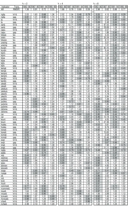
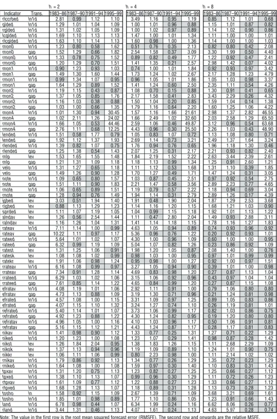
We also calculate the relative MSFE of the bivariate forecast of real GDP growth for each series as we did for CPI. We graph them by forecast horizon and by sample period (Figure 2). Comparing the rows and columns of panels, it appears that the best performance is achieved for one- and two-year forecasts in the bubble formation period, bubble collapse period, and post-bubble period. Moreover, examining the forecast performance of each information variable indicates a high forecast improve-ment effect in money and asset prices (Table 4).21 However, forecast performance does not improve across all forecast horizons and sample periods, which is similar to CPI forecasts in terms of robustness toward differences between samples.22
3. Overview: bivariate forecasting
According to the results in the previous subsections, bivariate forecasts are deemed not to constantly improve the performance of AR forecasts in either the case of CPI forecasts or real GDP forecasts. That is, although performance may be improved in one sample period, it is uncertain that information variables will improve forecast performance in another sample period. The evidence shows that the results of Stock and Watson (2001) are consistent with Japanese time-series data.
III. Multivariate Forecasting and Its Results
In the previous section, we have shown that in a bivariate forecasting framework using individual information variables, forecast performance cannot always be improved for either CPI inflation or real GDP growth across different forecast horizons or sample periods. However, there is a possibility that forecast performance can be improved by appropriately extracting information useful for forecasting from more variables. In this regard, this section first describes multivariate forecasting methods and then compares the performance of the forecasts.
A. Multivariate Forecasting Methods
We now consider forecasting methods used when not only one information variable, but n series (X1, X2, . . . , Xn) are available. There are several variations of actual combination methods, but as we note in Section I, these can be classified into the groups of “index approach” and “forecast combination approach” according to whether the combining of information is conducted before or after the forecast. Following Stock and Watson (1999), this paper adopts principal component analysis for the former and variations of both simple and weighted averages for the latter.
21. With regard to monetary aggregates, in four-quarter- and eight-quarter-ahead forecasts, monetary base
(mon0 ln1d) and M2+CDs (mon2 ln1d) show improvements over longer periods than other variables.
Moreover, with regard to asset prices, forecasts improve over two consecutive sample periods in four-quarter- and eight-quarter-ahead forecasts for nominal exchange rates (rateav ln1d), effective exchange rates (efratav gap), the Nikkei Average (nikav ln1d), TOPIX (tpxav ln1d), etc.
22. The only individual variable that continually improved forecasts from the bubble formation period to the post-bubble period is M2+CDs (mon2 ln1d). However, the relative MSFE for this variable in the 1983–86 period is consistently greater than one, and in four-quarter-ahead forecasts the relative MSFE also exceeded one in the 1987–90 sample period.
Figure 2 Performance of Real GDP Forecasts 2.0 1.5 1.0 0.5 0.0 0.0 0.5 1.0 1.5 2.0 2.0 1.5 1.0 0.5 0.0 0.0 0.5 1.0 1.5 2.0 2.0 1.5 1.0 0.5 0.0 0.0 0.5 1.0 1.5 2.0 2.0 1.5 1.0 0.5 0.0 0.0 0.5 1.0 1.5 2.0 2.0 1.5 1.0 0.5 0.0 0.0 0.5 1.0 1.5 2.0 2.0 1.5 1.0 0.5 0.0 0.0 0.5 1.0 1.5 2.0 2.0 1.5 1.0 0.5 0.0 0.0 0.5 1.0 1.5 2.0 2.0 1.5 1.0 0.5 0.0 0.0 0.5 1.0 1.5 2.0 2.0 1.5 1.0 0.5 0.0 0.0 0.5 1.0 1.5 2.0 h = 2 h = 4 h = 8 1983–86 vs. 1987–90 1987–90 vs. 1991–94 1991–94 vs. 1995–99
Real economic activities Prices/wage/market prices Money Asset prices
Note: Each group of graphs (horizontal axis and vertical axis) shows the relative MSFE for (1983–86, 1987–90), (1987–90, 1991–94), and (1991–94, 1995–99/II). If the relative MSFE is one or less, the performance is an improvement on the AR model, meaning that the information variables in the third quadrant of each graph show improved performance over the AR model for two consec-utive sample periods. Additionally, a comparison of the graphs along the horizontal direction confirms how forecast performance changes between sample periods while the forecast horizon, hin equation (1), is constant. Also a comparison of the graphs along the vertical direction confirms how forecast performance changes between forecast horizons while the sample period is kept constant.
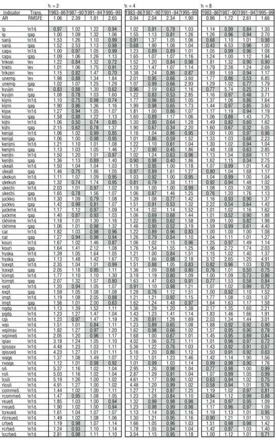
Table 4 Performance of Real GDP Forecasts h= 2 h= 4 h= 8 Indicator Trans. 1983–86 1987–90 1991–94 1995–99 1983–86 1987–90 1991–94 1995–99 1983–86 1987–90 1991–94 1995–99 AR RMSFE 1.06 2.39 1.81 2.65 0.94 2.04 2.34 1.90 0.86 1.72 2.61 1.66 ip ln1d 0.97 1.02 1.22 0.94 1.02 0.91 0.78 1.03 1.14 0.99 0.84 1.30 ip gap 1.00 1.09 1.32 1.06 1.55 1.13 0.81 1.26 1.26 0.96 0.94 2.70 sanji ln1d 1.53 1.26 1.10 0.99 0.91 1.37 1.05 1.06 0.68 1.10 1.01 0.98 sanji gap 1.52 2.53 1.13 0.98 0.68 1.90 1.08 1.04 0.43 6.53 0.96 1.00 capu ln1d 1.00 0.97 1.05 0.99 1.23 0.89 0.89 1.01 1.05 0.99 0.96 1.08 capu gap 1.09 1.06 1.26 1.13 1.65 1.07 1.07 1.16 1.24 1.00 1.12 1.94 tnksei lev 1.22 0.84 1.32 0.72 1.52 1.20 0.84 0.98 1.81 1.32 0.90 0.90 tnkhi lev 1.01 1.06 1.75 0.91 1.22 1.47 1.07 1.14 1.79 2.38 1.24 2.69 tnkzen lev 1.15 0.82 1.47 0.70 1.38 1.24 0.86 0.87 1.89 1.59 0.94 1.17 unemp lev 1.98 0.88 1.34 1.84 2.01 0.95 0.66 3.60 1.77 0.86 0.53 6.85 unemp gap 1.02 1.07 1.25 1.29 1.07 0.99 0.66 2.93 1.29 1.02 0.77 1.79 kyujin lev 0.83 0.88 1.30 0.62 0.96 2.59 0.63 1.16 0.77 5.74 0.25 2.31 kyujin gap 1.08 0.78 1.03 1.60 1.22 0.83 0.53 2.85 1.16 0.97 0.48 3.71 kijmi ln1d 1.10 0.75 0.98 0.74 1.77 0.96 0.65 1.05 1.37 1.06 0.86 1.64 kijmi gap 1.90 0.86 1.36 1.16 1.99 0.98 0.65 1.73 1.44 0.97 0.85 3.60 kijse ln1d 1.27 0.94 1.05 1.07 1.81 1.00 0.86 1.07 1.17 1.19 0.94 1.19 kijse gap 1.58 0.88 1.22 1.13 1.60 0.89 1.17 1.06 1.06 0.88 1.43 1.75 kijhi ln1d 1.06 0.50 0.74 0.85 1.30 0.90 0.64 1.28 1.49 0.82 0.60 1.62 kijhi gap 2.15 0.62 0.78 1.37 1.90 0.67 0.34 2.20 1.60 0.67 0.32 5.05 kenjal ln1d 1.06 1.02 0.99 0.85 1.16 1.04 0.86 0.95 1.00 1.00 0.97 0.96 kenjal gap 1.06 1.00 0.98 0.95 1.01 0.86 0.59 1.52 1.33 1.03 0.68 2.23 kenjmi ln1d 1.21 1.10 1.01 1.08 1.22 1.10 0.61 1.04 1.30 1.02 0.94 1.04 kenjmi gap 1.13 1.03 1.05 1.46 1.27 0.90 0.45 1.86 1.48 1.08 0.63 2.85 kenjhi ln1d 1.50 1.20 1.01 0.97 1.02 1.24 0.63 0.96 1.13 1.54 0.69 1.17 kenjhi gap 1.36 1.13 0.89 1.40 0.90 0.98 0.40 1.86 1.62 1.15 0.34 2.75 ukeall ln1d 1.50 1.04 1.04 1.03 1.15 0.95 1.00 1.18 1.07 0.99 1.01 1.43 ukeall gap 1.46 0.75 1.86 1.05 0.97 0.89 1.61 1.27 0.80 1.04 1.68 1.17 ukekun ln1d 1.11 1.07 1.09 0.95 1.03 0.92 1.00 0.95 1.04 0.99 1.00 1.04 ukekun gap 1.32 0.74 1.74 0.95 0.81 0.79 1.38 1.11 0.92 0.94 1.48 1.02 ukechi ln1d 2.03 1.01 0.97 1.02 1.19 1.00 1.00 0.99 1.08 1.03 1.00 1.35 ukechi gap 1.65 0.78 1.56 1.07 1.06 0.87 1.46 1.25 0.76 1.20 1.76 1.13 juckko ln1d 1.30 1.09 0.79 1.08 1.39 1.08 0.77 1.42 1.16 0.93 0.90 1.37 juckko gap 1.42 0.99 0.81 1.07 1.51 0.91 0.53 1.32 2.22 0.54 0.64 1.42 juckme ln1d 1.17 1.12 0.97 1.09 1.14 1.02 1.14 1.52 1.01 1.02 1.16 1.62 juckme gap 1.40 0.87 0.93 1.03 1.06 0.69 0.68 1.44 1.01 0.52 0.90 1.88 ckhime ln1d 1.18 1.01 1.30 1.16 1.22 0.95 0.62 1.58 1.09 1.00 0.82 1.98 ckhime gap 1.06 1.01 0.98 1.32 1.46 0.90 0.52 3.19 1.59 0.99 0.61 4.40 car ln1d 1.82 1.03 0.98 0.96 1.22 0.89 0.96 0.83 1.00 1.00 1.00 1.08 car gap 1.27 0.94 0.98 0.94 1.26 0.79 0.54 1.10 1.04 1.11 1.01 1.27 kouri ln1d 1.67 1.02 1.46 0.87 1.06 1.02 1.15 0.96 1.25 0.97 1.49 1.14 kouri gap 1.64 1.41 2.12 1.08 1.76 1.54 1.55 1.25 1.96 2.72 1.74 2.03 hyaka ln1d 1.39 1.05 1.64 1.05 1.21 1.00 0.84 1.51 1.15 1.02 1.40 1.37 hyaka gap 1.13 1.48 1.42 1.67 1.70 1.66 0.98 2.18 3.12 2.65 1.20 4.91 lcexpt ln1d 2.35 1.04 1.01 0.99 1.51 0.88 1.05 0.83 0.82 0.96 1.03 0.70 lcexpt gap 2.05 1.18 0.95 1.11 1.36 1.09 0.68 0.80 0.76 1.01 0.50 0.75 lcimpt ln1d 1.77 1.10 1.10 1.30 3.19 1.19 0.80 1.09 1.00 1.09 0.73 0.86 lcimpt gap 2.07 1.32 1.07 0.80 1.63 1.47 0.63 0.91 0.77 1.53 0.58 0.84 expt ln1d 1.20 0.94 1.05 1.07 0.91 1.10 0.98 1.21 1.07 1.02 0.99 0.72 expt gap 1.59 1.05 1.08 1.08 1.28 0.76 1.12 1.51 1.00 0.92 1.10 1.52 impt ln1d 1.19 1.08 2.05 0.88 1.21 1.21 0.92 1.15 1.77 1.08 1.03 1.07 impt gap 1.56 1.01 2.00 0.63 1.62 1.24 1.48 0.97 1.64 1.63 1.17 1.58 ngdp ln1d 1.13 1.39 1.52 1.11 1.36 1.29 1.20 1.38 2.17 1.35 1.60 2.21 pgdp ln1d 1.23 1.27 1.47 1.04 1.43 1.23 1.41 1.14 1.83 1.46 1.66 1.91 cpi ln1d 1.23 0.97 1.47 1.19 1.26 0.91 1.26 1.69 2.03 1.34 1.44 3.01 wpi ln1d 1.51 1.01 0.84 1.11 1.23 0.89 0.65 1.08 1.88 0.92 0.92 0.90 wpiinav ln1d 1.82 1.27 0.97 1.20 1.62 0.98 0.66 1.02 1.57 0.95 0.90 0.78 wpiined ln1d 2.05 1.20 0.96 1.17 1.68 1.00 0.67 1.01 1.45 0.95 0.89 0.84 ipiav ln1d 3.18 1.24 1.05 1.10 4.02 1.06 0.73 1.11 1.01 0.96 0.97 0.72 ipisoav ln1d 4.48 1.23 1.03 1.11 5.36 1.22 0.76 1.03 1.43 0.92 0.91 0.57 ipisoed ln1d 4.23 1.27 1.01 1.11 5.16 1.20 0.86 1.12 1.50 0.91 0.92 0.63 wage ln1d 1.37 1.08 1.49 1.07 1.12 1.01 1.23 1.46 1.42 1.14 1.90 1.56 rwage ln1d 1.12 1.01 0.98 0.92 1.01 0.99 1.03 1.14 0.99 0.98 0.90 1.76 oil ln1d 5.37 1.16 1.02 1.04 2.95 1.26 0.98 1.04 0.77 0.98 1.00 0.99 roil ln1d 5.03 1.16 1.02 1.04 2.87 1.29 0.91 1.04 1.07 0.99 1.05 0.99 lcoil ln1d 5.19 1.26 1.00 1.02 4.61 1.17 0.99 1.02 0.63 0.94 1.02 0.75 rlcoil ln1d 4.91 1.27 1.00 1.02 4.48 1.20 0.99 1.02 0.58 0.94 1.01 0.76 commed ln1d 1.44 1.02 1.00 1.11 1.27 1.21 0.87 1.25 1.19 1.02 0.97 0.81 rcommed ln1d 1.47 0.95 1.08 1.05 1.23 1.28 0.84 1.10 0.94 1.12 0.99 0.88 reued ln1d 1.85 1.03 1.00 0.94 1.32 0.99 0.98 0.98 1.24 0.97 0.95 1.09 rreued ln1d 1.90 1.02 1.00 0.94 1.23 0.98 0.99 0.98 1.17 0.96 0.97 1.09 lcreued ln1d 1.61 1.04 1.07 1.07 1.13 1.14 0.95 1.16 1.19 1.13 1.01 0.95 rlcreued ln1d 1.49 1.02 1.08 1.06 1.30 1.21 0.95 1.16 0.90 1.21 1.01 1.10 crbed ln1d 1.19 0.98 1.07 1.14 1.66 1.05 0.96 1.03 1.51 0.98 0.98 1.42 rcrbed ln1d 1.24 0.93 1.10 1.14 1.78 1.05 0.94 1.04 1.42 0.97 1.03 1.40 lccrbed ln1d 2.81 0.98 1.11 1.10 3.54 1.15 0.95 1.18 1.00 1.12 1.01 0.71
Table 4 (continued) h= 2 h= 4 h= 8 Indicator Trans. 1983–86 1987–90 1991–94 1995–99 1983–86 1987–90 1991–94 1995–99 1983–86 1987–90 1991–94 1995–99 rlccrbed ln1d 2.81 0.99 1.12 1.10 3.49 1.16 0.95 1.19 0.85 1.12 1.01 0.68 glded ln1d 1.29 1.01 1.04 1.09 1.00 1.01 0.96 0.88 1.15 1.01 0.87 0.82 rglded ln1d 1.31 1.02 1.05 1.09 1.00 1.02 0.97 0.89 1.14 1.02 0.90 0.86 lcglded ln1d 1.69 1.10 1.13 1.13 1.47 1.00 1.01 1.34 1.11 1.00 1.00 1.01 rlcglded ln1d 1.63 1.10 1.14 1.13 1.60 0.98 1.00 1.36 1.14 1.00 1.00 1.03 mon0 ln1d 1.23 0.80 0.58 1.62 0.51 0.76 0.35 2.13 0.82 0.80 0.42 2.08 mon0 gap 1.52 1.29 0.66 1.82 2.54 1.58 0.37 3.09 3.30 1.99 0.50 4.40 rmon0 ln1d 1.33 0.78 0.75 1.52 0.89 0.82 0.49 1.77 1.22 0.92 0.47 2.41 rmon0 gap 1.20 1.29 0.70 1.51 1.41 1.35 0.21 2.57 2.98 1.42 0.07 4.02 mon1 ln1d 0.90 1.23 0.93 1.03 0.74 1.00 1.01 1.84 0.92 0.93 0.97 3.42 mon1 gap 1.49 1.30 1.60 1.44 1.73 1.24 1.02 2.67 2.17 1.28 1.23 4.79 rmon1 ln1d 0.99 1.34 1.07 0.95 0.96 1.05 1.01 1.86 1.05 1.03 0.98 3.37 rmon1 gap 1.64 1.29 0.89 1.52 1.41 1.24 0.60 2.50 2.35 1.11 0.54 4.26 mon2 ln1d 1.19 1.15 0.43 0.87 1.08 0.70 0.15 0.88 1.30 0.91 0.41 0.65 mon2 gap 1.37 1.05 0.85 1.76 2.17 1.58 0.41 2.83 3.43 2.29 0.26 4.32 rmon2 ln1d 1.16 1.03 0.38 0.88 1.50 1.04 0.20 0.85 1.59 1.04 0.14 1.38 rmon2 gap 1.03 1.00 0.66 1.35 1.79 1.16 0.64 2.20 1.60 1.25 1.06 4.22 mon4 ln1d 1.01 1.30 0.94 30.45 1.57 1.16 1.66 21.61 2.98 1.37 2.82 46.55 mon4 gap 1.02 2.11 1.26 24.02 1.66 2.49 1.02 32.60 2.03 2.58 1.29 65.50 rmon4 ln1d 1.66 1.05 0.53 44.46 2.59 1.06 0.46 49.87 3.12 0.96 0.54 63.68 rmon4 gap 2.76 1.11 0.68 12.25 4.43 0.96 0.30 25.50 2.26 1.03 0.43 48.90 lended ln1d 1.51 0.58 1.77 0.79 1.05 0.83 1.07 0.72 1.13 1.08 0.80 0.71 lended gap 1.92 1.12 1.37 1.93 2.69 1.14 0.73 3.21 2.49 1.37 1.64 3.24 rlended ln1d 1.39 0.82 1.07 0.75 1.76 0.94 0.76 0.65 1.96 1.18 1.30 0.46 rlended gap 1.25 1.38 0.54 1.43 2.07 1.25 0.31 2.17 2.21 0.93 0.82 2.40 mlp lev 1.53 1.65 1.55 1.48 1.84 2.19 1.52 2.22 2.63 3.44 2.39 2.61 mlp gap 1.21 1.31 1.09 1.18 1.18 1.13 0.99 1.34 1.25 0.91 2.60 1.21 velo ln1d 1.31 1.27 0.65 1.18 1.11 1.12 0.53 1.68 1.31 1.10 0.39 1.85 velo gap 1.49 1.26 0.90 1.28 1.70 1.27 0.49 1.71 1.47 1.24 0.31 3.05 note ln1d 1.09 0.65 0.80 1.57 1.03 0.87 0.45 2.51 0.97 0.92 0.54 2.75 note gap 1.51 1.11 0.90 1.83 2.21 1.47 0.58 3.56 2.89 2.23 0.77 4.65 rnote ln1d 1.06 0.65 0.89 1.51 1.19 0.79 0.57 2.22 1.18 0.94 0.69 3.04 rnote gap 1.28 0.94 0.76 1.49 1.94 1.14 0.31 2.79 2.89 1.26 0.17 4.39 jgbed lev 3.03 0.51 1.94 1.40 1.91 0.48 1.90 2.04 1.87 1.29 2.53 3.68 rjgbed lev 0.88 1.13 1.29 1.23 1.14 1.16 1.20 1.15 1.68 1.21 1.03 0.90 sprded lev 1.11 1.07 1.19 1.05 1.04 0.99 1.15 1.18 1.92 1.01 1.13 1.22 alndav lev 1.26 0.56 2.54 1.44 1.11 0.47 2.80 2.04 1.49 0.93 2.88 3.11 ralndav lev 1.16 1.26 1.04 1.31 1.41 1.14 1.18 1.15 1.78 1.16 1.27 1.83 rateav ln1d 7.11 1.14 1.00 0.99 4.63 1.05 0.94 0.89 0.74 0.93 0.96 0.92 rateav gap 10.22 1.11 0.97 1.17 5.36 0.96 0.76 1.22 0.20 0.92 0.93 1.01 rateed ln1d 5.64 1.01 1.02 1.07 4.30 1.00 0.96 1.09 0.60 1.00 1.00 0.95 rateed gap 6.32 0.99 1.19 1.09 5.04 1.07 0.82 1.26 0.23 0.86 0.92 1.09 ratest lev 1.31 1.25 1.06 0.91 1.98 1.20 1.05 0.87 2.08 1.40 1.00 0.76 ratesk lev 1.08 1.08 1.02 0.99 0.98 1.03 1.00 0.95 0.97 1.01 0.99 0.99 ratekr lev 1.91 1.06 0.98 1.24 0.95 0.98 1.00 1.27 0.92 1.00 0.97 1.51 rrateav ln1d 6.16 1.08 0.99 0.97 3.27 1.05 0.94 0.90 0.39 1.01 1.00 0.98 rrateav gap 7.34 0.91 1.28 1.14 4.69 0.83 0.98 1.20 0.27 0.87 1.13 1.04 rrateed ln1d 6.29 1.03 1.02 1.06 3.15 1.06 0.92 0.96 0.43 0.97 1.04 1.04 rrateed gap 7.61 0.85 1.14 1.22 4.65 0.84 0.99 1.20 0.27 0.87 1.15 1.08 efratav ln1d 4.08 1.19 1.01 1.06 2.92 1.11 0.91 1.00 0.79 1.06 0.80 0.80 efratav gap 4.73 1.13 0.88 1.09 3.19 1.30 0.71 0.96 0.21 1.24 0.81 0.98 efrated ln1d 4.57 1.08 1.00 1.15 3.31 1.09 0.97 1.25 0.89 1.05 0.83 0.86 efrated gap 4.07 1.15 1.10 1.32 3.24 1.27 0.74 1.10 0.26 1.19 0.81 1.01 refrated ln1d 5.40 1.14 1.01 1.07 3.73 1.06 0.99 1.17 0.82 1.03 0.86 0.75 refrated gap 4.92 1.23 0.88 1.22 4.30 1.24 0.82 0.95 0.19 1.20 0.80 0.80 refratav ln1d 4.96 1.05 1.00 1.16 4.10 1.03 0.96 1.17 0.50 1.06 0.91 0.81 refratav gap 5.16 1.15 1.12 1.21 4.43 1.24 0.87 1.17 0.28 1.17 0.81 0.83 nikav ln1d 1.41 0.98 0.90 1.12 1.33 0.77 0.25 1.31 1.27 0.71 0.22 1.29 niked ln1d 1.20 1.23 1.00 1.08 1.23 1.07 0.29 1.41 0.98 0.87 0.28 1.42 nikst lev 1.26 1.84 2.04 0.95 1.38 1.83 1.26 1.15 1.11 2.68 2.29 1.09 niksk lev 1.37 1.13 0.94 0.96 1.19 1.09 0.89 1.10 1.24 1.01 0.90 0.75 nikkr lev 1.06 1.11 1.06 0.99 0.80 2.23 0.98 1.00 1.11 2.14 1.02 1.02 rnikav ln1d 1.79 0.86 0.92 1.13 1.34 0.77 0.26 1.29 1.35 0.72 0.23 1.29 rniked ln1d 1.64 1.08 1.00 1.08 1.59 0.97 0.30 1.40 1.10 0.83 0.31 1.43 tpxav ln1d 1.31 1.20 0.75 1.13 1.23 0.82 0.27 1.25 1.25 0.66 0.27 1.12 tpxed ln1d 1.38 1.10 1.13 1.07 0.99 0.96 0.30 1.29 1.11 0.72 0.26 1.23 rtpxav ln1d 1.61 1.09 0.77 1.12 1.22 0.88 0.27 1.23 1.33 0.66 0.27 1.12 rtpxed ln1d 1.68 1.28 1.13 1.07 1.18 0.89 0.31 1.28 1.13 0.73 0.28 1.23 tosho ln 1.58 0.92 1.15 1.09 2.67 1.39 0.71 1.09 3.68 3.21 0.69 1.61 tosho ln1d 1.85 1.01 0.98 0.89 1.77 1.10 0.86 1.05 1.23 0.91 0.66 1.43 land ln1d 6.78 0.98 0.44 1.07 6.34 1.99 0.24 1.16 6.62 8.06 0.26 0.77 rland ln1d 3.44 1.31 0.46 1.13 4.07 1.61 0.24 1.13 4.63 5.97 0.28 0.74
Note: The value in the first row is the root mean squared forecast error (RMSFE). The second row and onwards are the relative MSFE. The shaded sections are for a relative MSFE of less than one. Note that the forecast data for 1983–85 are missing for series regarding economic activity levels and asset values that start between 1971 and 1973, so 1983–86 uses a mean that does not include the data for this period.
1. Forecasting using the principal component
We use principal component analysis to follow the index approach, which produces an index that embodies information commonly contained in many information variables and uses this to perform forecasting.23 Specifically, we extract the first principal component common to each information variable Xt at a certain point t. Let D(t)denote the extracted first principal component, which can be considered as an “index” that embodies common information contained innvariables and removes miscellaneous and idiosyncratic noise. Using this D(t)as a new information variable in the bivariate forecast framework described in the previous section, we produce a forecast of yh
t+husing the principal component (fctr).24,25
2. Simple and weighted averages of bivariate forecasts
For the forecast combination approach that combines a number of individual forecast series with some form of weights, there are several variations according to the method used to produce the weights.
First, relatively simple methods involve taking the mean (mean), median (median), and trimmed mean ofn bivariate forecasts at the same point in time. Three types of trimmed mean are produced. These are the mean with the maximum and minimum excluded (tr.mean), the mean with two series of both the maximum and minimum excluded (TM_-2), and the mean with the uppermost and lowermost 15 percent excluded (TM_.15).
Another method is to allocate a greater weight to forecasts that are judged to perform well based on past data. Specifically, we produce a forecast combination (ridge), where the variable weighting is estimated by ridge regression26from the following framework.
Let us denote the forecast value attusing information variable Xtas f
ti= yˆt+hh,i; the weight of the forecast made using variableiat timetas wti: ft= (ft1, ft2, . . . , ftn)′; wt= (wt1, wt2, . . . , wtn)′; and c = k ×TR(n–1
∑
t
s=1fsfs′) under a certain parameterk, where TR(•) is the sum of diagonal elements in the matrix.27 Then variable weight forecast
combination using ridge regression is defined as follows.
n t t c yt+hh,ridge=
∑
wtifti, wt=(
cIn+∑
fsfs′)
–1(
∑
fsysh+h+ —i)
, (2) i=1 s=1 s=1 nwhere iis then-dimensional column vector of ones. We calculate this below fork = 0.25, 0.5, 1, 10, 100, 500.28
23. As mentioned in Footnote 10, forecasts using principal components can be interpreted as forecasts based on dynamic factor models when there are a large number of variables.
24. As defined in Footnote 18, theitalic wordin parentheses refers to the code of transformation.
25. We have also examined forecast models that contained the first to fourth principal components in the regression equation extending equation (1), but many of these show inferior performance compared to the model that only uses the first principal component (the same result was found in Stock and Watson [1999]). For this reason, only results for the model using the first principal component are shown in this paper.
26. Following Stock and Watson (1999), we employ a modified form of ridge regression in which each weight in wt converges on 1/nas the parameterkincreases. A weighted mean based on this ridge regression approaches the simple mean askincreases. For example, the weighted mean is approximately 50 percent closer to the simple mean whenk= 1.
27. For weighting estimation using ridge regression, the estimation results destabilize due to the decreased number of samples if only data for the 40 most recent quarters are used. As forecast performance was actually reduced, we use the data from start to finish.