Data-mining-based filtering to support solar forecasting methodologies

(1)

85 Tiago Pinto, Luis Marques, Tiago M. Sousa,

Isabel Praça, Zita Vale and Samuel L. Abreu Data-Mining-based filtering to support Solar Forecasting Methodologies

ADCAIJ: Advances in Distributed Computing and Articial Intelligence Journal Regular Issue, Vol. 6 N. 3 (2017), 85-102 eISSN: 2255-2863 DOI: http://dx.doi.org/10.14201/ADCAIJ20176385102

ADCAIJ: Advances in Distributed Computing and Articial Intelligence Journal Regular Issue, Vol. 6 N. 3 (2017), 85-102 eISSN: 2255-2863 - http://adcaij.usal.es

Data-Mining-based filtering to support

Solar Forecasting Methodologies

Tiago Pinto

a

_{, Luis Marques}

b

_{, Tiago M. Sousa}

b

_{, Isabel Praça}

b

_,

Zita Vale

b

_{and Samuel L. Abreu}

c

a_{BISITE research group, University of Salamanca, Calle Espejo, s/n, 37007 Salamanca, Spain, tpinto@usal.} es

b_{GECAD – Research Group on Intelligent Engineering and Computing for Advanced Innovation and} Development – Polytechnic of Porto (ISEP/IPP), R. Dr. António Bernardino de Almeida, 431, P-4249-015 Porto, Portugal, {luma, tmsbs, icp, zav}@isep.ipp.pt

c_{General – Alternative Energies Group - IFSC – Instituto Federal de Santa Catarina, [email protected]}

KEYWORD ABSTRACT Artificial Neural Network; Clustering, Data Mining; Machine Learning; Solar Forecasting; Support Vector Machine

This paper proposes an hybrid approach for short term solar intensity forecasting, which combines different forecasting methodologies with a clustering algorithm, which plays the role of data filter, in order to support the selection of the best data for training. A set of methodologies based on Artificial Neural Networks (ANN) and Support Vector Machines (SVM), used for short term solar irradiance forecast, is im -plemented and compared in order to facilitate the selection of the most appropriate methods and respective parameters according to the available information and needs. Data from the Brazilian city of Florianópolis, in the state of Santa Catarina, has been used to illustrate the methods applicability and conclusions. The dataset comprises the years of 1990 to 1999 and includes four solar irradiance components as well as other meteorological variables, such as temperature, wind speed and humidity. Conclusions about the irradiance components, parameters and the proposed clustering mechanism are presented. The results are studied and analysed considering both efficiency and ef -fectiveness of the results. The experimental findings show that the hybrid model, com -bining a SVM approach with a clustering mechanism, to filter the data used for train -ing, achieved promising results, outperforming the approaches without clustering.

1. Introduction

Governmental policies and incentive programs at a worldwide scale are promoting the increase of renewable energy generation, with the aim of reducing greenhouse gas emissions and decreasing the dependency on fossil

fuels. In Europe, a set of legislation has been defined having the known «20-20-20» as targets (European Com -mission, 2017). The national targets will enable the EU as a whole to reach its 20% renewable energy target for

2020 – more than double the 2010 level of 9.8%. These targets, which reflect Member States’ different starting

points and potential for increasing renewables production, range from 10% in Malta to 49% in Sweden (Euro-pean Commission, 2017).

85 2017 6 3 ADCAIJ: Advances in Distributed Computing and Articial Intelligence Journal. Vol. 6 N. 3 (2017), 85-102

(2)

Tiago Pinto, Luis Marques, Tiago M. Sousa, ADCAIJ: Advances in Distributed Computing

In order to meet such ambitious goals, renewable and clean energy sources, such as tidal, wind and solar have become of great importance. However the variable and intermittent nature of these resources poses a

lot of challenges to several entities such as utility companies, power systems operators and market operators, especially when considering a significant market penetration rate as it is expected and encouraged to achieve

(Sioshansi, 2013).

Solar energy is clearly the most abundant resource available to modern societies. Usually summer months, such as July and August in the northern hemisphere, have smaller variability. However, even during some sun-shine months sudden changes might occur. The variability of the solar resource is mostly due to cloud cover variability and atmosphere conditions (Martin et al., 2010).

Due to its particular characteristics, several approaches are usually used to forecast solar intensity, namely

physical models (Badescu, 2008), time series analysis (Paolik et al., 2009), and other forecasting algorithms, such as reviewed in (Inman et al., 2013). Artificial Neural Networks (ANN) (Keles, 2016) and Support Vector

Machines (SVM) (Pinto et al., 2014), (Pinto et al., 2016) are some of the most widely used techniques, and have been used for time series forecasting in several domains. Current approaches lack, however, a contextualization

of the problem, so that the forecasting process is able to understand which is the most important data that should be used in each case. This leads to problems regarding the forecasting accuracy (by using irrelevant or even

misleading data in the training process), and also to the efficiency of the forecasting process, since using large amounts of unnecessary data hardens the training process and leads to larger execution times.

A relevant step towards overcoming the gap in the literature has been achieved in (Pinto et al., 2015), where a study is conducted, in order to identify similar hours of solar intensity, according to different perspectives. The automatic adaptation of the forecasting approaches and of the used variables according to the different types of hours, is however, still not addressed. It is in this scope that this paper provides its contribution, by conduct-ing a study with the aim of understandconduct-ing and improvconduct-ing the solar irradiance forecastconduct-ing, given its particular

variability. For this, several forecasting methods, based on ANN and SVM are used and conclusions about the solar irradiance components and algorithms’ parameters are taken. An hybrid approach is also proposed, which combines ANN and SVM with a clustering algorithm, which is used to filter the data that is most appropriate to

be used in the training process of the forecasting methodologies. The proposed hybrid approach proves to be an

interesting area of research, capable of improving ANN or SVM results both in terms of forecasting effective

-ness and execution time efficiency by selecting only the most correlated data (most similar hours and days) as training data for the forecasting methods. The use of the specific historical data that most potentiates the opti -mization of the forecasting methods proves to have an equal or even higher importance than the opti-mization of

the methodologies’ parameters themselves.

Section 2 presents an overview of the related work, including a discussion on solar irradiance components

and the importance of its forecast, and highlighting the current state of the art related to solar intensity

forecast-ing. Section 3 presents the ANN and SVM techniques that are used in this work, and details the clustering model that has been used to implement the proposed hybrid approach for solar forecast. In section 4 experimental find -ings on the proposed methods and the obtained conclusions are presented and discussed. Real data from solar

irradiance of Florianópolis, in Santa Catarina, Brazil areused in the experiences. Finally, section 5 presents the most relevant conclusions and contributions of this work.

2. Solar Forecasting

This section reviews the most relevant work related to solar intensity forecasting, including a discussion on the

importance of this type of prediction, a description of the most important parameters, and the review of current state of the art approaches to solve this problem, with special emphasis on hybrid forecasting approaches. Fi-nally a discussion is provided, highlighting the main limitations of current approaches, and the need for novel contributions that address such limitations.

(3)

2.1. The importance of solar intensity forecasting

Despite its importance for the existence of life on earth, and human beings health, the sun is nowadays a source of clean energy and can contribute to reduce the difficulty in fulfilling the energy demand. Photovoltaic (PV)

and solar thermal are the main sources of electricity generation from solar irradiance. In the case of solar ther-mal energy plants with storage energy system, its management and operation need reliable predictions of solar

irradiance with the same temporal resolution as the temporal capacity of the back-up system (Martin et al., 2010). The development in the power semiconductor technology has allowed higher efficiencies in the conver -sion of solar energy into electrical energy trough photovoltaic cells (Gupta et al., 2010) and PV systems have

reached the end-user. The spread of PV technology took place and nowadays is being used in several buildings

to generate electricity.

The increase on the use of renewable energy sources (RES) affects the behaviour of a considerable number of entities from the electricity sector and imposes economical and technical challenges. Forecasting renewable

resources is important from the producers, retailers, aggregators, system operators and market operators’ point

of view.

From the utility point of view, application of renewable sources can potentially reduce the demand for

distri-bution and transmission facilities. Clearly, distributed generation located close to loads can reduce power flows

in transmission and distribution circuits with two important effects: loss-reduction and the ability to potentially

substitute for network assets. Furthermore, the presence of generation close to demand could increase service

quality seen by end customers (Schwaegerl and Tao, 2013).

From the power system operators’ point of view, short-term forecasting is relevant for dispatching and reg

-ulatory purposes, to optimize the decision making by allowing corrections to unit commitment.

Concerning market operators, the prevision of the production is important for planning the transactions in the electricity market in order to assure the balancing between supply and demand. From the economical point of view it is also important for electricity players to use this knowledge as competitive advantage in day-ahead

electricity trading.

The balancing market is a complementary market to the day-ahead market, which allows agents to adjust their needs and renegotiate previously agreed energy by adjusting the quantities traded in the daily market. This enables players to overcome fluctuations of the production forecasts, which is particularly important for produc -ers based on RES, such as wind and solar power, due to their variable and intermittent nature. Solar, wind and load forecasting have become integral parts of the smart grid and microgrid concepts.

2.2. Solar irradiance components

The solar irradiance fluctuates around an average value of approximately 1360Wm-2 (Kopp and Lean, 2011). The incident extra-terrestrial beam radiation is divided in two distinct components: the Direct Normal Irradi

-ance (DNI) and the Diffuse Horizontal Irradi-ance (DHI). The geometric sum of both results is the Global Hor -izontal Irradiance (GHI) that can be written as (1)

GHI = DHI + DNI *cos θ (1)

where θ is the solar zenith angle. When the sun is directly overhead θ=0 and means we are calculating the ex -tra-terrestrial radiation that reaches a surface perpendicular to the sun.

The extra-terrestrial irradiation is measured above the Earth’s atmosphere, so it is not influenced by clouds

in the atmosphere and can easily be previewed throughout the year (Inman et al., 2013).

2.3. Solar forecast

Usually to predict renewable sources of energy two approaches may be used: an approach based on physical models (Badescu, 2008), using mathematical equations to describe physics and dynamics of the atmosphere that

(4)

Tiago Pinto, Luis Marques, Tiago M. Sousa, ADCAIJ: Advances in Distributed Computing et al., 2009). Physical models work well for medium- and long-term solar forecasting, while statistical models have lower complexity and can perform well for short-term solar intensity forecasting.

Several techniques have been applied to solar irradiation or solar power forecast such as regression tech-niques, Auto Regressive Moving Averages (ARMA), Auto Regressive Integrated Moving Averages (ARIMA),

Artificial Neural Networks (ANN), Genetic Algorithms (GA) and Support Vector Machines (SVM). References

(Inman et al., 2013), (Pelland, 2013), (Diagne et al., 2013), (Mohanty et al., 2017) provide good overviews on

the current state of the art in solar irradiance forecasting, while (Voyant, 2017) provides a more specific review on the application of machine learning methods for solar radiation forecasting. The work proposed in (Barzin, 2016) suggests that the use of gradient boosted regression trees can be a valid solution for multi-site solar power

forecasting. In (Persson, 2017) solar forecasting is used as basis for a price-based control mechanism for PV. In (Pedro and Coimbra, 2012) a comparison on several forecasting techniques to predict solar power at a

pho-tovoltaic power plant in California is presented. In this work, ANN has proved to be a promising technique on this field, showing improved results while combined with GAs. The same conclusions about the use of ANNs were achieved by (Ioakimidis, et al., 2013) and (Singh et al., 2013). ANNs have also been successfully applied

to the forecasting of other renewable sources based production types, such as the wind power, in (Hao et al., 2014). The good results achieved by ANNs in the most varied fields (Huynh and Reggia, 2012), (Wilamowski

and Yu, 2010), (Bian and Chen, 2014) and (Dianhui and Tapan, 2013), provide an encouraging indication of

ANNs’ capability of coping with the problem approached in this work.

In (Sharma et al., 2011) a machine learning approach is proposed to forecast solar generation. The use of a weighted SVM methodology to forecast solar power is proposed in (Xu et al., 2012), and (Zeng and Qiao, 2013) presents an alternative SVM method to predict solar power. SVM has proved to be a promising technique for solar forecasting research.

The work presented in (Alessandrini et al., 2015) proposes the application of an analog ensemble (AnEn) method to generate probabilistic solar power forecasts. The AnEn is based on an historical set of deterministic numerical weather prediction model forecasts and observations of the solar power.

Despite the relevant developments that have been achieved so far, the amount of data that is nowadays available to be used by forecasting algorithms, together with the variability of the associated information, and

the necessity for correlating different types of data from different sources, makes the most typically used ap -proaches unable to cope with the current needs.

In order to enable a breakthrough in the field, hybrid methodologies that combine the best features of dif -ferent approaches, are arising. A novel hybrid model for hourly solar radiation forecasting, based on the

com-bination Mycielski-Markov is proposed in (Hocaoglu, Serttas, 2017). A multi-step forecasting method based on the combination of weather research and forecasting ensembles, a novel fuzzy system, and a cuckoo search

algorithm is proposed in (Zhao et al., 2016), for operational wind forecast. Also applied to wind forecasting,

(Liu et al., 2015) proposes a new hybrid approach based on the Secondary Decomposition Algorithm (SDA)

and the Elman neural networks. A hybrid load forecasting model with parameter optimization is proposed for

short-term load forecasting in (Liu et al., 2014), being composed of Empirical Mode Decomposition (EMD),

Extended Kalman Filter (EKF), Extreme Learning Machine with Kernel (KELM) and Particle Swarm Optimi -zation (PSO).

2.4. Conclusions

Although the advances in this field account for many relevant contributions, the requirements in terms of fore

-casting quality and execution time makes current algorithms insufficient to assure the level of responsibility that is attributed to forecasting methods. The existing approaches make use of huge amounts of data, which on one hand, limits the ability to extract relevant knowledge from the available information, due to the amount of unnecessary and misleading data, and on the other hand makes current models too heavy to be able to provide reliable forecasts in a fast execution time.

For these reason, there is an increasing need for data filtering methods that, through their combination with forecasting algorithms are able to select the data that most matters for each application context. This way,

(5)

start, thereby contributing to the increase of forecast accuracy, through the use of the most relevant data in each

context, and also boosting the decrease of execution times by reducing the amount of data for training.

The hybrid approach presented in this paper contributes to overcome the current identified limitations by proposing the combination of forecasting algorithms, namely ANN and SVM, with a clustering algorithm, which has the role of filtering the input data by finding associations in the full amount of data, according to each context. This data filtering allows identifying and selecting only the most appropriate data to be used for training

in the forecasting algorithms.

3. Proposed Hybrid Forecasting Methodology

This section presents the solar forecasting and the artificial intelligence techniques that we have used in this work. Firstly, the forecasting algorithms considered in this work are presented, namely the ANN and SVM. The clustering approach that is proposed as data-filtering method do select the input data for the forecast process is

also presented, and complemented by an overview of the forecasting accuracy measurement methods that are used in this study.

3.1. Artificial Neural Networks

Artificial Neural Networks (ANN) are inspired on the human brain and their amount of neurons with high interconnectivity. ANNs are constituted by several nodes or neurons, organized in different levels, and inter

-connected by numeric weights. They resemble to the human brain in two fundamental points: the knowledge being acquired from the surrounding environment, through a learning process; and the network’s nodes being interconnected by weights (synaptic weights), used to store the knowledge. Each neuron executes a simple operation, the weighted sum of its input connections, which originates the exit signal that is sent to the other neurons. The network learns by adjusting the connection weights, in order to produce the desired output - the

output layer values (Schaefer et al., 2007).

Based on a large number of correct examples ANN are able to change their connection weights until they generate outputs that are coincident with the correct values. This way, ANN are able to extract basic rules from data (Wilamowski and Yu, 2010).

3.2. Support Vector Machines

The first algorithm for pattern recognition has been proposed in 1936 by R. A. Fisher (1936). The SVM algo -rithm is implemented by a generalization of the nonlinear algo-rithm Generalized Portrait that has been created

by Vapnik and Lerner (1963). This was the first running kernel of SVM, only for classification and linear

problems.

The SVM concept can be tracked to when statistical learning theory was developed further with Vapnik, in 1979. However, the SVM approach in the current form was first introduced with a paper at the COLT confer -ence, in 1992 (Boser et al., 1992). The information to use in an SVM must follow the format suggested in (2):

Pinto et al. ADCAIJ Submission Instructions Guidelines

ADCAIJ, Regular Issue, Vol.3 n.4 (2015) http://adcaij.usal.es Advances in Distributed Computing and

Artificial Intelligence Journal

©Ediciones Universidad de Salamanca / cc by-nc-nd 6

SVM. The clustering approach that is proposed as data-filtering method do select the input data for the forecast process is also presented, and complemented by an overview of the forecasting accuracy measure-ment methods that are used in this study.

3.1. Artificial Neural Networks

Artificial Neural Networks (ANN) are inspired on the human brain and their amount of neurons with high interconnectivity. ANNs are constituted by several nodes or neurons, organized in different levels, and interconnected by numeric weights. They resemble to the human brain in two fundamental points: the knowledge being acquired from the surrounding environment, through a learning process; and the net-work’s nodes being interconnected by weights (synaptic weights), used to store the knowledge. Each neu-ron executes a simple operation, the weighted sum of its input connections, which originates the exit signal that is sent to the other neurons. The network learns by adjusting the connection weights, in order to produce the desired output - the output layer values (Schaefer et al, 2007).

Based on a large number of correct examples ANN are able to change their connection weights until they generate outputs that are coincident with the correct values. This way, ANN are able to extract basic rules from data (Wilamowski and Yu, 2010).

3.2. Support Vector Machines

The first algorithm for pattern recognition has been proposed in 1936 by R. A. Fisher (1936). The SVM algorithm is implemented by a generalization of the nonlinear algorithm Generalized Portrait that has been created by Vapnik and Lerner (1963). This was the first running kernel of SVM, only for classification and linear problems.

The SVM concept can be tracked to when statistical learning theory was developed further with Vapnik, in 1979. However, the SVM approach in the current form was first introduced with a paper at the COLT conference, in 1992 (Boser et al, 1992). The information to use in an SVM must follow the format suggested in (2):

(

y x1 1,

)

,...,

(

y xi i,

)

, x R y RÎ n, Î (2)

Where each example xi is a space vector example; yi has a corresponding value; n is the size of training data. For classification: yi assumes finite values; in binary classifications: yi ∈ {+1,-1}; in digit recognition : yi ∈ {1,2,3,4,5,6,7,8,9,0}; and for regression purposes, yi is a real number (yi ∈ R).

The implementation of SVM requires considering some important aspects, namely:

• Feature Space is the method that can be used to construct a mapping into a high dimensional fea-ture space by the use of reproducing kernels. The idea of the kernel function is to enable operations to be performed in the input space rather than the potentially high dimensional feature space. Hence the inner product does not need to be evaluated in the feature space. This provides a way of addressing the curse of dimensionality. However, the computation is still highly dependent on the number of training patterns, and a good data distribution for a high dimensional problem generally requires large training sets.

• Loss Functions. In statistics, the decision theory and machine learning, the loss function is a

func-(2)

Where each example xi is a space vector example; yi has a corresponding value; n is the size of training

data. For classification: yi assumes finite values; in binary classifications: yi∈ {+1,-1}; in digit recognition:

yi∈ {1,2,3,4,5,6,7,8,9,0}; and for regression purposes, yi is a real number (yi∈ R). The implementation of SVM requires considering some important aspects, namely:

• Feature Space is the method that can be used to construct a mapping into a high dimensional feature

space by the use of reproducing kernels. The idea of the kernel function is to enable operations to be

performed in the input space rather than the potentially high dimensional feature space. Hence the inner product does not need to be evaluated in the feature space. This provides a way of addressing the curse

(6)

of dimensionality. However, the computation is still highly dependent on the number of training patterns, and a good data distribution for a high dimensional problem generally requires large training sets. • Loss Functions. In statistics, the decision theory and machine learning, the loss function is a function that

maps an event to a real number, representing some «costs» associated with the difference between the

estimated and the actual data for an occasion. The purpose of this function is to modulate the input data, when applied to a training set, and then forecasting the values (or sorting). The loss function uses the forecast values and compares how much they deviate from the actual values, quantifying the deviation

(Nikulin, 2001).

• Kernel Functions. The kernel functions, in general, are a set of algorithms for pattern examination. The main task is to find patterns and study the type of associations, in a particular pattern (e.g, groups, clas

-sifications, major components, correlations, classifications) for general types of data (such as sequences, text documents, sets of points vectors, images, etc). The kernel function approach the problem by map -ping the data to a dimensional space, where each coordinate corresponds to a characteristic of each input

value transforming the data into a set of points in Euclidean space. Some examples of kernels are (Smola and Schölkopf, 2004): Polynomial, Gaussian Radial Basis Function, Exponential Radial Basis Function, Multi-Layer Perceptron, Splines, B splines. The most applicable kernels for time series forecasting, as is the problem of solar forecasting, are the Radial Basis Function (RBF) and the exponential Radial Basis Function (eRBF). These two kernels are specifically directed to regression in time series data. The SVM approach takes as parameters:

• trainingLimit - limit number of training data; • kernel - kernel that is used in the regression process;

• ε-insensitive – error that is permitted, i.e. the lower the value, the higher the exigency of the regression

process;

• limit – limit of the kernel function; • σ – angle of the kernel function; • offset – offset of the kernel function.

A suitable combination of these parameters is essential to achieve quality results. The most suitable com-bination is highly dependable on the characteristics and particularities of each distinct problem; therefore, an

exhaustive sensitivity analysis must be performed for each application, in order to achieve conclusions on the

best combinations of parameters that should be used.

3.3. Data clustering algorithms

When trying to discover knowledge from data bases, one of the first tasks is to identify groups of similar objects

to carry out cluster analysis for obtaining data partitions.

Clustering is a data mining process that enables dividing a set of data into separate groups, according to the

similarity between the observations data (Han and Kamber, 2006). Hence, from a good clustering process result

several clusters containing observations with high similarity between them, and high dissimilarity between data associated to different clusters (Jain et al., 1999).

K-means is one of the most widely used clustering algorithms, mostly due to its effectiveness in different domains (Jain, 2010). K-Means contemplates a set of n observations (x₁, x₂, ..., x_n), in which each is a d -dimen-sional real vector. The clustering process partitions the n observations into k (≤ n) clusters C = {C₁, C₂, ..., C_k} so that the Within-Cluster Sum of Squares (WCSS) is minimized, as in (3).

(3) where μ_i is the mean of points in C_i, i.e. the cluster centroid.

(7)

The vector that characterizes each observation x_p, p ϵ{1, ..., n} is equal to the sum of the individual dimen-sions of n vectors. Each n vector comprises the information referring to a different variable. The clustering process undergoes an iterative process aiming at minimizing (3):

• Step 1 - each observationx_pis assigned to clusterC(t)whose mean value yields the minimum WCSS in iteration t, as presented in (4);

• Step 2 - the updated means are calculated for all clusters, considering the newly assigned observations,

determining each cluster’s new centroidμ_i, as shown in (5).

(4)

(5)

The iterative process finishes when the convergence process is completed, i.e. when the observations assign-ment to distinct clusters stabilizes. Hence, the K-Means assigns observations to the nearest cluster by distance by minimizing the WCSS objective, in (3).

Determining the optimal value for k is not an easy task, as it depends on the dispersion and scale of values

and the envisaged clustering objectives. The optimal value of k should guarantee the balance between

concen-trating all data in a unique cluster, and reaching maximum accuracy.

The Mean Index Adequacy (MIA) and Clustering Dispersion Indicator (CDI) (Chicco and Ilie, 2009) are

methodologies that enable analysing the quality of observations distribution among distinct clusters. These ap-proaches assess the dispersion of the observations among the clusters. MIA uses the Euclidean distance method

to determine the value that reflects the quality of a cluster partition. CDI is determined by the association of the

distance between elements of the cluster, and the inverse of the distance between the values that represent each cluster.

MIA depends on the average of the mean distances between each observation assigned to each cluster and

the centroid of the corresponding cluster, as defined in (6).

min ||𝑥𝑥 − 𝜇𝜇)||* +∈,

-. )/0

(3) where µi is the mean of points in Ci, i.e. the cluster centroid.

The vector that characterizes each observation xp, p ϵ {1, ..., n} is equal to the sum of the individual dimensions of n vectors. Each n vector comprises the information referring to a different variable. The clustering process undergoes an iterative process aiming at minimizing (3):

• Step 1 - each observation xp is assigned to cluster C(t)whose mean value yields the minimum WCSS in iteration t, as presented in (4);

• Step 2 - the updated means are calculated for all clusters, considering the newly assigned observa-tions, determining each cluster’s new centroidµi, as shown in (5).

𝐶𝐶₎(3)= {𝑥𝑥8∶ ||𝑥𝑥8− 𝜇𝜇:(;)||*≤ ||𝑥𝑥8− 𝜇𝜇=(;)||* ∀𝑗𝑗, 1 ≤ 𝑗𝑗 ≤ 𝑘𝑘} (4)

𝜇𝜇:(;D0)= 1

|𝐶𝐶₎(3)| 𝑥𝑥E

+F∈,-(G)

(5) The iterative process finishes when the convergence process is completed, i.e. when the observations assignment to distinct clusters stabilizes. Hence, the K-Means assigns observations to the nearest cluster by distance by minimizing the WCSS objective, in (3).

Determining the optimal value for k is not an easy task, as it depends on the dispersion and scale of values and the envisaged clustering objectives. The optimal value of k should guarantee the balance between concentrating all data in a unique cluster, and reaching maximum accuracy.

The Mean Index Adequacy (MIA) and Clustering Dispersion Indicator (CDI) (Chicco and Ilie, 2009) are methodologies that enable analysing the quality of observations distribution among distinct clusters. These approaches assess the dispersion of the observations among the clusters. MIA uses the Euclidean distance method to determine the value that reflects the quality of a cluster partition. CDI is determined by the association of the distance between elements of the cluster, and the inverse of the distance between the values that represent each cluster.

MIA depends on the average of the mean distances between each observation assigned to each cluster and the centroid of the corresponding cluster, as defined in (6).

) , ( 1 1 ) ( ) ( 2

å

= = K k k k x d K MIA µ (6)

CDI assesses: (i) the distance among the data points clustered in the same group, and (ii) the distance from each data point to all other clusters’ centroids, as in (5), where R is the mean point of all observations, and n is the number of observations assigned to each cluster.

å

= = = úû ù ê ë é = K k k K k n n k m k R x d K x d n K CDI k 1 ) ( 2 1 1 ) ( ) ( 2 ) ( ) , ( 2 1 ) , ( . 2 1 1 () µ (7) The distance between two observations xi and xj is calculated as defined in (8).

(6)

CDI assesses: (i) the distance among the data points clustered in the same group, and (ii) the distance from

each data point to all other clusters’ centroids, as in (5), where R is the mean point of all observations, and n is the number of observations assigned to each cluster.

min ||𝑥𝑥 − 𝜇𝜇)||* +∈,

-. )/0

(3) where µi is the mean of points in Ci, i.e. the cluster centroid.

The vector that characterizes each observation xp, p ϵ {1, ..., n} is equal to the sum of the individual dimensions of n vectors. Each n vector comprises the information referring to a different variable. The clustering process undergoes an iterative process aiming at minimizing (3):

• Step 1 - each observation xp is assigned to cluster C(t)whose mean value yields the minimum WCSS in iteration t, as presented in (4);

• Step 2 - the updated means are calculated for all clusters, considering the newly assigned observa-tions, determining each cluster’s new centroidµi, as shown in (5).

𝐶𝐶₎(3)= {𝑥𝑥8∶ ||𝑥𝑥8− 𝜇𝜇:(;)||*≤ ||𝑥𝑥8− 𝜇𝜇=(;)||* ∀𝑗𝑗, 1 ≤ 𝑗𝑗 ≤ 𝑘𝑘} (4)

𝜇𝜇_:(;D0)= 1

|𝐶𝐶₎(3)| 𝑥𝑥E

+F∈,-(G)

(5) The iterative process finishes when the convergence process is completed, i.e. when the observations assignment to distinct clusters stabilizes. Hence, the K-Means assigns observations to the nearest cluster by distance by minimizing the WCSS objective, in (3).

Determining the optimal value for k is not an easy task, as it depends on the dispersion and scale of values and the envisaged clustering objectives. The optimal value of k should guarantee the balance between concentrating all data in a unique cluster, and reaching maximum accuracy.

The Mean Index Adequacy (MIA) and Clustering Dispersion Indicator (CDI) (Chicco and Ilie, 2009) are methodologies that enable analysing the quality of observations distribution among distinct clusters. These approaches assess the dispersion of the observations among the clusters. MIA uses the Euclidean distance method to determine the value that reflects the quality of a cluster partition. CDI is determined by the association of the distance between elements of the cluster, and the inverse of the distance between the values that represent each cluster.

MIA depends on the average of the mean distances between each observation assigned to each cluster and the centroid of the corresponding cluster, as defined in (6).

) , ( 1 1 ) ( ) ( 2

å

= = K k k k x d K MIA µ (6)

CDI assesses: (i) the distance among the data points clustered in the same group, and (ii) the distance from each data point to all other clusters’ centroids, as in (5), where R is the mean point of all observations, and n is the number of observations assigned to each cluster.

å

= = = úû ù ê ë é = K k k K k n n k m k R x d K x d n K CDI k 1 ) ( 2 1 1 ) ( ) ( 2 ) ( ) , ( 2 1 ) , ( . 21 1 () µ (7) The distance between two observations xi and xj is calculated as defined in (8).

(7)

The distance between two observations Pinto et al. x_iand x_j is calculated as defined in (8).ADCAIJ Submission Instructions Guidelines

å

= -´ = H h h xj h xi H xj xi d 1 2 )) ( ) ( ( 1 ) , ( (8)

where H is the size of the vector that contains all elements that represent each observation.

The variance assessment provided by MIA and CDI for different numbers of k enables analysing the gain (in variance reduction) of adding an extra cluster. When the variance from k to k+1 is no longer sig-nificant and starts stabilizing, one hasreached the optimal k.

3.4. Accuracy of forecast

The accuracy of the forecast may be evaluated by several error indices, such as the mean absolute error (MAE), the mean absolute percentage error (MAPE), the symmetric mean absolute percentage error (SMAPE) and the standard deviation (SD). MAE represents the average of the absolute errors (9).

1 1 N h h h MAE Y F N = = å - (9)

where Yh and Fh are the actual and forecasted values for each h period, while N corresponds to the number of forecasted periods.

In MAPE the average of all the percentage errors is computed, producing a measure of relative overall fit (10). 1 100% N _h _h h h Y F MAPE N = Y -= å ₍₁₀₎

A disadvantage of methods based on percentage errors is that they assume a meaningful zero. For ex-ample, they make no sense in measuring forecast error for temperatures on the Fahrenheit or Celsius scales (Hyndman and Koehler, 2006).

SMAPE (11) is an adaptation of MAPE, which is used to overcome the main restriction of the MAPE error, the impossibility of considering null values.

(

)

1 1 2 N _h _h h h h Y F SMAPE Y F N = -= å + (11)

4. Experimental Findings

This section shows the results of the tests that have been performed to assess the functioning of the methodologies and their parameters' tuning. All tests were performed for the same day and period, in order to conclude which is the most adequate methodology for the day and period under analysis.

This section is divided into five parts, namely: (i) results of the ANN based methodologies; (ii) results of the SVM based methodologies; (iii) results of the proposed hybrid approaches, including the clustering mechanism to filter the training data for the forecasting methodologies; (iv) execution times comparison; (v) results summary. This comparison allows reaching relevant conclusions about the best methodology to forecast solar intensity.

(8)

The variance assessment provided by MIA and CDI for different numbers of k enables analysing the gain

(in variance reduction) of adding an extra cluster. When the variance from k to k+1 is no longer significant and

starts stabilizing, one hasreached the optimal k.

3.4. Accuracy of forecast

å

= -´ = H h xi h xj h H xj xi d 1 2 )) ( ) ( ( 1 ) , ( (8)

3.4. Accuracy of forecast

1 1 N h h h MAE Y F N = = å - (9)

(

)

4. Experimental Findings

(9)

where Y_h and F_h are the actual and forecasted values for each h period, while N corresponds to the number of forecasted periods.

In MAPE the average of all the percentage errors is computed, producing a measure of relative overall fit

(10).

å

= -´ = H h xi h xj h H xj xi d 1 2 )) ( ) ( ( 1 ) , ( (8)

3.4. Accuracy of forecast

1 1 N h h h MAE Y F N = = å - (9)

(

)

4. Experimental Findings

(10)

A disadvantage of methods based on percentage errors is that they assume a meaningful zero. For example, they make no sense in measuring forecast error for temperatures on the Fahrenheit or Celsius scales (Hyndman and Koehler, 2006).

å

= -´ = H h h xj h xi H xj xi d 1 2 )) ( ) ( ( 1 ) , ( (8)

3.4. Accuracy of forecast

1 1 N h h h MAE Y F N = = å - ₍₉₎

(

)

4. Experimental Findings

(11)

4. Experimental Findings

This section shows the results of the tests that have been performed to assess the functioning of the

methodol-ogies and their parameters’ tuning. All tests were performed for the same day and period, in order to conclude

which is the most adequate methodology for the day and period under analysis.

This section is divided into five parts, namely: (i) results of the ANN based methodologies; (ii) results of the

SVM based methodologies; (iii) results of the proposed hybrid approaches, including the clustering mechanism

to filter the training data for the forecasting methodologies; (iv) execution times comparison; (v) results summa -ry. This comparison allows reaching relevant conclusions about the best methodology to forecast solar intensity. The used data are referent to Florianópolis, state of Santa Catarina, Brazil. These data correspond to the

period from 1990 to 1999, including the values of Global, Direct, Diffuse and Extra-terrestrial Irradiance, in W/

m2; temperature in ºC; humidity in %; and wind speed in m/s.

4.1. ANN methodologies

Equally important to an adequate parameterization of the used forecasting methodology is the suitable

inter-pretation of the used data. Time series’ data can be interpreted in many different ways, and data sequences can be looked at from different perspectives. For this reason various forecasting methodologies based on ANN have been developed. After exhaustive preliminary tests to choose the most suitable forecast input data, three

(9)

promising solutions have been found. The authors have decided to implement these three solutions with the goal of studying and concluding which would achieve the best performance. These three solutions, or method-ologies, use as input data:

• M1 - last 4 periods, i.e. use the 4 hours before the time that is intended to forecast;

• M2 - last 24 periods, i.e. use the 24 hours preceding the time of day that is intended to forecast;

• M3 - last 7 days, i.e., using data exclusively from the same hour that is intended to forecast, but corre -sponding the 7 previous days to the day intended to forecast.

Moreover, another issue concerning data types (fields) that influence the solar intensity has emerged. As al

-ready mentioned, the fields that are part of the historical records of solar data are: I_Glob_H (Global Horizontal Irradiance), I_Beam_N (Direct Normal Irradiance), I_Diff_H (Diffuse Horizontal Irradiance), I_Extr_H (Extra

-terrestrial Horizontal Irradiance), Temp (Temperature), Rel_Humidity (Humidity), Wind_Speed (Wind speed). In order to implement, test and take conclusions, four different sets of fields have been used in the forecast

-ing process. This way it is possible to realize which fields provide added value for the forecast-ing process. The

four sets are:

• SM1 – only each of the four solar intensity fields independently (I_Global_H, I_Beam_N, I_Diff_H or I_Extr_H);

• SM2 – the four solar fields simultaneously (I_Global_H, I_Beam_N, I_Diff_H and I_Extr_H);

• SM3 – all fields (I_Global_H, I_Beam_N, I_Diff_H, I_Extr_H, Temp, Rel_Humidity and Wind_Speed); • SM4 – The global irradiance field (I_Global_H) used with the three complementary fields (Temp, Rel_

Humidity and Wind_Speed).

Thus, each of the three methodologies (last 4 periods, last 24 periods, and last 7 days), is subjected to four sub-methodologies (SM) based on the 4 datasets that were described before.

The sensitivity analysis consisted in a huge amount of tests, with the purpose of reaching the most

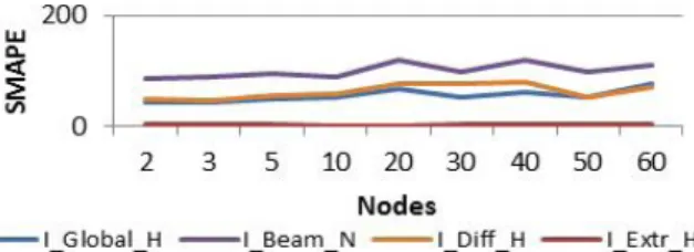
advan-tageous combination of parameters. The parameters that have presented the higher influence on the results are: the number of nodes in the ANN’s hidden layer, and the training limit, i.e. the amount of training data. Figure 1 presents the results of the variation of the number of intermediate layer nodes, when using each of the four fields of solar irradiance independently for the forecast, namely: I_Global_H, I_Beam_N, I_Diff_H and I_Extr_H.

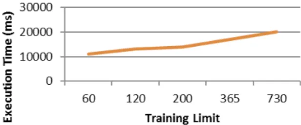
Figure 2 presents the SMAPE error variation for different amounts of training data.

Figure 1. Forecasting error for different numbers of intermediate nodes, for each solar field

From Figure 1 and Figure 2 it is visible that the best combination would be to use 3 intermediate nodes with a training limit of 120. Figure 1 shows that the increase of the hidden layer nodes instigates an increase of the forecasting error values in three from the four solar intensity data types. 3 nodes is the number that presents the

best overall results for the four fields. Regarding the training limit, one can see from Figure 2 that the SMAPE

values stabilize after the value of 120. This means that it is irrelevant to include a larger amount of training data,

(10)

Tiago Pinto, Luis Marques, Tiago M. Sousa, ADCAIJ: Advances in Distributed Computing Pinto et al. ADCAIJ Submission Instructions Guidelines

11

Figure 1 – Forecasting error for different numbers of intermediate nodes, for each solar field

From Figure 1 and Figure 2 it is visible that the best combination would be to use 3 intermediate nodes with a training limit of 120. Figure 1 shows that the increase of the hidden layer nodes instigates an increase of the forecasting error values in three from the four solar intensity data types. 3 nodes is the number that presents the best overall results for the four fields. Regarding the training limit, one can see from Figure 2 that the SMAPE values stabilize after the value of 120. This means that it is irrelevant to include a larger amount of training data, as the increase in training execution time does not bring any added value for the quality of the forecasts.

Figure 2 – Forecasting error for different amounts of training data, for each solar field

Thus 3 intermediate layer nodes, and a training limit of 120 are the values that are used for all ANN based methodologies. Table 1 shows the SMAPE error values of the first methodology (M1).

I_Glob_H I_Beam_N I_Diff_H I_Extr_H M1 - SM1 39,81 81,49 38,24 1,16 M1 - SM2 37,22 76,19 47,68 7 M1 - SM3 43,67 81,82 34,6 8,16 M1 - SM4 40,14 - - -

Table 1 – SMAPE error values obtained in the forecasts using M1 (with the last 4 periods

In SM4 only the I_Glob_H field is forecasted, therefore, Table 1 does not show the error value concern-ing the other solar intensity fields. For M1, one can see that the best results in forecastconcern-ing the I_Glob_H

Figure 2. Forecasting error for different amounts of training data, for each solar field

Thus 3 intermediate layer nodes, and a training limit of 120 are the values that are used for all ANN based methodologies. Table 1 shows the SMAPE error values of the first methodology (M1).

Table 1. SMAPE error values obtained in the forecasts using M1 (with the last 4 periods) I_Glob_H I_Beam_N I_Diff_H I_Extr_H

M1 - SM1 39,81 81,49 38,24 1,16

M1 - SM2 37,22 76,19 47,68 7

M1 - SM3 43,67 81,82 34,6 8,16

M1 - SM4 40,14 - -

-In SM4 only the I_Glob_H field is forecasted, therefore, Table 1 does not show the error value concerning the other solar intensity fields. For M1, one can see that the best results in forecasting the I_Glob_H field are achieved when using the four solar intensity fields at the same time, for the forecasting process (SM2). Table 2

shows the SMAPE forecasting results, referring to the second methodology (M2).

Table 2. SMAPE error values of the M2 methodology I_Glob_H I_Beam_N I_Diff_H I_Extr_H

M2 - SM1 34,02 74,81 46,14 2,69

M2 - SM2 54,57 100,6 47,43 7,86

M2 - SM3 47,43 92,87 92,81 9,92

M2 - SM4 46,27 - -

-From Table 2 it is visible that, concerning the forecast errors’ analysis using the last 24 periods, using only one solar field (SM1) leads to obtaining better predictions. Table 3 presents the results of M3.

Table 3. SMAPE error of the forecasts using the last 7 days – M3 I_Glob_H I_Beam_N I_Diff_H I_Extr_H

M3 - SM1 44,4 83,08 61,4 0,52

M3 - SM2 48,96 74,28 49,72 8,67

M3 - SM3 53,19 109,87 49,03 9,91

(11)

-95 Tiago Pinto, Luis Marques, Tiago M. Sousa,

© Ediciones Universidad de Salamanca - cc by From Table 3, concerning the forecasts errors’ analysis with the last 7 days, we concluded that using one solar field (SM1) leads to obtaining better forecasts, precisely because it gets the best global solar intensity

forecast.

Finally, to conclude the ANN tests analysis, in the first methodology, using the last 4 periods it was conclud

-ed that using the 4 solar fields obtain better forecasts, with and error of 37,22 for I_Glob_H parameter. In the second methodology, using the last 24 periods best forecasts are obtained using one solar field, with an error of 34,02 for the parameter I_Glob_H. Finally, the third methodology using the same period of last week, obtains better predictions using one solar field, with an error of 44,4 for the parameter I_Glob_H. The methodology

which achieved better forecast, as can be seen by calculating the error, was the second, using the last 24 periods,

and the first sub-methodology, using only the I_Glob_H field as training data, while ignoring the other (M2 –

SM1), with a SMAPE value of 34,02.

4.2. SVM methodologies

Similarly to the ANN based methodologies, more than one approach has been considered, regarding the input

data to train the SVM. Two solutions have been implemented, which use as input:

• SVM_M1 - the same period in the last days, i.e., using data from the same hour that is forecasted, but in

the last days preceding the day to forecast;

• SVM_M2 - last hours, i.e. use the latest hours before the hour of the day that is being forecasted. Considering the conclusion taken from the performance of the ANN based approach that the use of the I_Glob_H field by itself leads to better forecasting results, and given the intrinsic nature of SVM, which as

-sumes a single data series prediction; only the historical data of the I_Glob_H field is used by the SVM based

approaches.

Sensitivity tests have been performed in order to determine the best parameterizations for the SVM

ap-proach. The most influential parameters on the results are: the kernel function, the angle of the kernel function – σ, and the amount of training data – training limit. Regarding the kernel functions, as mentioned before, the most suitable kernel functions for time series prediction are the RBF and eRBF kernels; therefore, these two kernels have been used.

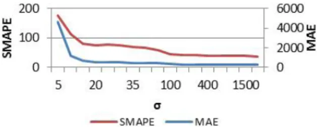
Figure 3 and Figure 4 present the evolution of the MAE and SMAPE error values for different training limits

and σ respectively, when using the SVM approach with the RBF kernel.

(12)

Tiago Pinto, Luis Marques, Tiago M. Sousa, ADCAIJ: Advances in Distributed Computing Figure 4. Forecasting error for different kernel function angles, when using the SVM approach

with the RBF kernel

From Figure 3 and Figure 4 it can concluded that the use of the SVM methodology with the RBF kernel achieves the best results with a training limit of 25 and σ equal to 1000. Figure 5 and Figure 6 present similar sensitivity analysis results for the SVM approach using the eRBF kernel.

Figure 5. Forecasting error for different training limits, when using the SVM approach with the eRBF kernel

Figure 6. Forecasting error for different kernel function angles, when using the SVM approach with the eRBF kernel

From Figure 5 and Figure 6 can be concluded that the SVM methodology using the eRBF kernel reaches its optimal performance with the training limit value of 25 and σ of 10. Table 4 presents the Standard Deviation (SD), MAE and SMAPE error values of the SVM methodology for the I_GLOB_H solar irradiance field.

Table 4. SMAPE error of the forecasts using the last 7 days – M3

Methodology Kernel SD MAE SMAPE

SVM_M1 RBF 229,5 270,77 38,37

eRBF 301,56 328,97 48,99

SVM_M2 RBF 317,12 179,7 23,36

eRBF 287,4 151,62 21,48

From Table 4 it is visible that the second methodology (SVM_M2) achieves better forecasting results than SVM_M1, for both kernel functions. Additionally, despite the use of the RBF kernel being able to provide better results with the SVM_M1 methodology, the eRBF kernel was able to achieve better results with the SVM_M2

(13)

methodology, and also the global best ones of the SVM based methodologies. Therefore, the conclusion is that

using SVM_M2 with the eRBF kernel is the solution capable of reaching the best solar irradiance forecasts. Finally, comparing the SVM approach with the ANN methodologies (which best result has been achieved by the M2 – SM1 methodology, with a SMAPE value of 34,02), one can conclude that the SVM_M2 methodology with the eRBF kernel is the best overall approach, with a SMAPE of 21,48.

4.3. Hybrid methodologies

The huge differences of forecasting quality that have been observed in the previous tests when using different

methodologies, support the fact that the way data is looked at when analysing the historic, is essential for the forecasting process. For this reason, a novel approach is proposed, which aims at filtering and arranging the data

automatically, selecting only the data that is most relevant for each case, so that the disparity of historic values

can be reduced, and only the most influential and constant data is used for the training process.

The data filtering process is conducted by applying a clustering algorithm, k-means, which groups the data

into different clusters according to the values similarity. Several different approaches for splitting the historical

data have been experimented, namely, by year, by season, by month, and by periods of the day.

In order to evaluate the best grouping of the clustering mechanism CDI (Clustering Dispersion Indicator) is used. CDI calculates the disparity of the values that are grouped in the same cluster, therefore, the smaller the value is, the most constant the values of each cluster are, i.e. the used data set becomes less volatile. Figure 7 presents the CDI values that have been achieved, for a different number of clusters, for each different grouping approach.

Figure 7. CDI value for each data grouping approach according to number of clusters

From Figure 7 it becomes conclusive that the division by periods of the day is the best one, as it is clearly below all other approaches for all numbers of clusters. The splitting by periods of the day means that data is

divided by hours of the day. In the current case, of solar intensity forecasting, the data profile for each day is

similar throughout the time: null values during night-time; an increasing tendency during the morning; the

peak values are found during the midday hours; and finally a decreasing tendency until nightfall. This grouping process assures that, for instance the night-time null values are all placed in one group, the peak hours of solar

irradiance in another, and so on. This way, when forecasting a solar irradiance value for a certain hour of the day, only the data concerning the most similar hours are used, refraining from using irrelevant (or even misleading) data from the training process.

The number of clusters that have been used for these tests is 6. A careful balance between the number of clusters and the possible gain by using them must be taken into account. Note that using a high number of clus

-ters means keeping a smaller amount of historic data for the training process. On the other hand, the higher the number of clusters is, the more refined the grouping is. For this reason, one must realize at which point the use

(14)

of additional clusters stops being advantageous. This is usually verified by determining the point in which the CDI curve starts stabilizing and decreasing less drastically. For the current case the ideal number is 6 clusters,

as can be seen by theByPeriodsline of the graph of Figure 7. Figure 8 presents the clustering results of the

By-Periods approach using five clusters, for twelve exemplification days (1st day of each month of the year 1999).

Figure 8. Clustering results of the ByPeriods approach, for six clusters

From Figure 8 it is visible that hours with similar solar intensity values are grouped in the same cluster. This is true even for days with very different values of solar intensity, such as days during the winter and during

the summer. Since the solar tendency is similar during all year, all days are successfully classified in clusters that join nightly hours (null values), peak intensity hours, and hours with intermediate solar intensity. Using

the separation of hours provided by the clustering process, the forecasting process is adapted, so that only the

hours from previous days that are classified in the same cluster are considered as training data by the ANN and

the SVM approaches.

Table 5 presents the comparison between the SMAPE error values of the best ANN and SVM approaches, with and without the use of the proposed filtering process.

Table 5. SMAPE error of the forecasts of the best ANN and SVM methodologies with and without the use of the proposed clustering based filtering process

Methodology Kernel Without Clustering With Clustering

ANN M2_SM1 - 34,02 29,71

SVM_M2 RBF 23,36 21,84

eRBF 21,48 19,23

From Table 5 it is visible that the use of the data filtering process implicates an increase in the forecasting quality of the proposed ANN and SVM approaches. The decrease of the error values is originated by an ade -quate selection of the data that is used for the training process.