Explaining long-term trends in groundwater
hydrographs
Ferdowsian, R.1 and D.J. Pannell2 1
Department of Agriculture and Food, Western Australia 2
School of Agricultural and Resource Economics, University of Western Australia Email: [email protected]
Abstract: An ability to understand and interpret changes in groundwater levels is essential for sound
management of groundwater resources. Various statistical methods have been developed to explain hydrograph trends. Most of these operate on the assumption that groundwater trends are linear or best represented by short linear segments. However there is clear evidence that many hydrograph trends are non-linear. For example, as the groundwater level changes, the area of groundwater discharge may change, dynamically feeding back and altering the trend rate of change.
The long-term underlying trend of groundwater level over time may or may not be linear. Three types of long-term trends may be observed:
• We may observe a rising trend that reduces over time and is a common feature of local groundwater flow systems. In these cases, as groundwater level rise, the hydraulic gradient and the rate of flow (discharge) both increase. The result is that the rate of groundwater rise falls systematically over time.
• There are cases where the long-term trend in groundwater level is linear. This is usually the case where aquifers are intermediate to regional, have relatively higher recharge to discharge ratios, very little hydraulic gradient to generate significant flow and groundwater levels are well-below the soil surface.
• Occasionally we may observe an increasing rate of groundwater rise. This may be observed where stagnant aquifers are segmented by obstacles (eg basement highs). In such cases each segment will rise until the area of discharge has increased or groundwater finds a convenient flow path to spill into the lower part of the aquifer. From that time, the lower segment, receiving water from another segment, will have an increasing rate of groundwater rise, at least for a period.
We present three models for statistically estimating non-linear trends in groundwater levels. The first model is an autoregressive model, in which a past moving average of the dependant variable is included as an explanatory variable. This approach is useful when regular and frequent water-level data is available, although it has a few shortcomings. The second model uses time-related spline functions in the GenStat statistics package. The third model includes a log time function to capture the non-linear trend.
Both, the spline and log time models are easy to use and produce realistic trend lines. The spline function is a subjective method as the number of splines needs to be selected. The advantage of the log time model over the spline method is that it is not subjective and does not need special software; the solver function of Microsoft Excel may be used to do the analysis. We provide detailed guidance on performing the spline and log time models.
1. INTRODUCTION
Fresh groundwater is a valuable resource while saline groundwater may be a threat to natural resources. In both cases, monitoring and interpreting changes in groundwater levels is essential for management. Hydrographs show changes in groundwater levels over time and are often the most important source of information about the hydrological and hydrogeological conditions of aquifers. The pattern of water-level change in a hydrograph is governed by physical characteristics of the groundwater flow system, the rainfall pattern and the interrelation between recharge to and discharge from an aquifer. Water level changes in a hydrograph can also be caused by other management options such as extraction, irrigation and land use change.
Ferdowsian et al. (2001a) presented a new statistical approach for analysing hydrographs, called HARTT
(Hydrograph Analysis: Rainfall and Time Trends). The method is able to distinguish between the effect of rainfall fluctuations and the underlying trend of groundwater levels over time. Rainfall is represented as an accumulation of deviations from average rainfall and the lag between rainfall and its impact on groundwater explicitly represented. Ferdowsian and Pannell (2001b) showed how to adapt the approach to differentiate between atypical rainfall events, time trends, and the impacts of managements, such as changes in land use, pumping, and drains.
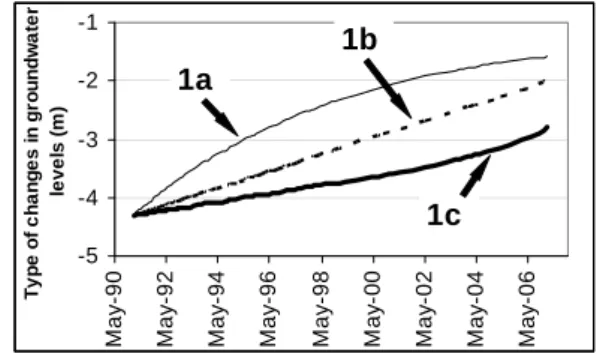
The short-term underlying trend of groundwater level over time is often linear. Three types of long-term trends may be observed (Figure 1). Line 1a represents a rising trend that reduces over time and is a common feature of local groundwater flow systems. In these cases, as groundwater level rise, the hydraulic gradient and the rate of flow (discharge) both increase. The result is that the rate of groundwater rise falls systematically over time.
Line 1b represents a case where the long-term trend in groundwater level is linear. This is usually the case where aquifers are intermediate to regional, have relatively higher recharge to discharge ratios, very little hydraulic gradient to generate significant flow and groundwater levels are well-below the soil surface. Line 1c, represents the case with an increasing
rate of groundwater rise. This may be observed where stagnant aquifers are segmented by obstacles (eg basement highs). In such cases each segment will rise until the area of discharge has increased or groundwater finds a convenient flow path to spill into the lower part of the aquifer. From that time, the lower segment, receiving water from another segment, will have an increasing rate of groundwater rise, at least for a period.
1.1 Merits of detecting the relevant trend
Detecting and quantifying the long-term trend of groundwater rise or fall is valuable for many reasons: 1. It sheds light on the hydrogeological processes operating at the site;
2. It helps us to predict the future degree of threat to natural resources; 3. It helps us to predict the extraction capacity of water resources;
4. It helps us to understand the impact of past land use and water management; and 5. It prevents the risks associated with projecting a linear trend too far into the future.
In this paper we present three methods for estimating the behaviour of groundwater trend lines in the long-term. We describe the advantages and disadvantages of each method and show examples of their application.
2. METHOD
The method proceeds in two stages. In stage 1, the standard HARTT method (Ferdowsian et al, 2001a) is
used to estimate the time-lag between accumulative residual rainfall (ARR) and its impact on groundwater. Two forms of accumulative residual rainfall may be used (Ferdowsian et al, 2001a):
The first was accumulative monthly residual rainfall (AMRR; mm): -5 -4 -3 -2 -1
May
-90
May
-92
May
-94
May
-96
May
-98
Ma
y
-0
0
May
-02
May
-04
May
-06
T
yp
e o
f
ch
an
g
es
in
g
ro
u
n
d
w
at
er
le
v
e
ls
(
m
)
1b 1a
1c
Figure 1:Three possible shapes for trend lines
-5 -4 -3 -2 -1
May
-90
May
-92
May
-94
May
-96
May
-98
Ma
y
-0
0
May
-02
May
-04
May
-06
T
yp
e o
f
ch
an
g
es
in
g
ro
u
n
d
w
at
er
le
v
e
ls
(
m
)
1b 1a
1c
=
−
=
ti
j j i
t
M
M
AMRR
1
,
)
(
(1)where Mi,j is rainfall in month i (a sequential index of time since the start of the data set) which corresponds
to the jth month of the year,
M
j is mean monthly rainfall for the jth month of the year, and t is monthssince the start of the data set.
The second was accumulative annual residual rainfall (AARR; mm):
=
−
=
ti i
t
M
A
AARR
1
)
12
/
(
(2)where
A
is mean annual rainfall.In stage two, we estimate a regression model explaining groundwater level as a function of ARR, time and a third variable, which varies between the three models presented here.
2.1. Autoregressive model with the dependant variable’s past moving average
The first method is a general autoregressive model with the dependant variable’s past moving average (autoregressive moving average = ARMA) included as the third variable (Greene, 1993). The advantage of this method is that the non-linear trend is estimated as a function of past groundwater levels, which is not the case in the next two methods. This method is applicable when regular and frequent water-level data is available.
The regression model was:
Deptht = k0 + k1 × ARRt- L1 + k2 ×t + k3 ×MAt-L2 (3)
where Depth is depth of groundwater below the ground surface, t is months since observations commenced, L1 is lengths of time-lag (in months) between rainfall and its impact on groundwater, MA is past moving
average of groundwater levels, L2 islengths of time-lag (in months) between past moving average and the
present groundwater levels and k0, k1, k2 and k3 are parameters to be estimated. Parameter k0 is approximately equal to the initial depth to groundwater, k1 represents the impact of above- or below-average rainfall on the
groundwater level, k2 is the linear trend rate of groundwater rise or fall over time and k3 represents the impact
of past groundwater levels. The expression k2 ×t + k3 ×MAt-L2represents the long-term trend of groundwater
rises or falls over time.
The non-linear trend estimated using this method may not vary monotonically. It is likely to rise and fall according to past rainfall patterns. This may or may not be considered a problem, depending on the purpose of the analysis.
A decision is required regarding the time frame over which the moving average variable (MA) is calculated.
A longer calculation period reduces the noise associated with seasonal fluctuations in groundwater levels. Here we use one month. The next challenge is to select a suitable delay between the dependant variable and its past moving average. The shortest delay will result in the best fit, but will mask the impacts of other factors (rainfall and time). In this example, we have used a delay of one year.
2.2. Spline functions
The second method is to use time-related spline function. Splines are functions built from segments of polynomial. The pieces are constrained to be smooth where they join (known as “knots”). We have found that a quadratic polynomial that involves the square of time (t) to provide a good fit for long-term
hydrographs. Here is an example of a quadratic polynomial equation.
a × t2 + b × t + c (4)
The GenStat statistics software (GenStat 2008) provides a facility to estimate spline functions. We obtained a good result by estimating groundwater level as a linear relation of ARR and a splined quadratic polynomial function for the time. The function was expressed as:
where Depth is depth of groundwater below the ground surface, t is months since observations started, L is
lengths of time-lag (in months) between rainfall and its impact on groundwater.
The expression SSPLINE (Monitoring_date: 2) is the spline submodel. GenStat estimates the value of this
submodel as well as the parameters k0, k1 and k2.
The spline function is a subjective method as the number of splines needs to be selected. Another drawback of the method is that its trend line is made-up of two or more segments. This makes it difficult to use the approach for prediction of the future trend.
2.3. The log time method
The regression model for this method is:
Deptht = k0 + k1 × ARRt- L + k2 ×t + k3 × ln (k4 × (t+ k5)) (6) where Depth is depth of groundwater below the ground surface, ARR is accumulative residual rainfall, t is
months since observations started, ln is the natural logarithm function, L is time-lag (in months) between
rainfall and its impact on groundwater, and k0, k1, k2, k3, k4 and k5 are parameters to be estimated. Parameter k0 is approximately equal to the initial depth to groundwater and k1 represents the impact of above- or
below-average rainfall on groundwater level. The expression k2 ×t + k3 × ln (k4 × (t+ k5)) represents the long-term trend of groundwater rise or fall over time. We can use Solver tool in Microsoft Excel to estimate the k’s
based on minimising the sum of squared errors: ∑ (Fitted-Actual)2.
2.4. Advantages and disadvantages of the three methods
Relative to the ARMA method, the spline functions and log time approaches have the following advantages:
• They do not need subjective selection of the period for estimating the moving average and its lagged impact;
• They can cope better with missing data because of irregular monitoring; and
• They produce a smoother trend, and may be better suited for predicting future groundwater levels. In the spline function approach, if the number of splines exceeds two, it too becomes a curve fitting method and tends to lose its predictive value. Section 4 gives more details about the advantages and disadvantages of the three methods.
3. RESULTS AND DISCUSSION
Here we show three case studies. The first case shows the application of all three methods. The second and the third cases show application of spline function and log time models.
3.1. Case 1
Case 1 is for bore Ah31. This bore is located 12km east of Frankland in Western Australia and has 18 years of groundwater data. The bore has a trend similar to line 1a in Figure 1. Figure 2 shows the raw groundwater data for bore Ah31 and the related ARR with one month delay. We can see that groundwater levels have risen despite the ARR having a falling trend (a decline in long-term rainfall).
The bore is in a local-scale groundwater flow system. Based on Darcy’s Law, the rising trend reduces as groundwater levels rise. All the three models explained the variables well (R2 > 0.9;
Table 1).
-10 -9 -8 -7 -6 -5 -4 -3 -2 -1 0
7/
05/
90
6/
05/
92
6/
05/
94
5/
05/
96
5/
05/
98
4/
05/
00
4/
05/
02
3/
05/
04
3/
05/
06
G
rou
ndwat
er
lev
els
(
m
)
-500 0 500 1000 1500 2000 2500 3000 3500 4000 4500
A
RR (
m
m
)
Actual GW levels
Accummulative residual rainfall (AAR)
Figure 2: Unprocessed groundwater level data for bore Ah31 and the ARR with one month delay.
Table 1: The log time method explained the changes in groundwater levels of bore Ah31 better than the
other two methods.
Method Sum of squared residuals R2
Log time method * 1.352 0.930
Spline functions with 2 degrees of smoothing (two segments) * 1.609 0.912 Autoregressive model with 1-year delayed moving average
water-level * 1.898 0.902
* Note that p-value for all parameters (k0, k1, k2 and k3) were <0.001. Estimated long-term trend lines using each of the
three methods are shown in Figure 3. Note that these are not fitted values, as they show only the time-related variables. The spline and log time approaches result in similar estimates of the long-term trend, with groundwater rising at a
decreasing rate over time in each case. The autoregressive model results in a fluctuating trend line (as explained earlier; Figure 3). Its overall trend is more nearly linear than the other two, and, in this example, it may over-predict the rate of groundwater rise in future periods.
3.2. Case 2
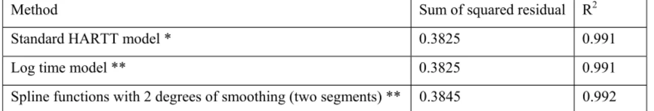
The second case is for a bore (Koj 1d88), in a Tertiary sand plain (70km north-east of Albany in Western Australia) within an intermediate groundwater flow system. This bore is in a stagnant aquifer (low hydraulic gradient and flow) and from experience was expected to have a linear long-term trend. Figure 4 shows the actual groundwater level data, impact of accumulative residual rainfall as well as the trend line estimated using a standard HARTT model (k0 + k1 × ARRt- L + k2 ×t; Ferdowsian et al., 2001a). This model explained
99% of the variance (Table 2).
In such stagnant aquifers a standard HARTT model can estimate the long-term trend and there are fewer added values in use of the spline function or log time approaches. For example, the
k3 parameter of the log time model was not
significantly different from zero (p-value was
0.6628), so the model collapsed to the standard HARTT model.
Table 2: The percentage of variance accounted for by HARTT and GenStat methods were more than 99.
Method Sum of squared residual R2
Standard HARTTmodel * 0.3825 0.991
Log time model ** 0.3825 0.991
Spline functions with 2 degrees of smoothing (two segments) ** 0.3845 0.992 * Note that p-value for the standard HARTT model parameters (k0, k1 and k2) were <0.001.
** Note that p-value for k0, k1 and k2 parameters of the log time and spline models were <0.001 but p-value for k3 was >0.5.
-7 -6 -5 -4 F eb-9 1 F eb-9 3 F eb-9 5 Fe b-97 Feb -9 9 Fe b -0 1 Fe b -0 3 Fe b -0 5 F eb-07 D e pt h to gr o un dw at e r ( m )
Trend by spline function Actual water levels Trend by Ln
Trend by moving average
Figure 3:The long-term trend lines estimated for case 1 using each of the three methods.
-7 -6 -5 -4 F eb-9 1 F eb-9 3 F eb-9 5 Fe b-97 Feb -9 9 Fe b -0 1 Fe b -0 3 Fe b -0 5 F eb-07 D e pt h to gr o un dw at e r ( m )
Trend by spline function Actual water levels Trend by Ln
Trend by moving average
Figure 3:The long-term trend lines estimated for case 1 using each of the three methods.
Bore Koj 1d88
-11 -10 -9 -8 -7 -6 -5 A ug 87 A ug 89 Au g 9 1 Au g 9 3 A u g 95 Au g 9 7 A u g 99 A u g 01 A u g 03 A u g 05 A u g 07 Gr ou nd w ate r le ve ls (m ) -0.5 0 0.5 1 1.5 2 2.5 Imp ac t o f A R R (m)
Actual GW levels Trend
Impact of ARR
Figure 4:The raw groundwater level data for bore Koj
1d88, the trend (based on standard HARTT method) and the impact of ARR.
3.3. Case 3
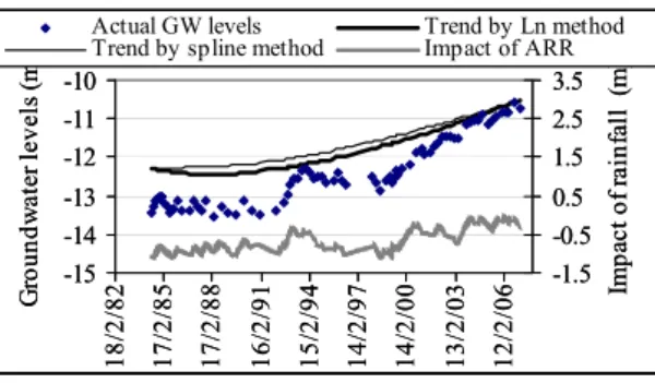
Case 3 looks at groundwater level changes in bore MB2d. This bore which is 66km north-east of Esperance in Western Australia, is in a segmented stagnant aquifer in a Tertiary sand plain. It has 24 years of groundwater level data. There are basement highs in this sand plain that result in the aquifer being interrupted and partitioned. As groundwater levels rise, groundwater finds a convenient flow path to spill into the lower segment. This will cause the lower segment to show a trend of increasing rate of groundwater rise. Bore MB2d is located in one of these lower segments. We note the groundwater level in MB2d has risen at an increasing rate in recent years and the increasing rate cannot be fully explained by changes in rainfall (Figure 5).
Figure 5 shows groundwater level data for bore MB2d. Analysis with the standard HARTT model with different lags indicates that there was a three-month delay between the monthly rainfall and its impact on groundwater levels.
Eighty-nine percent of the variance could be explained using the HARTT model (Table 3). The spline and log time models each explained 95% of variation in groundwater levels (Table 3). Figure 5 shows the impact of ARR (with three months delay) as well as the two trend lines (for spline and log time models). Both of the non-linear models captured the long-term trend well, showing the recent rise in groundwater levels following a period of approximately static levels.
Table 3: Statistical analysis of groundwater level for bore MB2d and the power of the log time and spline
models to show the variation.
Method Sum of squared residual R2
Standard HARTTmodel * 4.967 0.89
Log time model* 1.788 0.95
Spline functions with 2 degrees of smoothing (two segments)* 3.587 0.95 * Note that p-value for all selected parameters were <0.001.
4. DISCUSSION AND CONCLUSIONS
We have presented three models for statistically estimating non-linear trends in groundwater levels. The first model is an autoregressive model, in which a past moving average of the dependant variable is included as an explanatory variable. There are a few challenges to use the approach for prediction of the current and future trends:
• It is a subjective method because a decision is required regarding the time frame over which the moving average variable is calculated.
• The next challenge is to select a suitable delay between the dependant variable and its past moving average.
• The non-linear trend estimated using this method may not vary monotonically. It is likely to rise and fall according to past rainfall patterns. This may or may not be considered a problem, depending on the purpose of the analysis.
The second model uses time-related spline functions in the GenStat statistics package. This model is easy to use and produces realistic trend lines. The spline function method is also subjective as the number of splines needs to be selected. Another drawback of the method is that it requires specialized statistics package. The third model includes a log time function to capture the non-linear trend. This model is also easy to use and produces a realistic trend line. The advantage of the log time model over the spline method is that it is not a subjective model and it does not need special software; the solver function of Microsoft Excel may be used to do the analysis. We provide detailed guidance on performing the spline and log time models.
Figure 5:Groundwater level data for bore MB2d and the
impact of ARR
-15 -14 -13 -12 -11 -10
18
/2
/82
17
/2
/8
5
17
/2
/8
8
16
/2/
91
15
/2/
94
14
/2/
97
14
/2/
00
13
/2
/03
12
/2
/06
G
rou
ndw
at
er
le
ve
ls
(m
)
-1.5 -0.5 0.5 1.5 2.5 3.5
Im
pa
ct
o
f ra
in
fa
ll
(m
)
Actual GW levels Trend by Ln method Trend by spline method Impact of ARR
ACKNOWLEDGMENTS
We thank Andrew Van Burgel from the Department of Agriculture and Food, Western Australia, and Michael Burton from the University of Western Australia for statistical assistance. Acknowledgement is extended to Richard George for his comments on a draft of this paper and to John Simons for providing groundwater level data for the site near Esperance.
REFERENCES
Ferdowsian, R., Pannell D.J., McCarron, C., Ryder A. and Crossing, L. (2001a), Explaining Groundwater Hydrographs: Separating Atypical Rainfall Events from Time Trends. Australian Journal of Soil
Research. 39, 861-875.
Ferdowsian, R. Pannell D.J. (2001b), Explaining trends in groundwater depths: distinguishing between atypical rainfall events, time trends, and the impacts of treatments. MODSIM 2001 Congress Proceedings,
Canberra, 10-13 December 2001. PP. 549-554 (Modelling and Simulation Society of Australia and New
Zealand INC)
Greene, W.H. (1993), Time-Series Models. In ‘Economic analysis’. (Second edition) pp.549-578.
(Prentice-Hall. Inc. New Jersey)