Critical data points retrieving method for big sensory data in wireless sensor networks

R E S E A R C H

Open Access

Critical data points retrieving method for

big sensory data in wireless sensor networks

Tongxin Zhu

, Siyao Cheng

, Zhipeng Cai

and Jianzhong Li

Abstract

With the development and widespread application of wireless sensor networks (WSNs), the amount of sensory data grows sharply and the volumes of some sensory data sets are larger than terabytes, petabytes, or exabytes, which have already exceeded the processing abilities of current WSNs. However, such big sensory data are not necessary for most applications of WSNs, and only a small subset containing critical data points may be enough for analysis, where the critical data points including the extremum and inflection data points of the monitored physical world during given period. Therefore, it is an efficient way to reduce the amount of the big sensory data set by only retrieving the critical data points during sensory data acquisition process. Since most of the traditional sensory data acquisition algorithms were only designed for discrete data and did not support to retrieve critical points from a continuously varying physical world, this paper will study such a problem. In order to solve it, we firstly provided the formal definition of theδ-approximate critical points. Then, a data acquisition algorithm based on numerical analysis and Lagrange interpolation is proposed to acquire the critical points. The extensive theoretical analysis and simulation results are provided, which show that the proposed algorithm can achieve high accuracy for retrieving the δ-approximate critical pointsfrom the monitored physical world.

Keywords: Wireless sensor networks, Adaptive sampling, Critical points

1 Introduction

The appearance of wireless sensor networks (WSNs) makes it possible to observe the complicated physical world with low cost. Nowadays, WSNs are widely used in many applications, including military defense [1–4], environment monitoring [5, 6], traffic monitoring [7, 8], and structural health monitoring [9–11]. Meanwhile, the amount of sensory data also grows fast with the wide use of sensor networks. For example, the climate data will exceed 100 PB in 2020 according to the report in [12]. For the Large Hadron Collider in Europe, if all sensory data were recorded, the total amount of the sensory data is nearly 50 EB per day. Similarly, the traffic data, includ-ing GPS data, the monitorinclud-ing data captured by electronic eyes, and so on, also increase rapidly and have already exceeded petabyte annually. Fortunately, not all sensory values are necessary for the users’ analysis in most applica-tions. Some critical data points, such as maxima, minima,

*Correspondence: [email protected]

1School of Computer Science and Tech, Harbin Institute of Technology, 150001 Harbin, China

Full list of author information is available at the end of the article

and flection points in a monitoring process, may be the only ones required by the users. Therefore, the algorithms for retrieving the critical data points from the monitored physical world are quite important for WSNs.

Currently, it supposes that the sensor nodes sense and sample the data from the monitored environment with equal sampling frequency in most of traditional applica-tions, and the sensory data generated by WSNs is regarded as a set of discrete values. Under such assumptions, a great number of query processing techniques on discrete sen-sory data have been proposed, including the curve query processing algorithms [13], aggregation query process-ing algorithms [14–17], top-k query processprocess-ing algorithms [18–20], skyline [21, 22], and quantilen [23, 24] query processing algorithms. Although all the above algorithms are efficient for processing the discrete sensory data, they cannot meet the complicated query requirements given by users and do not support to retrieve the critical data points in current WSNs since only discrete data were considered. For example, in the air pollution monitor-ing application, the users want to estimate the extremum

pollution values and obtain the period when these val-ues appear. In the climate monitoring system, the users may want to know the convexity of the wind velocity or rainfall curve and acquire the inflection points of such curves. The reasons the above query requirements cannot be satisfied by the existing query processing techniques, which only consider the discrete sensory data, are given as follows. First, as pointed out by [25, 26], the moni-tored physical world varies continuously, and the discrete sensory dataset omits many critical points, such as max-ima, minmax-ima, and flection points from the physical world, so that the queries of retrieving critical points cannot be answered since these points do not belong to the discrete sensory dataset. Second, to answer the queries about the convexity, monotonicity, or the positions of critical points, the original data needs to have the continuous first and second derivatives, which cannot be met by the discrete sensory dataset either.

To overcome the above problems, Cheng et al. [26] proposed an adaptive data acquisition algorithm to recon-struct the physical world as much as possible. For any

given error bound, the authors proved that the result

returned by their algorithm is O() approximate to the

monitored physical world, where can be arbitrarily

small. Since the sampling frequency of each sensor is adjusted adaptively according to the variation of the mon-itored physical world, the algorithm proposed by [26] samples few sensory data and saves lots of energy on con-dition that the observation error is guaranteed. However, since the aim of [26] is to reconstruct the physical world, the amount of sensory data acquired by the sensors is still quite large. Considering that many applications may only want to acquire the critical point information, such as as maxima, minima, and flection points, according to the above analysis, therefore, the energy cost of collecting the sensory data from the monitored physical world can be further reduced.

Due to the above reasons, we will study the problem of retrieving the critical points, including the extremum and inflection points, in the sensor networks. In this paper, a novel sensory data acquisition algorithm is proposed based on numerical analysis techniques [27] and Lagrange interpolation [28] in order to retrieve the critical points approximately. Such algorithm can adjust the sampling frequency of sensors adaptively according to the varia-tion of physical world in order to dramatically reduce the amount of sensory data. Furthermore, to evaluate the error of approximate critical points, the formal definitions

of δ-approximate extremum point and δ-approximate

inflection point are firstly provided, where δ denotes

the relative error between the approximate critical point and the exact one. The correctness of the algorithm is proved. In summary, the contributions of this paper are as follows.

1. The formal definitions ofδ-approximate extremum point andδ-approximate inflection point are firstly proposed. The problem of acquiring critical points from the monitored physical world is also defined. 2. Two critical point aware data acquisition algorithms

are proposed based on numerical analysis [27] and Lagrange interpolation [28] techniques. The algorithms can adjust the sampling frequency of the sensors automatically according to variation of the physical world. The correctness of the algorithms is proved and the complexities of the algorithms are analyzed.

3. The extensive simulations on the real data set are carried out. The experimental results show that both of the precision and recall rate of our proposed algorithms are quite high to retrieveδ-approximate extremum point andδ-approximate inflection point from the monitored physical world.

The organization of the paper is as follows. Section 2 gives the problem definition. Section 3 provides the math-ematical foundations of the algorithms. Section 4 pro-poses two critical points aware data acquisition

algo-rithms, to retrieve the δ-approximate extremum point

andδ-approximate inflection point, respectively. Section 5 shows the experimental results. Section 6 discusses the related work of the paper. Finally, section 7 concludes the whole paper.

2 Problem definition

LetNdenote the number of sensor nodes in a given WSN,

andV = {1, 2,· · ·,N}be the set of sensor nodes, where

i(1≤i≤N)denotes the ID of a sensor node.

Suppose that ts andtf denote the start and final time in monitoring the physical world by a WSN, respectively. Therefore, the variation of the physical world monitored

by sensor node i can be regarded as a curve. We use

Si (1 ≤ i ≤ N) to denote such curve. According to

the discussion in [26], the physical world always varies

continuously andSi is smooth enough to have a

contin-uous fourth-order derivative, i.e., Si ∈ C4[ts,tf], where

C4[ts,tf] denotes the set of functions whose fourth-order derivative is continuous in [ts,tf].

In this paper, the critical points considered by us are extremum points and inflection points of the physical

curve Si (1 ≤ i ≤ N). Since Si has the

continu-ous fourth-order derivative according to the above anal-ysis, the extremum points of Si in range [ts,tf] can be denoted byx|S(_i1)(x)=0x∈[ts,tf]

; similarly, the inflection points of Si in [ts,tf] can be denoted by

x|S(_i2)(x)=0x∈[ts,tf]

Since when the critical points will appear in the future is unknown, it requires that the sampling frequency should be infinite to obtain all the critical points of Si exactly, which is almost impossible. Thus, we will study the sen-sory data acquisition algorithm to retrieve the critical points, including the extremum points and the inflec-tion points, approximately. To evaluate the relative error between the approximate critical points and the exact

critical points, the δ-approximate extremum point and

δ-approximate inflection pointare defined as follows.

Definition 1. (δ-approximate extremum points) xi fromSiis called as aδ-approximate extremum point if and only if∃xi∈[ts,tf] satisfying|xi−_xixi| ≤δandS(i1)(xi)=0.

Definition 2. (δ-approximate inflection points) xi is called as aδ-approximate inflection point if and only if

∃xi∈[ts,tf] satisfying thatS(i2)(xi)=0 and|xi_x−_ixi| ≤δ. The intuition of our algorithm is to forecast the first and second derivatives ofSi using the current collected sen-sory data. If the first or second derivative is close to 0, then the sampling frequency increases. Otherwise, we reduce the sampling frequency in order to save energy. Since the physical world varies continuously, it is acceptable to use the history sensory data to forecast the future. The detailed algorithm is presented in Section 4, and the for-mal definition of retrieving the approximate critical points from physical world is given as follows.

Input:

1. The start and final time of monitoring,t0(=ts)

andtf

2. The maximum bound of the sampling frequency of a sensor node,fmax

3. The step-size incrementtand the decrease factor

α

Output:The sets of approximate extremum and inflection points in[ts,tf],X1andX2

We verify that the precision and the recall rate of our algorithms are quite high on condition thatδ-approximate

extremum pointsandδ-approximate inflection pointsare

collected. To improve the readability of the whole paper, the table of the symbols used in this paper is given in Table 1.

3 Mathematical foundations

Lettcdenote the current sampling time,tc−1denote the last sampling time before tc, and t2c−1

2 be the median

of tc and tc−1. For each sensor node i (1 ≤ i ≤ N),

Si

t2c−1 2

should always be sampled besidesSi(tc−1)and

Table 1The meanings of symbols

Symbols Meanings

δ The relative error of the approximate critical point

N The number of sensor nodes in a given WSN

V= {1, 2, ..N} The set of sensors

i The ID of a sensor node

Si The real physical world curve at nodei’s location

Si(t) The sensed value of sensor nodeiat timet

Si(k)(t) The k-order derivative ofSiat timet.

Si(k)(t) The estimation of the k-order derivative ofSiat timet.

X1 The extremum point set returned by our algorithm.

X2 The inflection point set returned by our algorithm.

ts The start time of an observation period

tf The final time of an observation period

tc The current data sampling time slot

fmax The maximum sampling frequency

t The step-size increment

α The decrease factor

Si(tc)in [tc−1,tc]. Based on such operations and a three-point central difference formula [27], the first and second derivatives ofSiatt2c−1

2 can be estimated by the following

two formulas.

Si(1)

t2c−1 2

= Si(tc)−Si(tc−1)

2h −

h2 6S

(3) i

t2c−1 2

(1)

Si(2)

t2c−1 2

= Si(tc)−2Si(t2c−21)+Si(tc−1)

h2 − h

2 12S

(4) i

t2c−1 2

(2)

whereh=t2c−1

2 −tc−1=tc−t2c2−1 denotes the half length of the sampling interval.

The following theorem guarantees that the difference betweenSi(1)

t2c−1 2

andS(_i1)

t2c−1 2

is determined byh2.

Theorem 1.S(_i1)

t2c−1 2

−Si(1)

t2c−1 2

₌ h2 6

S_i(3)

t2c−1 2

−S(_i3)(ξ), whereξ ∈[tc−1,tc].

Proof.Based on Taylor Series, we have

Si(tc)=Si

t2c−1 2

+hS(_i1)

t2c−1 2

+h2

2S (2) i

t2c−1 2

+ h3

Similarly

Let M andm be the maximum and minimum values

of S_i(3)(t) for anyt ∈ [tc−1,tc]. Sinceξ1,ξ2 ∈ [tc−1,tc],

2 . Therefore, according to

Formula (3),we have

S(_i1)

Comparing Formula (3) with Formula (1), we have

The proof of Theorem 2 is similar as that of Theorem 1. These two theorems indicate that the difference between the exact critical points and the approximate ones calcu-lated by Formulas (1) and (2) can be arbitrary small with the decline ofh. estimated by Lagrange interpolation. The sensory values collected by sensor nodei(1≤i≤N)in the last and

cur-The error of such estimation is bounded by cur-Theorem 3, which is very small in practice.

Theorem 3.The errors generated by Formulas (5)

and (6) equal to γ1(t) = S

Proof. According to the property of Lagrange interpo-lation [28], the interpointerpo-lation remainder, denoted byR(x)

satisfies that

R(x)=f(x)−Lf(x)=

f(n+1)(ξ)

wheref(x)is a function whosenth-order derivative is con-tinuous, andLf(x)isn-degree Lagrange interpolation of

f(x), x0,x1,· · ·,xn denote the interpolation points, and ξ ∈[x0,xn].

Therefore, the three-order interpolation remainder of

L1(t)satisfies that

γ1(t)=R(3)(t)=

S(_i4)(ξ)

4! ω

(3) 1 (t)

= S(

4) i (ξ)

4 4t−

t2c−3

2 +tc−1+t2

c−1 2 +tc

(8)

which is the error generated during estimatingS(_i3)(t). The fourth-order interpolation remainder ofL2(t) satis-fies that

γ2(t)=R(4)(t)=

S(_i5)(ξ)

5! ω

(4) 2 (t)

= S(

5) i (ξ)

5 5t−

tc−2+t2c−3

2 +tc−1+t2

c−1 2 +tc

(9)

which is the error generated during estimating S(_i4)(t). Thus, Theorem 3 is proved.

Theorem 3 also verifies that the error generated by Lagrange interpolation estimation is also very small.

4 Critical point aware data acquisition algorithm According to the analysis in Section 3,tcandtc−1denote

the current sampling time and the last one before tc,

respectively.t2c−1

2 is the median time slot oftcandtc−1. Let

fmax be the maximum sampling frequency that a sensor

node can achieve.

Based on such symbols, the whole critical point aware data acquisition algorithm can be divided into two phases. The first one is the initial phase, the sampling frequency in such phase is set to befmaxin order not to omit any crit-ical points. The second one is the maintenance phase; the sampling frequency in such phase is determined accord-ing to the variation of physical world. Since the variation of the monitored physical world in the future is unknown, the posterior estimation is adopted, that is, the history sensory data collected in the current time will be used to estimate the variation of the monitored physical world in the future. Because the physical world always varies con-tinuously, such estimation is acceptable and can achieve high precision.

Specifically, the critical point aware data acquisition algorithm consists of the following five steps.

Step 1. Sample sensory values at timet0,t1

2,t1, where

t1 2 =t0+

1

fmax andt1=t12 + 1

fmax. That is, we

initializehwith the minimum sampling interval _f1

max.

Initializecwith 2, then execute a loop untiltc>tf.

Step 2. Sensor nodei(1≤i≤N)samples the sensory values at timet2c−1

2 andtc, where

t2c−1

2 =tc−1+handtc=t2

c−1

2 +h. Using the sensory

values sampled in the current and last sampling intervals, i.e.,Si(tc−2),Si

t2c−3 2

,Si(tc−1),Si

t2c−1 2

andSi(tc), the Lagrange interpolation polynomial can

be constructed. Therefore,S_i(3)(t)andS(_i4)(t)can be obtained according to Formulas (5) and (6) for

t∈ t2c−3 2 ,tc

andt∈[tc−2,t−c]respectively. Step 3. Call the extremum point retrieving algorithm to obtain the extremum point in current sampling interval and determine the length of the next possible sampling intervalh1, the detailed method is shown in

Section 4.1.

Step 4. Similarly, call the inflection points retrieving algorithm to collect the inflection point and

determine the length of the next possible sampling intervalh2. The detailed algorithm is given in

Section 4.2.

Step 5. Finally, select the minimum one returned by the above two steps to be the adopted length of the next sampling interval, i.e.,h=min{h1,h2}, which

avoids omitting critical points. Go to step 2 with increasingcby 1, and start a new loop untiltc>tf.

The detailed critical point aware data acquisition algo-rithm is shown in Algoalgo-rithm 1.

4.1 Extremum point retrieving algorithm

The extremum point retrieving algorithm has four steps.

Step 1. Sensori(1≤i≤N)estimates the the first derivativeSi(1)

t2c−1 2

based on Formula (1).

Meanwhile,Si(2)

t2c−1 2

should be computed according to Formula (2).

Step 2. Find extremum point in t2c−3 2 ,t2c−21

. If

Si( 1)

t2c−1 2

=0, return the extremum pointt2c−1 2 .

Otherwise, compareSi(1)

t2c−1 2

andSi(1)

t2c−3 2

calculated in last loop. IfSi(1)

t2c−1 2

×Si(1)

t2c−3 2

<0, there must be an extremum point in

t2c−3 2 ,t2c2−1

. Then, retrieve the extremum point by curve tessellation techniques [29].

Algorithm 1: Critical point aware data acquisition algorithm

Input:t0(=ts),fmax,t, the decrease factorα. Output: The set of extremum pointsX1and the set

of inflection pointsX2

1 c←2,h← _f1

5 Construct third order Lagrange interpolation and

estimateS(_i3)(t)

6 Construct fourth order Lagrange interpolation

and estimateS_i(4)(t) (t∈[tc−2,tc])according to the first derivative of the physical world increases or decreases monotonously; therefore, the extremum point may not be contained in the next sampling interval[tc,tc+1], so that the length of the next

sampling interval should be increased in order to save energy. In summary, lethandh1denote the half

length of the current and next sampling interval, then

h1=h+t, wheretis a given constant to denote the

step size increment. 2. IfSi(2)

extremum point is more likely to be included in the next sampling interval; thus, we decrease the length of sampling interval in order to catch the extremum point. Therefore,h1is set to beh1=max

In other situations, h1 maintains the last sampling

intervalh.

Step 4. Returnh1and the extremum point.

The detailed algorithm is shown in Algorithm 2.

Algorithm 2:Extremum point retrieving algorithm

Input:fmax,t,α,Si(tc),Si

6 y₁is determined by curve tessellation techniques

[29] in t2c−3

4.2 Inflection point retrieving algorithm

The inflection point retrieving algorithm also has four steps and can be constructed by similar method shown in above section.

and second derivative

based on Formula (1) and Formula (2).

Step 2. Find inflection point in t2c−3

it. Otherwise, compareSi(2)

we have missed. Then, retrieve the inflection point by curve tessellation techniques [29].

Step 3. There exists three cases that need to be considered when determining the length of the next sampling interval. the second derivative of the physical world increases or decreases monotonously; therefore, the inflection point may not exist in the next sampling interval

[tc,tc+1]. In order to save energy, increasing the

length of the next sampling interval. That is, increase the half length of sampling intervalh2=h+t,

wheretis a given constant to denote the step size increment.

inflection point is more likely to be included in the next sampling interval; thus, we decrease the length of sampling interval in order to catch the inflection point. Therefore,h2is set to beh2=max

In other situations, h2 maintains the last sampling

intervalh.

Step 4. Returnh2and the inflection point.

The detailed algorithm is shown in Algorithm 3. In each sampling interval, the complexity of the above algorithm isO(1) since it only needs to sample two sen-sory values and the first and second derivatives can be calculated in O(1). Therefore, the total complexity of Algorithm 1 is determined by the number of sampling interval it includes.

In the best case, the half length of sampling interval,h,

increasestevery loop. Therefore, there existsO

tf−ts

t

sampling intervals, so that the minimum complexity of the

above algorithm isO

tf−ts

t

.

Algorithm 3:Inflection point retrieving algorithm

Input:fmax,t,α,Si(tc),Si

5 y₂is determined by curve tessellation techniques

[29] in [t2c−3

In the worst case, the sampling frequency is alwaysfmax, so that the maximum complexity of the above algorithm is Ofmax(tf−ts)

. However, the worst case requires that there should exist lots of critical points in [ts,tf], which is rarely happened. Therefore, in practice, the com-plexity of our algorithm is much better than the worst case.

4.3 Discussion: the method for estimating missing critical

points

If the product of the first derivatives oft2c−3 2 andt2

<0, then there

Theorem 4.WhenSi(1)

< 0, there must exist a critical point in t2c−3

2 ,t2c2−1

, since Si has continuous fourth-order derivative. We denote the critical point as

t, t ∈ t2c−3 2 ,t2

c−1 2

. According to the definitions of δ-approximate extremum and inflection points, tc−1 is a δ-approximate critical point if and only if |tc−1−t|

According to Theorem 4, the missing extremum points can be obtained by following three steps.

Step 1. Judge whethertc−1is aδ-approximate

extremum point by Theorem 4. Step 2. Use the the valuesSi(1)

to locate the interval where the approximate extremum point is in. Step 3. Use the Lagrange interpolation polynomial we constructed before to estimate the sampling value of the estimated extremum point.

The detailed algorithm for estimating the missing extremum point is shown in Algorithm 4. As shown in the algorithm, we use the linear function to estimate approx-imate extremum point if the condition in Theorem 4 is not satisfied, and more complicated situation will be con-sidered in our future works. For the missing inflection points, the similarly method can be adopted to retrieve them approximately.

The complexity of Algorithm 4 isO(1). The algorithm only needs to conduct compares and additions which can be calculated inO(1). So the method for estimating these missing critical points is efficient.

Algorithm 4:The algorithm of estimating the missing extremum points

4.4 Discussion: the in-network cooperation and

communication algorithms

The above algorithms are all about single sensor’s sens-ing strategies, which can reduce sensory data. Obviously, when in-network cooperation and communication is con-sidered, the sensory data can be further reduced. Since sensory data is spatially-related, not all the sensors need to transmit their critical points. That is, when two sen-sors are close enough, the critical points of their sensory data may appear at the same time. In this situation, not all the critical points need to be transmitted since they may present the same area. We design an algorithm for the in-network cooperation and communication, which can further reduce the transmitting sensory data and the communication energy.

Firstly, we divide the sensors into clusters according to their positions. We divide the monitored area into squares, whose length of the side isD. The length of the

side Dis given by the users according to the specified

according to the positions. When the distance of two crit-ical points is less than L, only one of the critical points will be transmitted, whereLis a parameter given by the users. The detailed algorithm of in-network cooperation and communication is shown in the Algorithm 5.

This algorithm employs the spatial correlation of the sensors, which can further reduce the transmitting energy. Only simple in-network cooperation and communication is considered in the algorithm, since this paper mainly focuses on requiring critical points by single sensor. In the future work, we will study the in-network cooperation to further reduce the energy consumption.

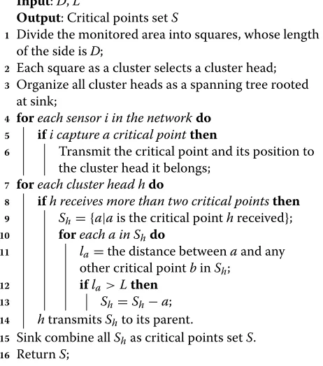
Algorithm 5:The algorithm of in-network cooperation and communication

Input:D,L

Output: Critical points setS

1 Divide the monitored area into squares, whose length of the side isD;

2 Each square as a cluster selects a cluster head;

3 Organize all cluster heads as a spanning tree rooted at sink;

4 foreach sensor i in the networkdo

5 ifi capture a critical pointthen

6 Transmit the critical point and its position to

the cluster head it belongs;

7 foreach cluster head hdo

8 ifh receives more than two critical pointsthen

9 S_h= {a|ais the critical pointhreceived};

10 foreach a in S_hdo

11 la=the distance betweenaand any

other critical pointbinSh; 12 ifla>Lthen

13 S_h=S_h−a;

14 htransmitsS_hto its parent.

15 Sink combine allShas critical points setS.

16 ReturnS;

5 Experiment result

5.1 Experiment setting

We use a simulated network with 200 sensor nodes to evaluate the performance of our sensory data acquisition algorithms. The network is deployed into a rectangular

region with 200×200 m size. The transmission range of

each sensor node is set to be 25 m.

The sensory data of the network comes from a real sen-sor system, where the TelosB mote (http://www.willow.co. uk/TelosB_Datasheet.pdf) is used to acquire indoor tem-perature, humidity, and light intensity continuously with the frequency equaling to 1 Hz, and the light intensity is adopted in the experiments.

5.2 The performance of the algorithm

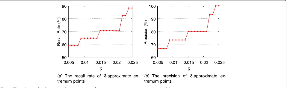
The first group of experiments is going to evaluate the recall rate and precision of our algorithm for retrievingδ -approximate extremum and inflection points. The recall rate equals to the fraction of the exactδ-approximate crit-ical pointsthat are returned. The precision is the fraction of the returned results that are the exactδ-approximate

critical points. They are important parameters to evaluate

the accuracy of the proposed algorithm. In the following experiments, the recall rate and the precision of our algo-rithm were computed, respectively, whileδincreases from

0.005 to 0.025,α = 0.5, andt = 0.5. The experimental

results are presented in Figs. 1 and 2.

From Fig. 1a, b, we can see that the recall rate and

pre-cision of δ-approximate extremum points increase with

the growth ofδ, and both of them are close to a hundred

percent even when δ is quite small. For example, when

δ=0.024, the precision ofδ-approximate extremum point

is 100 % and the recall rate ofδ-approximate extremum

point is close to 90 %. The results in Fig. 2a, b show that the recall rate and precision ofδ-approximate inflection

points are also close to a hundred percent even when

δ is relatively small. The recall rate and precision of δ

-approximate critical points increase with the increase

of δ, since δ is the relative error. When the error is

loose, the algorithm can capture more approximate criti-cal points which leads to higher recriti-call rate and precision. Furthermore, when the relative error is not too large, the algorithm can capture almost all critical points.

In summary, our algorithms can achieve high accuracy in practice.

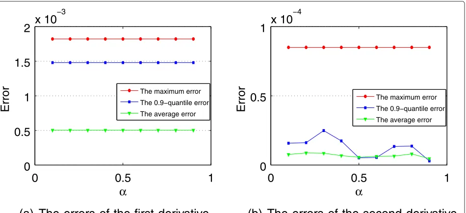
The second group of experiments is to investigate the

impact ofα on the performance of our algorithm. In the

following experiments, the recall rate, the precision, and the errors of the first and second derivatives generated by our algorithm are computed respectively whileαincreases

from 0 to 1,δ = 0.015, andt = 0.5. The experimental

results are presented in Figs. 3 and 4.

Figure 3a, b shows the the recall rate and precision of δ-approximate extremum and inflection points. The recall

rate and precision of δ-approximate inflection points

decrease with the growth ofα; the reason is that the larger αwill omit more inflection points. Besides, the recall rate and precision ofδ-approximate inflection points are still every high even whenαis not very small. For example, the recall rate ofδ-approximate inflection points reaches 96 % whenα =0.1. At the mean time, the recall and precision

rate ofδ-approximate extremum points keep stable and

high enough in practice with the variation ofα. Such recall rate and precision are quite high and can be acceptable in practice.

0.005 0.01 0.015 0.02 0.025 50

60 70 80 90

δ

Recall Rate (%)

(a) The recall rate of δ-approximate ex-tremum points

0.005 0.01 0.015 0.02 0.025 60

70 80 90 100

δ

Precision (%)

(b) The precision of δ-approximate ex-tremum points

Fig. 1The relationship between the accuracies ofδ-approximate extremum points andδ

derivatives are quite small for different α, which indi-cate the high accuracy of our algorithm and also explain why the recall rata and precision of our algorithm are quite high. For example, the average error of the estimated first derivative is less than 10−3and the average and 0.9-quantile errors of the estimated second derivative is about 10−4_.

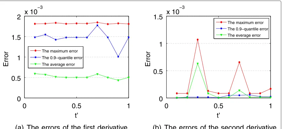
The third group of experiments is to investigate the impact ofton the performance of our algorithm. In the experiments, the recall rate, the precision, and the errors of the first and second derivatives generated by our algo-rithm are calculated, whiletincreases from 0.1 to 1,α = 0.5, andδ=0.015. The experimental results are presented in Figs. 5 and 6.

Figure 5a, b shows that the recall rate ofδ-approximate inflection points is around 90 % and the precision of δ-approximate inflection points decreases with the growth oft, since moreδ-approximate inflection points will be

omitted when t is larger. Although the recall rate and

the precision ofδ-approximate extremum points are lower than δ-approximate inflection points, we still capture a large portion of extremum points.

Figure 6a, b shows the maximum, average, and 0.9-quantile errors of the first and second derivatives

generated by our algorithm whiletincreases. The figures show that all these errors are extremely small, which also verify that our algorithm can achieve high precision on identifying the critical points. For example, the maximum error of the estimated first derivative is only about less than 2×10−3. For the estimated second derivative, most of the errors is less than 0.5×10−4_.

6 Related works

Currently, there exists few published works considering the adaptive sampling in sensor networks. Moreover, none of them could support the requirement of retrieving the critical points from the monitored physical world.

Some adaptive sampling algorithms are proposed for particular applications. For example, the algorithm in [30] is designed for target tracking. Each sensor uses sensory values sensed by its neighbours and itself to predict the target position and adjusts the sampling frequency adap-tively. And [31] introduced an energy efficient algorithm to adjust the sampling frequency in the abnormal event detecting applications. It applies Fourier transform to pre-dict the events and to adjust sampling frequency automat-ically. Since they are designed for particular applications, they have limitation in applying.

0.005 0.01 0.015 0.02 0.025 60

70 80 90 100

δ

Recall Rate (%)

(a) The recall rate ofδ-approximate inflec-tion points

0.005 0.01 0.015 0.02 0.025 20

40 60 80 100

δ

Precision (%)

(b) The precision of δ-approximate inflec-tion points

0

0.5

1

70

80

90

100

α

Recall Rate (%)

δ−approximate extremum points δ−approximate inflection points

(a) The recall rate of

δ

-approximate critical

points

0

0.5

1

60

70

80

90

100

α

Precision (%)

δ−approximate extremum points δ−approximate inflection points

(b) The precision of

δ

-approximate critical

points

Fig. 3The relationship between the accuracies of_δ-approximate critical points and_α

Most of works on adaptive sampling apply prediction models to estimate sensory values instead of sampling them. Jain and Chang [32] uses Kalman filter-based pre-diction model to predict sensory values, if the estimations beyond the acceptable range, they will adjust sampling frequency. However, the prediction ability of Kalman fil-ter is limited, and the estimation error may be large. The prediction method in [33] is Box-Jenkins approach. The main idea of the work is to skip samplings from equal-sampling-frequency and use the forecast ones, which

can adjust the sampling frequency adaptively. However, since the method is based on equal-sampling-frequency, its accuracy is even worse than the EFS method. The work in [34] proposed a heuristic adaptive sampling algo-rithm for a glacial sensor network. Each sensor locally adjusts its sensing frequency based on the linear regres-sion forecasting model. Such method reduces the energy cost of acquiring sensory data since the forecasting model is sufficiently utilized. However, the forecasting ability of the linear regression model is limited, and it

0

0.5

1

0

0.5

1

1.5

2

x 10

α

Error

The maximum error

The 0.9−quantile error

The average error

(a) The errors of the first derivative

0

0.5

1

0

0.5

1

x 10

α

Error

The maximum error

The 0.9−quantile error

The average error

0

0.5

1

40

60

80

100

t’

Recall Rate (%)

−approximate extremum points δ−approximate inflection points

(a) The recall rate of

δ

-approximate critical

points

0

0.5

1

60

70

80

90

100

t’

Precision (%)

δ−approximate extremum points δ−approximate inflection points

(b) The precision of

δ

-approximate critical

points

Fig. 5The relationship between the accuracies of_δ-approximate critical points andt

do not consider the problem of retrieving the critical points, either.

As for retrieving critical points in wireless sensor net-works, some published works focus on it. However, few works focus on retrieving extremum and inflection points. The most common critical points they considering is top-k values.

The work in [20] proposed a novel approach for top-k query. The basic idea of it is to use filters for each node, which can filter the unnecessary sensor updates.

Silberstein et al. [19] studied the optimizing top-k queries in wireless sensor networks. The authors proposed to use samples of past sensor readings, which can reduce energy significantly. The work in [18] focuses on the location aware peak value query in sensor networks. It consider the top-k values’ location which is not considered the traditional top-k query. The authors defined LAP-(D,k)query which can find top-k values and the distance between any two values is larger thanD. However, these papers only consider peak values. In face, besides peak

0

0.5

1

0

0.5

1

1.5

2

x 10

t’

Error

The maximum error

The 0.9−quantile error

The average error

(a) The errors of the first derivative

0

0.5

1

0

0.5

1

1.5

x 10

−3

t’

Error

The maximum error

The 0.9−quantile error The everage error

values, the extremum and inflection points are also critical points.

7 Conclusions

This paper studies the critical point aware data

acqui-sition algorithm to obtainδ-approximate extremum and

inflection points from the physical world. We firstly

pro-vide the formal definition of δ-approximate extremum

and inflection points. Then, a data acquisition algorithm is proposed based on numerical analysis and Lagrange interpolation. Such algorithm can adjust the sampling fre-quency of each sensor node adaptively according to the variation of physical world. The correctness of the algo-rithm is proved and the its complexity is analyzed in detail. Finally, the extensive simulations are carried out, which show that our algorithm can achieve high accuracy of retrievingδ-approximate extremum and inflection points from physical world.

Appendix

The construction of the Lagrange interpolation polynomi-als are as follows.

The construction for L1(t): first, let l1k(t) be a k

-Similarly, L2(t) is a fourth-order interpolation

Lagrange polynomial and can be calculated by

L2(t)=Si(tc−2)l20(t)+Si

The authors declare that they have no competing interests.

Acknowledgements

This work was supported in part by the National Basic Research Program of China (973 Program) under Grant No. 2012CB316200, the National Natural Science Foundation of China (NSFC) under Grant No. 61190115, 61370217, the Fundamental Research Funds for the Central Universities under grant No. HIT.KISTP201415, the National Science Foundation (NSF) under Grants No. CNS-1152001, CNS-1252292, the Research Fund for the Doctoral Program of Higher Education of China under grant No. 20132302120045, and the Natural Scientific Research Innovation Foundation in Harbin Institute of Technology under grant No. HIT.NSRIF. 2014070.

Author details

1_{School of Computer Science and Tech, Harbin Institute of Technology,}

150001 Harbin, China.2Department of Computer Science, Georgia State University, 30303 Atlanta, GA, USA.

Received: 24 September 2015 Accepted: 20 December 2015

References

1. Darpa Sensit Program. http://comlab.ecs.syr.edu/workshop2002/files/ RichardButler.pdf

2. S Kumar, D Shepherd, inProc. 4th Int. Conf. on Information Fusion. SensIT: Sensor information technology for the warfighter (Elsevier, 2001), pp. 1–7 3. Z Cai, Z-Z Chen, G Lin, A 3.4713-approximation algorithm for the

capacitated multicast tree routing problem. Theor. Comput. Sci.410(52), 5415–5424 (2008)

4. Z Cai, G Lin, G Xue, inProceedings of 11th Annual International Conference on Computing and Combinatorics 2005 (COCOON). Improved

approximation algorithms for the capacitated multicast routing problem (Springer, Kunming, China, 2005), pp. 136–145

5. M Li, Y Liu, L Chen, Nonthreshold-based event detection for 3d environment monitoring in sensor networks. IEEE Trans. Knowl. Data Eng. 20(12), 1699–1711 (2008)

6. Greenorbs. http://greenorbs.org/

8. B Barbagli, L Bencini, I Magrini, G Manes, A Manes, inProceedings of the 7th International Wireless Communications and Mobile Computing Conference, IWCMC 2011, Istanbul, Turkey, 4–8 July, 2011. A real-time traffic monitoring based on wireless sensor network technologies (IEEE, 2011), pp. 820–825 9. Structural Health Monitoring of the Golden Gate Bridge. http://www.cs.

berkeley.edu/?binetude/ggb/

10. S Kim, S Pakzad, DE Culler, J Demmel, G Fenves, S Glaser, M Turon, in Proceedings of the 6th International Conference on Information Processing in Sensor Networks, IPSN 2007, Cambridge, Massachusetts, USA, April 25–27, 2007. Health monitoring of civil infrastructures using wireless sensor networks (ACM, 2007), pp. 254–263

11. S Kim, S Pakzad, DE Culler, J Demmel, G Fenves, S Glaser, M Turon, in Proceedings of the 4th International Conference on Embedded Networked Sensor Systems, SenSys 2006, Boulder, Colorado, USA, October 31 - November 3, 2006. Wireless sensor networks for structural health monitoring (Springer, 2006), pp. 427–428

12. JT Overpeck, GA Meehl, S Bony, DR Easterling, Climate data challenges in the 21 st century. Science (Washington).331(6018), 700–702 (2011) 13. S Cheng, Z Cai, J Li, Curve query processing in wireless sensor networks.

IEEE Trans. Veh. Technol.64(11), 5198–5209 (2015)

14. J Li, S Cheng, (ε,δ)-approximate aggregation algorithms in dynamic sensor networks. IEEE Trans. Parallel Distrib. Syst.23(3), 385–396 (2012) 15. S Cheng, J Li, in29th IEEE International Conference on Distributed

Computing Systems (ICDCS 2009), 22–26 June 2009, Montreal, Québec, Canada. Sampling based (ε,δ)-approximate aggregation algorithm in sensor networks (IEEE Computer Society, 2009), pp. 273–280 16. S Cheng, J Li, Q Ren, L Yu, inINFOCOM 2010. 29th IEEE International

Conference on Computer Communications, Joint Conference of the IEEE Computer and Communications Societies, 15–19 March 2010, San Diego, CA, USA. Bernoulli sampling based (ε,δ)-approximate aggregation in large-scale sensor networks (IEEE, 2010), pp. 1181–1189

17. Z He, Z Cai, S Cheng, X Wang, Approximate aggregation for tracking quantiles in wireless sensor networks. Theor. Comput. Sci.607, 381–390 (2015)

18. S Cheng, J Li, L Yu, inProceedings of the IEEE INFOCOM 2012, Orlando, FL, USA, March 25–30, 2012. Location aware peak value queries in sensor networks (IEEE, 2012), pp. 486–494

19. A Silberstein, R Braynard, CS Ellis, K Munagala, J Yang, inProceedings of the 22nd International Conference on Data Engineering, ICDE 2006, 3–8 April 2006, Atlanta, GA, USA. A sampling-based approach to optimizing top-k queries in sensor networks (IEEE Computer Society, 2006), p. 68 20. M Wu, J Xu, X Tang, W Lee, Top-k monitoring in wireless sensor networks.

IEEE Trans. Knowl. Data Eng.19(7), 962–976 (2007)

21. I Su, Y Chung, C Lee, Y Lin, Efficient skyline query processing in wireless sensor networks. J. Parallel Distrib. Comput.70(6), 680–698 (2010) 22. Z Wu, M Wang, L Yuan, H Jiang, inProceedings of the 2nd International

Conference on BioMedical Engineering and Informatics (BMEI). Optimized routing structure based skyline query algorithm in wireless sensor network (IEEE Computer Society, Tianjin, China, 2009), pp. 1–5

23. J Cao, LE Li, A Chen, T Bu, inProceedings of the 1st ACM Workshop on Mobile Internet Through Cellular Networks. Incremental tracking of multiple quantiles for network monitoring in cellular networks (ACM, New York, NY, USA, 2009), pp. 7–12

24. Z Huang, L Wang, K Yi, Y Liu, inProceedings of the ACM SIGMOD International Conference on Management of Data, SIGMOD 2011, Athens, Greece, June 12–16, 2011. Sampling based algorithms for quantile computation in sensor networks (ACM, 2011), pp. 745–756

25. J Li, S Cheng, H Gao, Z Cai, Approximate physical world reconstruction algorithms in sensor networks. IEEE Trans. Parallel Distrib. Syst.25(12), 3099–3110 (2014)

26. S Cheng, J Li, Z Cai, inProceedings of the IEEE INFOCOM 2013, Turin, Italy, April 14–19, 2013. O()-approximation to physical world by sensor networks, (2013), pp. 3084–3092

27. C-E Froberg, CE Frhoberg,Introduction to Numerical Analysis. (Addison-Wesley Reading, Massachusetts, USA, 1969)

28. MJD Powell,Approximation Theory and Methods. (Cambridge university press, England, 1981)

29. T Lindgren, J Sanchez, J Hall, inGraphics Gems III. Curve tessellation criteria through sampling (ACM, San Diego, CA, USA, 1992), pp. 262–265 30. M Rahimi, R Safabakhsh, inProceedings of the IEEE International Conference

on Wireless Communications, Networking and Information Security, WCNIS

2010, 25–27 June 2010, Beijing, China. Adaptation of sampling in target tracking sensor networks (IEEE, 2010), pp. 301–305

31. C Alippi, G Anastasi, MD Francesco, M Roveri, An adaptive sampling algorithm for effective energy management in wireless sensor networks with energy-hungry sensors. IEEE Trans. Instrum. Meas.59(2), 335–344 (2010)

32. A Jain, EY Chang, inProceedings of the 1st Workshop on Data Management for Sensor Networks, in Conjunction with VLDB, DMSN 2004, Toronto, Canada, August 30, 2004. Adaptive sampling for sensor networks (ACM, 2004), pp. 10–16

33. YW Law, S Chatterjea, J Jin, T Hanselmann, M Palaniswami, inProceedings of the International Conference on Wireless Communications and Mobile Computing: Connecting the World Wirelessly, IWCMC 2009, Leipzig, Germany, June 21–24, 2009. Energy-efficient data acquisition by adaptive sampling for wireless sensor networks (ACM, 2009), pp. 1146–1151

34. P Padhy, RK Dash, K Martinez, NR Jennings, in5th International Joint Conference on Autonomous Agents and Multiagent Systems (AAMAS 2006), Hakodate, Japan, May 8–12, 2006. A utility-based sensing and

communication model for a glacial sensor network (ACM, 2006), pp. 1353–1360

Submit your manuscript to a

journal and benefi t from:

7Convenient online submission

7Rigorous peer review

7Immediate publication on acceptance

7Open access: articles freely available online

7High visibility within the fi eld

7Retaining the copyright to your article