Energy Efficiency Through Joint Routing and
Function Placement in Different Modes of
SDN/NFV Networks
Reza Moosavi∗, Saeedeh Parsaeefard†, Mohammad Ali Maddah-Ali‡, Vahid Shah-Mansouri∗, Babak
Hossein Khalaj‡, and , Mehdi Bennis§ ∗
School of Electrical and Computer Engineering, College of Engineering, University of Tehran, Tehran, Iran
†
Department of Electrical and Computer Engineering, University of Toronto, Toronto, ON, Canada
‡
Department of Electrical Engineering, Sharif University of Technology, Tehran, Iran
§
Centre for Wireless Communications, University of Oulu, 90014 Oulu, Finland
Email: [email protected]; [email protected]; maddah [email protected]; [email protected];
[email protected]; [email protected]
Abstract
Network function virtualization (NFV) and software defined networking (SDN) are two promis-ing technologies to enable 5G and 6G services and achieve cost reduction, network scalability, and deployment flexibility. However, migration to full SDN/NFV networks in order to serve these services is a time consuming process and costly for mobile operators. This paper focuses on energy efficiency during the transition of mobile core networks (MCN) to full SDN/NFV networks, and explores how energy efficiency can be addressed during such migration. We propose a general system model containing a combination of legacy nodes and links, in addition to newly introduced NFV and SDN nodes. We refer to this system model as partial SDN and hybrid NFV MCN which can cover different modes of SDN and NFV implementations. Based on this framework, we formulate energy efficiency by considering joint routing and function placement in the network. Since this problem belongs to the class of non-linear integer programming problems, to solve it efficiently, we present a modified Viterbi algorithm (MVA) based on multi-stage graph modeling and a modified Dijkstra’s algorithm. We simulate this algorithm for a number of network scenarios with different fractions of NFV and SDN nodes, and evaluate how much energy can be saved through such transition. Simulation results confirm the expected performance of the algorithm which saves up to 70% energy compared to network where all nodes are always on. Interestingly, the amount of energy saved by the proposed algorithm in the case of hybrid NFV and partial SDN networks can reach up to 60-90% of the saved energy in full NFV/SDN networks.
Index Terms
5G and 6G, Energy efficiency, network function virtualization, software defined networking.
I. INTRODUCTION
The increase in the number of mobile devices, new services, and applications is leading to an exponential rise in the data traffic in mobile networks. In order to handle such traffic, improve deployment flexibility, and reduce the costs of the service, the fifth-generation mobile networks and beyond (5G and 6G) should rely on new concepts and architectures [1]. Besides, energy consumption in mobile networks increases by 10% annually and should be appropriately handled [2]. The use of software-defined networking (SDN) and network function virtualization (NFV) in the core of 5G can satisfy the new services’ demands in the mobile core network (MCN), as well as considerably increase energy efficiency.
NFV leverages the concept of virtualization to network functions (NFs) in which a soft-ware implementation of NFs is decoupled from the hardsoft-ware infrastructure. In this context, virtualized NFs (VNFs) can be installed in/removed from a server, or migrate from one server to another in a straightforward manner [1]. This flexibility in NFV enables the migration of VNFs from under-utilized hardware in order to turn them off and achieve higher energy efficiency. On the other hand, SDN separates the data and control planes and carries out all the control decisions in the network with centralized controllers called SDN controllers. By a centralized control view, SDN provides a more efficient network control for the operators to attain higher network utilization [1]. For instance, from an energy efficiency perspective, SDN controllers can reroute network paths in such a way that under-utilized links and nodes can be turned off. Inherent potentials of these two complementary technologies in increasing the energy efficiency of the networks can be deployed using the concepts of multi-domain and recursive orchestration in 5G [3].
The architecture of MCN of 5G and 6G can be evolutionary, in a way that part of the legacy MCN entities are virtualized or software-defined enabled, while a subset of internal functionalities and existing interfaces remain intact [4]. This way, the running cost of MCN of 5G and 6G reduces. Thus, evolutionary architecture for MCN of 5G and 6G, e.g. [5], [6], is backward compatible. Motivated by the aforementioned observations, in this paper, an evolutionary architecture for MCN of 5G and 6G is considered as follows:
• The transmission network is assumed to be partial SDN, in which some part of the nodes
in the network are equipped with SDN technology, while the rest of the nodes remain working independently.
Non-SDN
Non-SDN
Non-SDN
Non-SDN
SDN
SDN
SDN SDN
SDN SGW
SGW PGW
NFV Enabled
NFV Enabled
NFV Enabled Access
Node
SDN Access
Node
Non-SDN
SDN Non-SDN SDN
SDN
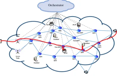
Fig. 1: Partially SDN and hybrid NFV mobile core Network of wireless networks
• NFs of the data plane are executed in the form of hybrid NFV. This way, some NFs are
executed on servers, and some of them are executed on physical function nodes.
This hybrid deployment can also model transition of the cellular networks from fourth-generation (4G) to 5G and 6G. Mainly because the transition budgets are limited, and only a part of the network can be upgraded at a time, especially for large-scale networks. In addition, as an emerging technology, SDN is not mature enough to replace the whole traditional net-work in a single step. Therefore, gradual software-defined and MCN implementation sounds inevitable to assess SDN feasibility in next generation of wireless networks. Evidently, the transition time is likely to extend over a several years span. During the transition, SDN should coexist with traditional networks [4]. In the partial SDN network, we can still implement centralized control of these SDN-enabled devices to save energy. However, the hybrid SDN is not as effective and flexible as in full SDN. Similarly, due to the implementation problems and costs, operators seem to be imperceptibly moving towards full NFV networks. Such arguments have led to works such as [5] and [7] to consider hybrid NFV architectures for 5G and 6G MCN.
In this paper, we consider a partial SDN and hybrid NFV network, as shown in Fig. 1 which can model different modes of combinations of SDN and NFV with traditional networking during this transition. In this network, we only consider the data plane where NFs are implemented as hybrid NFV (on servers or physical function nodes), and the transport network is partial SDN. We assume that an orchestrator performs all functions of control plane and control tasks related to NFV and SDN. The proposed system model is comprehensive for SDN/NFV networks where it can be deployed for full/partial SDN networks, full/hybrid NFV networks, or (partial) SDN/(hybrid) NFV networks.
propose an algorithm to save energy in the network. Based on the proposed algorithm, the unused nodes and links in the network are turned off to consume less energy. Our contributions are summarized as follows:
• This paper provides a framework to model the MCN of 5G during transition from 4G to
5G.
• The presented work is the first to address the problem of saving energy in partial SDN and
hybrid NFV MCN through the transition to 5G. Although energy efficiency, in traditional networks, SDN networks, and partial SDN networks is a well-studied problem, saving energy in partial SDN and hybrid NFV is a new problem that has not been addressed to the best of our knowledge.
• Energy efficiency in SDN/NFV networks is comprehensively modeled, including different
modes of SDN/NFV networks, e.g., (partial)SDN, (hybrid)NFV, partial SDN/hybrid NFV, partial SDN/full NFV, and full SDN/full NFV networks.
• The problem of energy efficiency in the considered network is formulated as a non-linear
integer programming (NLIP). The objective is to minimize the power consumption of the network components by turning off the unused or less-loaded components.
• Because of the NP-hardness of the resulting optimization problem, a suboptimal algorithm
based on the Viterbi Algorithm (VA) is proposed to solve the optimization problem. The algorithm starts via assigning weights to all nodes and links based on their on/off-states, as well as their energy consumption levels. The network is modeled as a multi-stage graph, and a candidate set determines the paths of flows, the type of NFs, and their locations to run for each flow. Ultimately, paths are selected based on a modified Djikstra’s routing algorithm (MDRA). We refer to this algorithm as modified Viterbi algorithm (MVA).
• Simulation results demonstrate that the performance of the network in terms of energy
efficiency, can be very close to optimum without a full migration to a SDN-NFV platform. The rest of the paper is organized as follows. Related work is presented in Section II. In Section III, the system model is described. In Section IV, the problem formulation of energy efficiency in partial SDN and hybrid NFV MCN for 5G is introduced. Subsequently, in Section V, an efficient algorithm based on MVA is proposed and its computational complexity are presented. In Section VI, the performance of our proposed algorithm is evaluated for different network sizes. Finally, Section VII concludes the paper.
II. RELATEDWORK
This paper sits in the intersection of three groups of works: research on the energy efficiency in SDN networks; the energy efficiency in the partial SDN networks and efficiency in the NFV. We will review these three of reserach trends and then we will highlight the novelties of this paper.
For full SDN networks, there exists a large body of works focusing on the energy efficiency either in data center networks, e.g., [8], [9], or on the conventional data networks. e.g., [10]. For the former cases, usually under-utilized data centers are switched off via SDN controllers [8], [9]. However, for the latter case, by considering the physical structure of switches, heuristic algorithms are proposed to reduce the energy consumption [11], [12]. None of these two cases is related to MCN and to fill this gap, we study the energy efficiency for the MCN armed by SDN and NFV for different scenarios of implementation e.g., partial SDN and hybrid NFV.
In [13], the problem of energy saving in partial SDN networks is addressed by switching off the SDN links and nodes.1 Those links and nodes are chosen through optimizing a novel
objective function using a heuristic algorithm. In [2], a partial SDN is deployed via a green abstraction layer which belongs to the European Telecommunications Standards Institute (ETSI) [15]. In this standard, multi energy-aware states are considered for the devices. In each state, the device consumes a certain amount of energy and attains a specific performance. An energy efficiency metric named Ratio for Energy Saving in SDN (RESDN) that quantifies energy efficiency based on link utility intervals is presented by [16]. A heuristics algorithm for maximize RESDN is presented.
NFV placement problems have received a lot of interest recently [17], [18]. [19]–[21] apply the Viterbi algorithm to solve their NFV resource allocation problems. In [20], [22] where NFVs are allocated to servers in the network to optimize objective functions, e.g., energy efficiency, subject to network limitations and required quality of services. These problems are inherently high dimensional and complex problems [23]. For instance, [22] deploys a Markov decision process to minimize energy consumption in NFV based networks. [19] has considered four types of costs for the problem of resource allocation in NFV, one of which is energy resources.
1
Partial SDN networks are first mathematically introduced in [14] where a fraction of switches are equipped with SDN capability..
[24] also uses migration to decrease energy consumption in the cloud data centers where it models the energy consumption of cloud network by considering the computing costs of the virtual elements on the physical servers, the migration cost for virtual elements across the servers, and the costs of transferring data between the virtual elements. In addition, it introduces a weight parameter to avoid excessive load of virtual element migrations. [25] designs a dynamic energy-saving model with NFV technology using an M/M/c queuing network with the minimum capacity policy where a certain amount of load is required to start the virtual machine, and an energy-cost optimization problem is formulated with capacity and delay as constraints. In [26], a new energy smart service function chain orchestrator is proposed in which NFV placement is adjusted to utilize more renewable energy in telecom-munication networks. A resource allocation problem, considering constraints on delay, link utilization, and server utilization, is presented in [27], which enables energy-aware SFC for SDN-based networks. In order to achieve the trade-off among energy saving, bandwidth usage minimization, and migration cost reduction, [28] proposes a VNF consolidation method (VCMM), which determines appropriate servers to be turned off by leveraging neural network with multiple characteristics of network status as input. VCMM migrates VNFs on servers to turn them off by adopting a greedy mechanism. In [6], an evolutionary architecture based NFV for 5G core is considered and an energy efficiency problem for data plane and control plane of the architecture is formulated. It also tests the proposed algorithm on a real-world testbed based on OpenStack and OpenDaylight. [29] addresses energy efficiency in NFV/SDN for internet of things networks where a new incentive mechanism exploratory works among energy suppliers and consumers is designed in order to encourage consumers to adjust their energy consumption based on available resources. In this paper, we propose a general system model which can be utilized for any type of full, partial, and non SDN/NFV networks. Saving energy in partial SDN and hybrid NFV MCNs is a new problem that has not been addressed to the best of our knowledge. The presented model and energy efficiency formulation for MCN networks can formulate the transition from 4G to 5G.
III. SYSTEMMODEL
We consider a partial SDN and hybrid NFV network, represented by an undirected graph
A ={N,E}, where N = {1,2,· · · , N} denotes the set of all nodes including SDN, NFV, and legacy nodes, and E = {1,2,· · · , E} denotes the set of E undirected links connecting the nodes. In this setup, we assume that a central orchestrator is responsible for providing coordination among all domain controllers, i.e., an SDN controller and the management layers
of the legacy nodes. Each mobile traffic flow is specified by its own rate limit and a specific set of NFs, which should be run on this flow in a specific order, called the service chain of this flow. In order to establish an end to end connection for this flow, a specific route to transfer data between the assigned nodes should be determined. In what follows, we provide a mathematical model to represent network limitations and flow characteristics.
A. Network Function Structure
In this setup, the set of all NFs are represented by G = {g1, g2,· · · , gK} where each service chain of a flow is a specific subset of G with predetermined order introduced by the orchestrator. All these NFs can be run in a virtualized manner, referred to VNFs in this case.
gk can be VNF k or implemented in a physical function node permanently as an NF. Whengk is a VNF, it requires a set of resourcesCgk ={c
1
k, c2k,· · · , cLk}whereclkrepresents the required resource of category l for VNFgk. In addition, the amount of ingress traffic rate that gk in a virtualized manner can process is rk. We refer to rk as a processing capacity of VNF gk [19].
B. Flow Representation
We assume that flow arrivals occur in a time-slotted manner, and the flows are received during a time-slot to be served at the beginning of the following time-slot. Consider a set of flows in a network asF. Each mobile traffic flowf can be represented asf = (sf, df, rf,Gf) where sf, df and rf denote the source, the destination, and the amount of incoming rate of flowf ∈ F, respectively. Here, we show a service chain of flowf asGf ={gf
1, g
f
2,· · · , g f
¯ Kf},
which is a set of NFs with a specific order to be run over flow f. K¯f denotes the number of NFs running over flow f, and g¯kf denotes k¯th NF that must be run for flow f. Note that
gkf¯ also belongs to G, however to show the order of NFs for each flow and their related
sequences, we use this notation per flow. The orchestrator has knowledge about which gk is related to g¯kf. In this paper, to denote the mapping of gk to gf¯k via Orchestrator, we use the
following notation
χfk→¯k(gk) =gkf¯ ∀gk∈ G, ∀gkf¯ ∈ Gf, ∀f,
where χfk→k¯(gk) represents the mapping stored in the orchestrator and utilized during the service time of flow f.
C. Nodes’ Categories and Features
In the mixed structure of traditional SDN and NFV-based networks in our setup, to run a service chain of any user’s request and provide the connections, there exist four sets of network nodes, i.e.,
• NT ={1,2,· · · , NT} as the set of traditional switches, called non-SDN nodes; • NS ={1,2,· · · , NS} as the set of SDN enabled switches, called SDN nodes;
• NN ={1,2,· · · , NN}as the set of NFV based servers running NFs in a virtualized manner and is referred to as NFV nodes;
• NM = {1,2,· · · , NM} as the set of physical function nodes, such as nodes of serving
gateways (SGW) and packet data network gateways (PGW) and is called non-NFV nodes. As a result, the total number of nodes in the network is NT +NS+NN +NM =N where each node u ∈ N has two states: 1) On-state in which u is on; and, 2) Off-state where u
is off. The orchestrator has access to the states of all nodes however, the state of SDN/NFV nodes, eg., N \NT can be dynamically adjusted. To represent states of the nodes, we define
α(u) as
α(u) =
0, if u∈ N \NT is in off-state,
1, otherwise.
To run a set Gf for each flow f ∈ F, orchestrator requires information about NFs that
each u ∈ NM ∪ NN can run, and the amount of capacity of each u ∈ NM ∪ NN. Each
non-NFV node u∈ NM can run a predetermined set of NFs. Let Gu ={gu1, gu2,· · · , guku}
represent the NFs which are run in node u∈ NM. Each nodeu∈ NM has limited capacity
of ingress rate denoted by ru.
Each NFV node u∈ NN can run all NFs in G, and has a limited capacity for L types of
required resources of NF. This limitation is denoted byCu ={c1u, c2u,· · · , cLu} whereclu is the maximum capacity of node u for type l of resources. At any instance, each node u ∈ NN
can just run one instance of VNF k. Specifically, if NF gk is run over u ∈ NN ∪ NM, we
define
µku =
1, if node u∈ NN ∪ NM runs gk, 0, otherwise.
To demonstrate that flow f is served by node u to run g¯k, we define
µ¯kfu =
1, if node u is selected to run g¯kf of flow f,
One practical point is that there exists a situation that more than two consecutive NFs are run in one node u ∈ NM for flow f. In this situation the incoming rate to non-NFV node
u∈ NM is equal to the rate of the first NF of flow f deployed on u∈ NM [30]. To consider
this point in our formulation, for all u∈ NM, we define the following variable
ζu¯kf =
0, if µkf¯
u µ ¯ k−1f
u = 1,
1, otherwise. D. Notations for Links and Paths
In our system model, (u, v)∈ E is a physical connection between two nodes u∈ N and
v ∈ N. Each node u ∈ NM ∪ NN only connects to a switch with a link, and the switch
connects to other switches with one or more links. For each link (u, v)∈ E, c(u, v) denotes its capacity. When u or v ∈ N \NT, link (u, v) is referred to as SDN link, and a set of all
SDN links is denoted by ES ⊆ E. In our setup, for each SDN link, orchestrator considers
two states: 1) On-state if link (u, v)∈ ES is on; 2) Off-state if (u, v)∈ ES is off. To denote
the on and off-states of link (u, v)∈ ES, we define
β(u, v) =
1, if (u, v)∈ ES is active,
0, otherwise.
Note that the orchestrator can control on-states and off-states of all SDN links.
When a physical connection between two nodes u and v does not exist, we consider a set of paths between two nodes denoted by Pu→v ={Pu1→v,Pu2→v,· · · ,PuJ→u→vv}, where Ju→v denotes number of all paths between nodes uand v. To mathematically represent which path
Pj
u→v is selected for the flow f, we define Γf ju→v =
1, ifPuj→vis selected for flow f between nodesu andv,
0, otherwise,
and, to show whether or not physical connection (u0, v0) belongs to path Pj
u→v, we define
ρju(→u0v,v0) =
1, if physical connection(u0, v0) belongs to Puj→v,
0, otherwise.
If two different nodes u and v run gf¯k and gk¯f+1, a path from Pu→v is selected for flow f. For the case that one node u∈ NM∪ NN are run gf¯k and g
f ¯
k+1, we denote a communication
E. Energy Model of Nodes and Links
When each nodeu∈ NT ∪ NS is in on-state, its consumed power is almost constant. Here,
we assume that this power is equal to a maximum consumed power of nodeu∈ NT∪NS, i.e.,
Pumax [13]. For NFV and non-NFV nodes, a linear model of power consumption is assumed for on-states [31]. For instance, when the ingress rate of node u∈ NN ∪ NM increases, the
consumed power increases accordingly. In this paper, we consider following expression for
power consumption of a node u∈ N \NT a(u)=
a(u) =
Pmax
u , u∈ NS is in on-state,
(θ+ (1−θ)rcu
ru)P
max
u , u∈ NN ∪ NM is in on-state,
0, u∈ N \NT is in off-state,
where Pumax is the maximum power consumed in node u and θ is a ratio of idle state power to full load power. An idle state represents the state that u is in on-state, however, there is no incoming flow for u. rc
u and ru denote the amount of current ingress traffic rate and maximum ingress traffic rate of the node u∈ NN ∪ NM, respectively.
Consumed power for link (u, v) ∈ E is constant in on-state [13]. When (u, v)∈ ES is in
off-state, its consumed power is equal to zero. Therefore, consumed power cost of link(u, v)
can be modeled as
a(u, v) =
Pmax
(u,v), (u, v)∈ E\ES or (u, v)∈ ES is in on-state, 0, otherwise.
From the above definitions, the presented system model has included different modes of SDN/NFV networks, e.g., traditional, (partial)SDN, (hybrid)NFV, partial SDN/hybrid NFV, partial SDN/full NFV, and full SDN/full NFV networks.
IV. PROBLEMFORMULATION
In this section, we introduce a problem formulation for energy-efficient resource allocation, where the objective is to minimize the number of active nodes and links. To state this formulation mathematically, we initiate our discussion by introducing practical constraints in our proposed model.
When a node u is in off-state, all physical connected links to this node should be in off-states, and vice versa. This constraint is represented as
C1: β(u, v)≤α(u), ∀u, v ∈ N,∀(u, v)∈ E,
C2: α(u)≤ X
{v|(u,v)∈E}
where C1 forces all links connected to node u to be in off-states if node u is in off-state, and C2 is utilized to turn off node u if all related links are in off-states.
To select node u for running an NF gkf¯ of flow f, the node must be able to execute the
NF. We can represent this condition as
C3: µkfu¯ ≤µku, ∀g¯kf ∈ Gf,∀u∈ N
M∪ NN,∀f.
Here, we assume that NF splitting is not allowed. Therefore, each NF of flow f must be run entirely in one node. Mathematically, this point can be represented as
C4: X
u∈NM∪NN
µkfu¯ = 1, ∀g¯kf ∈ Gf,∀f,
meaning that each gf¯k is only run in one node [17].
The sum of required capacities of type l of placed VNFs in node u should not exceed from the capacity of that node. We show this capacity limitation as
C5: K
X
k=1
µkuclk ≤α(u)clu, ∀l, ∀u∈ NN.
where right and left sides of inequality are the capacity of type l and the used capacity of type l of node u, respectively.
Another important point is when each flow f passes through some of NFs, e.g., tunneling and encryption, data rate of flowf will be changed due to additional overheads and signaling procedures in wireless networks [30]. Therefore, in this context for each gf¯k, it is assumed that there existsγ¯kf ≥0, such that when the incoming data rate of flowf togf¯k is equal torf, the outgoing rate of flow f from gf¯k is equal to γf¯krf. Thus, the ingress capacity limitation
of non-NFV node u∈ NM is defined as
C6: X
∀f
X
k∈Gf
ζukf¯ µ¯kfu rf
¯ k−1
Y
j=1
γjf ≤α(u)ru, ∀u∈ NM.
whererfQ¯k−1
j=1γ f
j is ingress rate of flow f for thek
th function. µ¯kf
u ensures that the function is executed at node u and ζ¯kf
u guarantees that the previous function is not executed at node
u. For nodes u ∈ NN, there is no need to check that the previous function is executed at
those nodes. Therefore, the ingress capacity limitation of VNF k placed in node u ∈ NN
can be expressed as
C7: X
∀f
µkfu¯ rf
¯ k−1
Y
j=1
cc(u, v) = X
∀f
X
gf¯k∈Gf
X
v0∈N
M∪NN,v06=u0
X
u0∈N
M∪NN
Ju0→v0
X
j=1
ρju(0u,v→v)0Γf ju0→v0µ ¯ kf v0ζ
¯ kf v0 rf
¯ k−1
Y
j=1
γ¯kf. (1)
After determining the places where all gkf¯ ∈ Gf in the network are run, one complete path between nodes should be assigned. To set this point, first, the sourcesf should be connected to the node u running g1f. This constraint can be represented as
C8:
Jsf→u
X
j=1
Γf jsf→u =µ 1f
u , ∀f,∀u∈ NM∪ NN. where µ1f
u denotes whether the first function of flow f is executed in node u or not. If it is executed, from the source to node u only one path is selected. Then, all other nodes running
gkf¯ ∈ Gf should be connected based on the order of gf ¯ k in G
f. This consecutive ordering of paths can be represented as
C9:
Ju→v
X
j=1
Γf ju→v =µ¯ku−1f.µ¯kfv , ∀f,∀u, v ∈ NM∪ NN,
meaning that only one path is selected between the nodes which run consecutive NFs. Finally, the destination should be connected to the node running the last NF (gf¯k) of flow f. This constraint is also represented as
C10:
Ju→df
X
j=1
Γf ju→df =µ ¯ Kf
u ∀f,∀u∈ NM∪ NN.
Consequently, from C8-C10, one complete path between the source and the destination of each flow is created. To provide reliable communication for different flows in the network, besides limitations on links capacity, we should consider an upper limit on link utilization to prevent unbounded queuing delay. The capacity used in link(u, v) is calculated in (1). Each link (u, v) is located in the path between two nodes u0 and v0, where they are executed at two successive functions of flow f , respectively. Thus, the ingress rate of node v0 is equal to the rate passed through link (u, v). In (1), ζv¯kf0 rf
Qk¯−1 j=1γ
f ¯
k calculates ingress rate of node
v0 which is equal to the rate of link (u, v). µvkf¯0 ensures that the kth function of flow f runs
in node v0. Γf ju0→v0 andρ
j(u0,v0)
u→v specify that the jth path is selected for u0 →v0 of flow f and link (u, v) is in jth path, respectively. Finally, to calculate the amount of capacity used by link (u, v), all functions and flows are added together.
In order to avoid congestion in the links, we consider a margin for the maximum links capacity and define 0 < τ(u, v) ≤ 1 as a utilization factor of link (u, v). Then, for link
min α(u),β(u,v),µk
u,µ
¯
kf u ,Γf ju→v
Z(α(u), β(u, v), µuk, µ¯kfu ,Γf ju→v)
subject to C1-C11
α(u), β(u, v), ζu¯kf, µku, µ¯kfu , ρ,u(→u,vv),Γf ju→v ∈ {0,1}.
(2)
C11: cc(u, v)≤τ(u, v)β(u, v)c(u, v), ∀(u, v)∈ E.
wherecc(u, v)denotes the used capacity of link(u, v)and must be less than the multiplication of the link capacity c(u, v), the link state β(u, v), and the link utilization τ(u, v).
To reach energy efficiency in the proposed framework, we define a new utility function as
Z(α(u), β(u, v), µuk, µ¯kfu ,Γf ju→v) = X u∈N \NT
a(u)α(u) + X (u,v)∈ES
a(u, v)β(u, v),
where the first term of the objective function shows the sum of the consumed power of all nodes except non-SDN nodes, i.e., u∈ N \NT, and, the second term represents the sum of
power consumed by all SDN links (u, v) ∈ ES. Given the above objective function and the
constraints from C1-C11, the problem of energy efficient optimization is formulated in (2). All variables of the optimization problem (2) are integers; thus, the problem is an integer programming. Several variables are multiplied together in C11, and so the optimization problem is non-linear. Therefore, the optimization problem belongs to the class of non-linear integer programming (NLIP) problems, which are known to be computationally complex. Even for simpler scenarios, for a large set of predefined paths, it is not trivial to solve the problem [32]. Consequently, proposing efficient algorithms with tractable computational complexity is essential. To reach this goal, we propose the Modified Viterbi Algorithm (MVA) to determine the place where all NFs are run and the routing between the nodes. In our proposed algorithm, instead of selecting one path for VA in each stage [33], we store Ψf¯k -tuple of paths in stage ¯k for some integer Ψf¯k. We will show that such modification can considerably increase the energy efficiency of this type of network. At the same time, the complexity of the algorithm remains polynomial in time. In Tables I and II, the parameters and the variables are summarized, respectively.
V. THEPROPOSEDALGORITHM
In this section, we introduce the steps of the proposed algorithm to solve the optimization problem. First, we present the weight assignment strategy based on the on and off-states and
TABLE I: Parameters
Symbol Description
N Set of nodes
NT Set of non-SDN switches
NS Set of SDN switches
NM Set of non-NFV nodes
NN Set of NFV enabled nodes
E Set of links ES Set of SDN links
Gf
Set of NFs Gf
Set of NFs of flowf
Gu Set of NFs ofu∈ NM
Cu Set of resources capacity of server nodeu
Ck Set of resources requirements of VNFk
Pu→v Set of all paths between nodesuandv
Pf∗ ˜
uf¯
k−1→u˜
f
¯
k
Path related to edge(˜uf¯k−1,u˜
f
¯
k) Πf¯k Set of selected nodes in stages f
¯
kfor flowf ˜
C Capacity matrix of a candidate path
¯
Kf Number of NFs for flowf a(u) Power cost ofu
Symbol Description
γ¯kf Data rising factor of NFg f
¯
k cl
u Resource capacity of typelof nodeu clk Resources requirements of typelVNFk ru Maximum ingress traffic flow of node u ∈
NN∪ NM
rk Maximum ingress traffic flow of VNFk Pumax Maximum consumed power of nodeu a(u, v) Power cost for(u, v)
c(u, v) Capacity of(u, v) τ Max link utilization
rf Traffic of flowf sf Source of flowf df Destination of flowf sf¯k Stagek¯of flowf
gf¯k k
th NF of flow f
ρj,u→(uv0,v0) To show if(u0, v0)exists inPuj→v wf(u) Weight ofu
wf(u, v) Weight of(u, v)
TABLE II: Variables Variable Description
Ψf¯k Number of stored paths in stages f
¯
k foru
α(u) Power state ofu β(u, v) Power state for(u, v)
µku To choose for nodeu∈ NN running VNFk µ¯kf
u To choose nodeu∈ NN running NFgkf¯
Γf,ju→v To select pathPuj→vfor nodesu,vfromPu→v
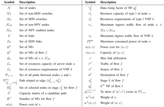
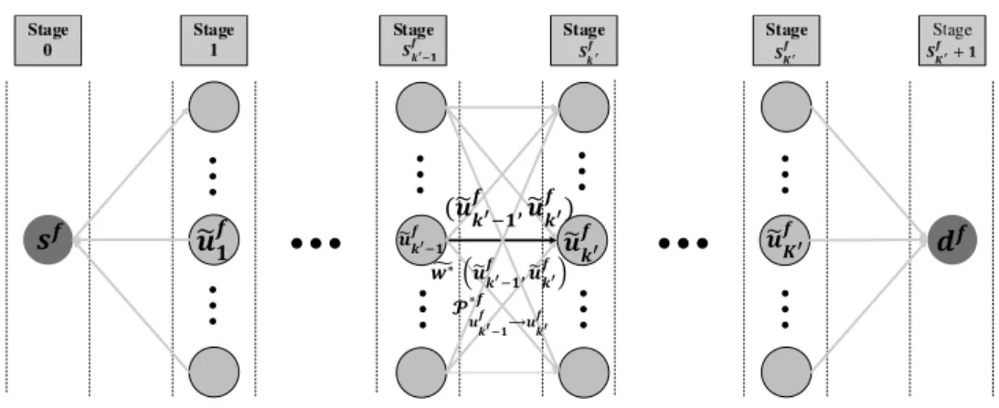
types of the nodes and the links. The weights are determined based on the energy consumption of the nodes or the links. If a node or a link is used, its weight is assigned by the amount of increased energy consumption of the network. The network is modeled by a multi-stage graph for each flow. The sets of candidate nodes for running NFs in each stage and paths between the stages are determined based on MVA. This algorithm is briefly demonstrated in Fig. 2 and Fig. 3 plots the flowchart of the algorithm. The algorithm is run for each flow. We assume that for the first flow, i.e., f = 1, all nodes and links are in off-states. The weight assignment strategy of all nodes and links is updated for each flow.
A. Weight Assignment Strategy
We consider the weight assignment of each node u∈ NS∪ NT for flow f as
wf(u) =
ε(u), if u∈ NT or u∈ NS is in on-state,
Pmax
u , if u∈ NS is in off-state,
where 0 < ε(u) 1, and ε(u) < a(u). Using this weight assignment strategy, we try to force the algorithm to utilize the resources of nodes u ∈ NS ∪ NT which are in on-state.
This is because for switches in our setup, we assume that the consumed power depends on the states (on/off) of a switch and it is not related to the load of the switch. Consequently, this weight assignment strategy tries to keep off-state nodes in the same states.
For the nodes running NFs, in addition to the difference between the power consumed in off-state and on-state, power consumption in on-state also depends on traffic load of that node. Accordingly, we define the following weight assignment strategy
wf(u) =
θPumax, if u∈ NN ∪ NM is in off-state,
(1−θ)rrf
uP
max
u , if u∈ NN ∪ NM is in on-state,
From practical considerations, we have θPmax
u (1−θ)r f ruP
max
u . Therefore, still via this strategy, we insist to keep the off-state nodes in those states.
Similarly, for each link (u, v), we consider the following weight assignment strategy
wf(u, v) =
ε(u, v), if(u, v)∈ E\ES or (u, v)∈ ES is in on-state,
a(u, v), if(u, v)∈ ES is in off-state,
where 0 < ε(u, v) 1, ε(u, v) a(u, v). Remarkably, since orchestrator cannot control the on-state and off-state of u∈ NT and (u, v)∈ E\ES, and since the configuration of these
nodes and links from off-state to on-state is time consuming, it is preferable to keep these nodes in on-states. Therefore, in our weight assignment strategies, the weights of these nodes and links are assigned to wf(u) =ε(u), wf(u, v) =ε(u, v), respectively.
B. Proposed Algorithm Based on Multi-Stage Graph Modeling
After the weight assignment strategy, for each flow f, a set of nodes running a set Gf should be determined. Then, the NFs and their related nodes should be connected through network paths based on the order of NFs in Gf, which are determined by the orchestrator. The placement of NFs and routing between nodes are two major interrelated tasks for our algorithm. To jointly perform these two tasks, we resort to the multi-stage graph model [19]. In our algorithm, a set of candidate nodes enabled to run gf¯k is the candidate set of stage
Fig. 2: Multi-stage graph modeling: for each nodes in two consecutive stages, MVA find edge(˜ufk¯−1,u˜
f
¯
k)with
weightw˜kf¯∗(˜u
f
¯
k−1,u˜
f
¯
k)andP f∗ ˜
uf¯
k−1→u˜
f
¯
k
.
¯
kf, as shown in Fig. 2. Let the stage of ¯kf to be denoted as sfk¯. We consider source and
destination as two predetermined stage ofsf0 andsfK¯+1, respectively. Therefore, a multi-stage
graph in our algorithm has K¯f + 2 stages. Between two consecutive stages, corresponding to two consecutive NFs in Gf, i.e., gf
¯ k and g
f ¯
k+1, there exists a set of edges related to paths
between candidate nodes of stages k¯f and k¯f + 1.
Note that this algorithm is executed for each flow f, and, between each node in stages ¯kf and each node in stagek¯f+1, only one edge is selected. This edge corresponds to the shortest path based on the weight assignment strategy from Dijkstra’s algorithm [34], discussed in Section V-C.
1) Candidate Set Selection: For each g¯kf ∈ Gf, the candidate set should be chosen based on the capability of nodes to run gkf¯ and their capacities. In the initial phase of our proposed
algorithm, for each flow f, we should update the capacity of nodes and links based on the place where running NFs and routing of flows 1 to f −1. In the followings formulas, we show how this update can be performed from C5, C6, and C7. First to verify which node
u∈ NN is capable to run g¯kf in terms of available capacity, we consider ˜
clfu =α(u)clu−
K
X
k=1
µkuclk, ∀l, ∀u∈ NN,
which shows the updated capacity limit of node u ∈ NN for type l resource of flow f.
Therefore, to verify if node u∈ NN can run NF g¯kf, the following modified constraint of C5
can be applied
˜
Cf5:clk≤c˜,fu ∀l, ∀u∈ NN.
Start
Select Candidate
nodes
Find edge from
candidate nodes
Store paths for
candidate nodes
If the last node
is the source
node
Update weights
Go to next
stage
NO
Yes
Weight
Assignment
End
Select path
with minimum
weight
Parameters
of flow f
˜
rfu =α(u)ru− f−1
X
f=1
X
k∈Gf
ζu¯kfµkfu¯ rf
¯ k−1
Y
j=1
γjf, ∀u∈ NM.
Therefore, to verify if nodeu∈ NMhas appropriate ingress capacity for flowf, following
modified version of C6 is applied
˜
Cf6: X k∈Gf
ζu¯kfµkfu¯ rf
¯ k−1
Y
j=1
γjf ≤r˜uf, ∀u∈ NM.
Also, the updated ingress capacity of VNF k placed in node u∈ NN can be expressed as
˜
rkuf¯ =rk− f−1
X
f=1
µ¯kfu rf
¯ k−1
Y
j=1
γjf, χfk→k¯(gk) =gf¯k,
and, the modified ingress capacity limitation of VNF k placed in node u based on C7 can be examined by
˜
Cf7: X k∈Gf
ζukf¯ µ¯kfu rf
¯ k−1
Y
j=1
γjf ≤r˜¯kuf , ∀u∈ NM.
In our algorithm, for each flow f, we will verify C˜f5-C˜f7 to derive the candidate set of stage k¯f which is denoted by Πfk¯.
2) Path Selection: After selecting nodes for all stages, the paths between nodes in any two consecutive stages should be determined in order to build the end to end connection between source and destination of flowf. First, in order to find these paths, we must update the capacity limitation of all links (u, v) in the network based on the traffic flow of f = 1,· · · , f−1, which is defined as
˜
cf(u, v) =τ(u, v)β(u, v)c(u, v)− f−1 X
f=1 X
gf¯k∈Gf
X
v0∈NM∪NN,v06=u0
X
u0∈N
M∪NN
Ju0→v0
X
j=1
ρju(0u,v→v)0Γ f j u0→v0µ
¯ kf v0ζ
¯ kf v0r
f ¯ k−1 Y
j=1 γf¯k,
wherec˜f(u, v)is the utilized capacity of link (u, v)by flows f = 1,· · · , f−1. Therefore, C11 can be modified as
˜
Cf11: X
gf¯
k∈G
f
X
v0∈N
M∪NN,v06=u0
X
u0∈N
M∪NN
Ju0→v0
X
j=1
ρju(0u,v→v)0Γ
f j u0→v0µ
¯ kf v0ζ
¯ kf v0 rf
¯ k−1
Y
j=1
γ¯kf ≤˜c f
(u, v), ∀(u, v)∈ E.
Our objective is to minimize the energy consumption of the network. So, next, we need to propose an algorithm to find a path with the least weight, based on the energy consumption of nodes and paths. To reach this goal, we develop a Modified Viterbi Algorithm (MVA) in which an MDRA is applied to find only one path between nodes of each two consecutive stages. Our proposed MDRA will be explained in Section V-C.
For two consecutive stages sf¯k−1 and s f ¯
k, we obtain edge (˜u f ¯ k−1,u˜
f ¯
k) for u˜ f ¯
k−1 ∈ Π f ¯ k−1, ˜
uf¯k ∈Π f ¯
k based on our proposed algorithm in Section V-C, where its output is w˜ f ¯ k(˜u
f ¯ k−1,u˜
f ¯ k) defined as a weight of a path Pf
˜ uf¯
k−1→u˜
f
¯
k
for edge (˜ufk¯−1,u˜ f ¯ k). In stage sfk¯, MVA intends to choose a number ofψ
f ¯
k paths from s d
to u˜f¯k with the smallest
weights, ∀u˜f¯k ∈ Π f ¯
k. To do so, for each node u˜ f ¯
k−1 ∈ Π f ¯
k−1 and each node u˜ f ¯ k ∈ Π
f ¯
k, MVA
considers the edge(˜uf¯k−1,u˜ f ¯
k). Consequently, the candidate paths leading tou˜ f ¯
k are the union of the ones stored in each of nodesu˜fk¯−1∈Π
f ¯
k−1extended byP f ˜ uf¯
k−1→u˜
f
¯
k
, with their corresponding weights computed as the summation of the weights of the two distinct parts of the path, i.e.,
˜
wf¯k(˜u f ¯ k−1,u˜
f ¯
k) added to the weight of the path stored in u˜ f ¯
k−1. Then, the paths eligible to be
stored in nodeu˜f¯k are theψ f ¯
k paths with the smallest weights chosen from the aforementioned paths.
As mentioned before there is a chance to select a specific nodeu∈ NN more than once to
place more than two VNFs for flow f. In this case, we need to update the capacity limitation of each specific node u∈ NN for each selected path of flow f based on the above explained
procedure. To address this issue in our algorithm, we define a matrix C˜ = [˜˜clf
u]NN×L, where ˜
˜
clf
u is the updated capacity limit of the resource type l of node u ∈ NN for flow f. This
matrix, along with the path’s corresponding weight, is stored in node u˜fk¯. At stage zero, the
entries of the matrix are initialized as c˜˜lf
u = ˜clfu. To meet the constraint on the capacity limit of node u˜f¯k, in stage s
f ¯
k, the paths satisfying the following constraint remain in the set of candidate paths of node u˜fk¯, and are evicted otherwise:
˜ ˜
C5: clk ≤˜˜clfu, ∀l.
In addition, when a path meets the above constraint, ˜˜clf
u should be updated as ˜
˜
clfu = ˜˜clfu −clk, ∀l.
For stage sfK¯+1, we have ψ f
¯
K+1 paths from source to destination. The path with minimum
weight, corresponding to the least energy consumption is selected. The above MVA is summarized in Algorithm 1.
Finally, the output factors of Algorithm 1 are the selected path between source and destination Pf
as well as variables α(u), β(u, v), µk u, µ
¯ k,f
u and Γ
f,j u→v. w
f(u)
, wf(u, v) , a(u),
a(u, v). Afterwards, all capacities are updated according to values of Algorithm 1. C. Modified Dijkstra’s Routing Algorithm
In this section, we explain our proposed MDRA to find an edge between u˜f¯k−1 and u˜ f ¯ k of two consecutive stagessfk¯−1 and s
f ¯
k. Here, we have a set of the pathsPu˜f¯ k−1→u˜
f
¯
k
Algorithm 1: Modified Viterbi Algorithm (MVA) Input:A,G,Gu,Cgk,Cu,f = (s
f, df, rf,Gf),wf(u), wf(u, v), c(u, v), c˜f(u, v), β(u, v),a(u, v)
∀(u, v)∈ E,α(u), a(u), µku, , µ
¯
kf
u , ru, ˜ruf, rk, r˜ f
¯
ku, ˜c lf
u,∀u∈ N, ∀k
Output: A path fromsf todf,α(u),β(u, v),µku,µ
¯
k,f
u andΓf,ju→v
forsf¯k=1:K¯ do for∀u∈ NM do
if(C˜f6 holds) & (gf¯k ∈ Gu)then
Addu toΠf¯k;
Find edge (˜uf¯k−1, u)and its weight with MDRA∀u˜
f
¯
k−1∈Π
f
¯
k−1;
Storeψf¯k paths with least weights from a set of candidate paths;
end end
for∀u∈ NN do
if(µ¯kfu = 1) & (C˜
f
7 holds)then
Addu toΠf¯k; Find edge (˜uf¯k
−1, u)and its weight with MDRA∀u˜
f
¯
k−1∈Π
f
¯
k−1;
Storeψf¯k paths with least weights from a set of candidate paths;
end if(µ¯kf
u = 0) & (C˜
f
5 holds)then
Addu toΠf¯k;
Find edge (˜uf¯k−1, u)and its weight with MDRA∀u˜
f
¯
k−1∈Π
f
¯
k−1;
forAll candidate paths do
forl=1:Ldo
if C˜˜f5 does not holdthen
Remove this path from set of candidate paths;
end end end
Storeψf¯k paths with least weights from candidate paths;
Update C˜ of stored paths;
end end end
Find edge(˜uf¯k, df)with MDRA∀u˜ f
¯
k−1∈Π
f
¯
k;
Find weights of candidate paths todf;
Select a path with smallest weight;
Return Pf and variables α(u),β(u, v),µk u,µ
¯
k,f
u andΓf,ju→v;
S D 3 4 1 2 {a} {a,b} {c,d}
{c, (b or d)}
{(b, c) or (b, d) or (c, d)} 10
6
5
(a) The topology of the network
S 1 3 1 4 5 4 5 2 4 5 2 D Stage 1 (Function a) Stage 2 (Function b) Stage 3 (Function c) Stage 4 (Function d) Stage 0 (Source) Stage 5 (Destination) Weight=11 Weight=9 Weight=17 Weight=18
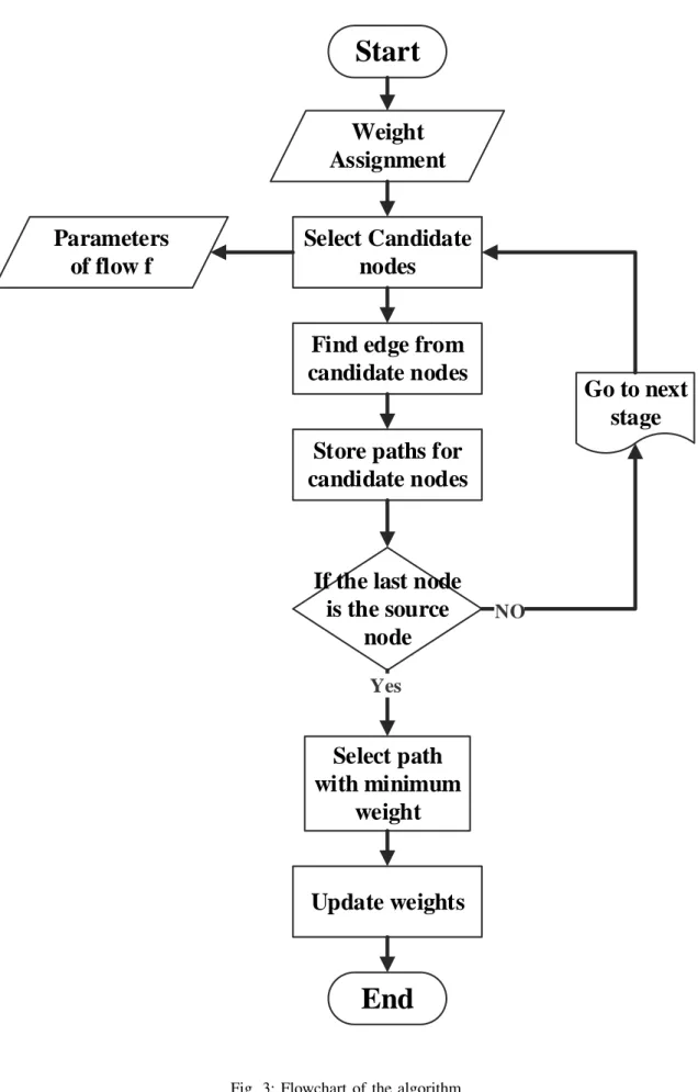
(b) The stages, the candidate nodes and the routes Fig. 4: An illustrative example of proposed algorithm
to choose a path with minimum weight corresponding to minimum power consumption of nodes and links. We resort to Dijkstra’s algorithm [34]. However to consider the capacity limitation of links and the weights of nodes, we propose a modified Dijkstra’s algorithm to find a path in graph A(N,E) for nodes u˜fk¯−1 and u˜
f ¯
k. In our proposed MDRA, we update
weight of each link as
˜
w¯kf(u, v) =
wf(u, v) +wf(u) +wf(v), if C˜f11 holds,
∞, Otherwise,
where if there is no capacity, the weight of that link is set to infinity, meaning that this link will be avoided to choose for flowf2. In addition, the nodes’ weights are considered in routing
via summation of nodes’ weights to their corresponding weights of physical connected links. In this paper, similar to [17], [35], we develop Dijkstra’s algorithm. Consequently, MDRA chooses the shortest path based on Dijkstra’s algorithm denoted byPf∗
˜ uf¯
k−1→˜u
f
¯
k
. Another output of MDRA is w˜¯kf∗(˜u
f ¯ k−1,u˜
f ¯
k) corresponding to the weight of P f∗
˜ uf¯
k−1→˜u
f
¯
k
.
D. Illustrative Example
In this section, we present an example of the proposed algorithm for the network of Fig. 4, and also show why we should store more than one path for the nodes. As it can be seen in Fig. 4, nodes 1 and 2 are non-NFV which run NFs of {a, b} and {c, d}, respectively. Node 3 runs NF {a} and cannot run other NFs. NF {c} is run on node 4 and it can be placed one of two NFs {b} and {d}. Node 5 can execute two NFs out of{b}, {c}, and {d}. In this network, the weights of the paths are as shown in Fig. 4.
Consider a flow f = {S,D,100 Mbps,Gf}, where ”S” and ”D” denote the source and the destination of flow f, respectively, and Gf ={a, b, c, d}. At each stage of the proposed algorithm, the nodes which can execute that NF are selected as noted in Fig. 4 (a). For 2In Dijkstra’s algorithm, the links only have weights and weights of nodes does not considered. In addition, in Dijkstra’s
algorithm, the capacity of nodes are not considered while in our proposed algorithm, we consider the capacity of nodes as well [34].
example, in stage one, nodes 1 and 3 are selected, and in stage two, nodes 1, 4, and 3 are chosen. Let us assume that for each stage up to 3 paths can be stored.
For each candidate node in stage sf¯k, its edges to all other nodes in the previous stage are
found. Note that for each edge, there exists one path, including one physical link or several connected physical links. For instance, for edge (1,4) between the second and third stages, its corresponding path 1 → 4 includes one physical link. Likewise, for edge (1,5) again between the second and third stages, its corresponding path is 1 → 4 → 5 including two physical links (1,4) and (4,5). After verifying C5,˜˜ ψkf¯ ≤ 3, k¯ = 1,2,3, the paths with the
lowest weights from the source to that node are stored. For example, for node 4 in the third
stage, path S →3→4→4 with weight 9, path S →1→1→4 with weight 11, and path
S →1→4→4 with weight 11 are stored.
Consider the case that ψf¯k = 1, k¯ = 1,2,3, then the red path is selected for candidate
node 4 in the third stage. Consequently, in the fourth stage, again, the red path is stored to run function d. Finally, the red path from the source to the destination with weight 18 is selected for the flow f. However, when ψkf¯ ≤3, k¯= 1,2,3, the red and the green paths are
stored for candidate node 4 in the fourth stage. Finally, the green path from the source to the destination with weight 17 is selected, which has a lower weight than the red path. This illustrative example shows how with MVA and considering three candidate paths instead of one path in VA, the performance of the network can be improved in terms of energy efficiency.
E. Computational Complexity
In this section, we investigate the computational complexity of the proposed algorithms and compare them with the exhaustive search. At each stage of the proposed algorithm,
NM +NN nodes are verified, and for each node, O(NM +NN) edges are found. For each candidate node in each stage, all links (the number of links is E) are first verified, and then, Dijkstra’s algorithm runs with complexity O(E+Nlog(N)) [36]. Thus, MDRA performs
O(E +Nlog(N) + E) = O(2E +Nlog(N)) computations. The number of stages in the algorithm is |Gf|. Therefore, the computational complexity of Algorithm is O(|Gf|(N
M +
NN)2(2E+Nlog(N))), which is polynomial time.
However, the computational complexity of the exhaustive search algorithm for optimization problem (2) is O(e(N−2)!×2(NS+NN)×2E×2|Gf|(NM+NN)), wheree is Neper number. The
first term, i.e., e(N −2)!, approximates the entire paths which should be searched for the fully connected graph between two specific nodes. The second term, i.e., 2(NS+NN), is the
number of all on/off states of SDN and NFV nodes that should be searched via exhaustive search. 2E denotes the number of the entire on/off states of SDN links. Finally, to find out which node runs a specific NF, exhaustive search algorithm should search among2|Gf|(NM+NN)
possible scenarios among nodes. Comparing the exponential order of the exhaustive search with polynomial order of Algorithm 1 demonstrates its efficiency in terms of computational complexity.
VI. SIMULATIONS
In this section, we evaluate the performance of MVA versus different network parameters and scenarios. We first compare the performance of MVA with the optimal solution in a small network with normalized parameters. Then, we evaluate the performance of MVA in three different sizes of MCNs.
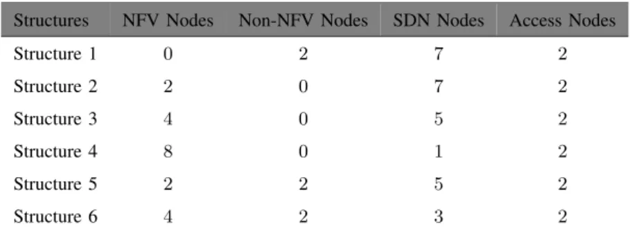
To compare MVA and the optimal solutions, we consider a connected network with 11 nodes and 19 links. We assume that all switches are SDN. For the nodes that execute the functions, six structures are considered, whose details are shown in Table III. The properties of the nodes, links, and functions are shown in Table IV. For NFV nodes, a resource type is considered, and the capacity of this type of resource is shown in this table. In rows 8 and 9, three numbers are related to NFV node type 1, NFV node type 2, and NFV node type 3, respectively. Two access nodes are considered in the network. We assume that the traffic of access nodes varies from 1 to 5. Figure 5 shows the solution of the proposed algorithm and the optimal solution (exhaustive search) for different network structures. The figure demonstrates that the proposed algorithm, in most cases, achieves the optimal solution and, in other cases a near-optimal solution. When there are only NFV nodes or non-NFV (structures 1 to 4), the algorithm obtains the optimal solution. In hybrid NFV structures (structures 5 and 6), the algorithm deviates slightly from the optimal response by increasing the rate of access nodes. However, in the worst case, the proposed algorithm has a response time of 1.1 times the optimal response. in low- and medium-load cases, the use of NFV nodes always reduces network energy. Conversely, in high-load cases, the consumed energy of the network is not much different from the case where NFV and non-NFV nodes are used.
Three MCNs are based on LTE coverage map in [37]: 1) a small-sized network which
can be used for Poland, 2)a medium-sized network which can be deployed to model regions like Iran, and 3) a large-sized network which is according to the USA network model. The parameters of these networks are displayed in Table V. The number of nodes in the networks
Structures NFV Nodes Non-NFV Nodes SDN Nodes Access Nodes
Structure 1 0 2 7 2
Structure 2 2 0 7 2
Structure 3 4 0 5 2
Structure 4 8 0 1 2
Structure 5 2 2 5 2
Structure 6 4 2 3 2
TABLE IV: Characteristics of Nodes, Links and Functions
Parameters NFV Node type 1 (Structure 2 and 5)NFV Node type 2 (Structure 3 and 6)NFV Node type 3 (Structure 4)Non-NFV Nodes Switches Links
Idle Power 50 25 12.5 50 10 5
Peak Power 50 25 12.5 50 0 0
Ingress Capacity 10 5 2.5 10 - 5
Resources 60 30 15 - -
-Functions 1−5 1−5 1−5 1−3or4−5 -
-Parameter VNF 1 VNF 2 VNF 3 VNF 4 VNF 5
Resource Required 20or10or5 20or10or5 20or10or5 30or15or7.5 30or15or7.5
Ingress Capacity 10or5or2.5 10or5or2.5 10or5or2.5 10 or 5 or 2.510or5or2.5 10or5or2.5
and the data rates of flows are based on [32]. In this table, the access nodes generate traffic flows.
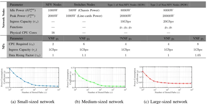
The characteristics of the network nodes and NFs are shown in Table VI. The types of switches are in accordance with the setup in [19]. The traffic rate for each flow is a random variable uniformly chosen between 1Mbps and 900Mbps, and we consider a set of NFs as G = {g1, g2, g3, g4, g5}. Assume there exist two types of non-NFV nodes: 1) SGW
Gu1 ={g1, g2, g3}and, 2) PGWGu2 ={g4, g5}. We suppose that all NFs must be executed for
all flows, i.e., G =Gf for all f. Since there exists no related work to this paper, we compare our results with the case that only one path is stored in each stage, i.e., the traditional VA.
In all simulation scenarios, the consumed power in our algorithm is compared to the result of the case where all network components are active. When the number of network
com-1 2 3 4 5
Rate of Access Nodes 0 100 200 300 400 Power Consumption Optimal MVA
(a) Structure 1
1 2 3 4 5
Rate of Access nodes 0 100 200 300 400 Power Consumption Optimal MVA
(b) Structure 2
1 2 3 4 5
Rate of Access nodes 0 100 200 300 400 Power Consumption Optimal MVA
(c) Structure 3
1 2 3 4 5
Rate of Access nodes 0 100 200 300 400 Power Consumption Optimal MVA
(d) Structure 4
1 2 3 4 5
Rate of Access nodes 0 100 200 300 400 Power Consumption Optimal MVA
(e) Structure 5
1 2 3 4 5
Rate of Access Nodes 0 100 200 300 400 500 Power Consumption Optimal MVA
(f) Structure 6 Fig. 5: Rate of Access Nodes versus power consumption for Optimal Solution and MVA
η= Consumed power of network using MVA
Consumed power of reference network while all its network components are active (3)
TABLE V: Parameters of three scenarios
Parameters Small-Sized Network Medium-Sized Network Large-Sized Network
Number of Access Nodes 16 60 100
Number of Switches 32 90 150
Number of Links 88 282 460
Number of Backbone Links 4 42 60
Number of Type 1 of Non-NFV Nodes (SGW) 4 6 10
Number of Type 2 of Non-NFV Nodes (PGW) 2 3 5
Number of NFV Nodes 8 12 25
Number of Internet Exchange Points (IxP) 1 3 5
Capacity of links [1M bps,1Gbps] [1M bps,1Gbps] [1M bps,1Gbps]
Capacity of backbone links 40Gbps 40Gbps 40Gbps
Data rate of flow of access nodes [1M bps,900M bps] [1M bps,900M bps] [1M bps,900M bps]
ponents increases or decreases, the consumed power is compared to the reference networks, e.g., the networks in Table V. Therefore, we define the power consumption coefficient as (3). One of the important parameters to improve the performance of the proposed MVA is the number of stored paths, i.e.,ψf¯k. To show the effect of this parameter, we evaluate the amount
of power consumed versus ψkf¯. We also consider ψ =ψ f ¯
k, ∀k,¯ ∀f and that all switches are SDN. In Fig. 6, the number of stored paths (ψ) versus the power consumption coefficient (η) is demonstrated for three network scenarios. As expected, it reveals from Fig. 6 that storing more paths for each node leads a better energy efficiency in the networks. In small-sized,
TABLE VI: The characteristics of the network nodes and network functions
Netw
ork
Nodes
Parameter NFV Nodes Switches Nodes Type 1 of Non-NFV Nodes (SGW) Type 2 of Non-NFV Nodes (PGW)
Idle Power (θPmax
u ) 1000W 500W (Chassis Power) 8000W 8000W
Peak Power (Pmax
u ) 2000W 1000W (Line-cards Power) 20000W 20000W
Ingress Capacity (ru) — — 10Gbps 20Gbps
Functions — — g1, g2, g3 g4, g5
Physical CPU Cores 16 — — —
NFs
Parameter VNFg1 VNFg2 ?VNFg3 VNFg4 VNFg5
CPU Required (ck) 2 6 4 4 8
Ingress Capacity (rj) 1Gbps 1Gbps 1Gbps 1Gbps 1Gbps
Data Rising Factor (γk) 1 1.1 1 1 1.05
100 101 102 103 104
Number of Stored Paths ( ) 0.52
0.54 0.56 0.58 0.6
Power Consumption
Coefficient (
)
(a) Small-sized network
100 101 102 103 104
Number of Stored Paths ( ) 0.6
0.65 0.7 0.75
Power Consumption Coefficient (
)
(b) Medium-sized network
100 101 102 103 104
Number of Stored Paths ( ) 0.6
0.65 0.7 0.75 0.8
Power Consumption Coefficient (
)
(c) Large-sized network Fig. 6: Number of stored paths (ψ) versus the power consumption coefficient (η)
0 200 400 600 800 1000 1200
Average Rate of Access Nodes (Mbps)
0.2 0.4 0.6
Power Consumption
Coefficient (
)
(a) Small-sized network
0 200 400 600 800 1000 1200
Average Rate of Access Nodes (Mbps)
0.4 0.6 0.8
Power Consumption
Coefficient (
)
(b) Medium-sized network
0 200 400 600 800 1000 1200
Average Rate of Access Nodes (Mbps)
0.2 0.4 0.6 0.8
Power Consumption Coefficient (
)
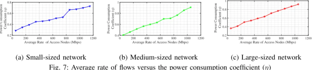
(c) Large-sized network Fig. 7: Average rate of flows versus the power consumption coefficient (η)
medium-sized, and large-sized networks, if 64, 128, and 128 paths are stored for each node, the consumed power decrements about 8%, 10%, and 12%, respectively. From Fig. 6 when
ψ = 1024, the performance of our algorithm approaches the case that all paths are stored in
the three network scenarios.
Fig. 7 plots the percentage of the consumed power in the three network scenarios versus the average data rate of the access nodes, i.e.,rf. For this simulation, we assume all switches are SDN. Fig. 7 (a) shows that for the small-sized network, by increasing the average data rate of the access nodes from 50Mbps to 1150Mbps, the consumed power of the network rises from 30% to 75%. Figures 7 (b) and 7 (c) show that in the medium-sized and large-sized networks by increasing the average data rate of access nodes, the consumed power of networks rises approximately from 40% to 90%. These results verify that increasingrf leads to an increment of the consumed power as expected.
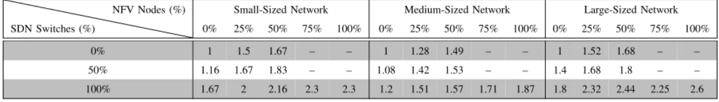
Now we aim to evaluate the effect of transition from the non-SDN and non-NFV network to the full SDN and full NFV networks in terms of energy efficiency. To answer this critical issue, in Figs. 8-10, for different numbers of NFV nodes and non-NFV nodes and for different percentages of SDN switches, the power consumption coefficient of the three network scenarios are plotted versus the data rate of access nodes. In Fig. 8, all switches belong to SDN nodes. In Fig. 9, 50% of switches belong to SDN nodes, and in Fig. 10, all switches are non-SDN. For these figures, the average data rate of the access nodes are 100Mbps, 300Mbps, 500Mbps, 700Mbps, and 900Mbps.
Figure 8 (a) show that by increasing the number of NFV nodes in the small-sized network where all switches of networks are SDN, the consumed power of the network decreases. When there are 20 NFV nodes in the network, the network consumes between 8% and 20% less power than the case that there does not exist any NFV node in the network. Figure 8 (b) shows that in the medium-sized networks and in the case that there are only NFV nodes in the network, the network consumes about 20% less power than in a network without NFV nodes. In the large-sized network scenario, Fig. 8 (c) shows that by increasing the number
of NFV nodes from zero to 90%, η reduces by up to 50%.
100 300 500 700 900
Average Rate of Access Node (Mbps)
0 0.2 0.4 0.6 0.8
Power Consumption Coefficient (
)
8 NFV Nodes 4 SGWs 2 PGWs 4 NFV Nodes 4 SGWs 2 PGWs 0 NFV Nodes 4 SGWs 2 PGWs
(a) Small-sized network
100 300 500 700 900
Average Rate of Access Node (Mbps) 0
0.5
Power Consumption Coefficient (
6 NFV Nodes 4 SGWs 2 PGWs 0 NFV Nodes 4 SGWs 2 PGWs
(b) Medium-sized network
1 2 3 4 5
Average Rate of Access Nodes (Mbps)
0 0.5
Power Consumption
Coefficient (
25 NFV Nodes 10 SGW 5 PGW 13 NFV Nodes 10 SGW 5 PGW 0 NFV Nodes 10 SGW 5 PGW
(c) Large-sized network Fig. 8: Number of NFV nodes and non-NFV nodes versus the power consumption coefficient (η) for 100% SDN switches
100 300 500 700 900 Average Rate of Access Node (Mbps) 0
0.5 1
Power Consumption Coefficient (
) 8 NFV Nodes 4 SGWs 2 PGWs4 NFV Nodes 4 SGWs 2 PGWs 0 NFV Nodes 4 SGWs 2 PGWs
(a) Small-sized network
100 300 500 700 900
Average Rate of Access Nodes (Mbps) 0
0.5 1
Power Consumption Coefficient (
) 12 NFV Nodes 6 SGWs 3 PGWs6 NFV Nodes 6 SGWs 3 PGWs
0 NFV Nodes 6 SGWs 3 PGWs
(b) Medium-sized network
100 300 500 700 900
Average Rate of Access Nodes (Mbps)
0 0.2 0.4 0.6 0.8 1 Power Consumption Coefficient ( )
25 NFV Nodes 10 SGWs 5 PGWs 13 NFV Nodes 10 SGWs 5 PGWs 0 NFV Nodes 10 SGWs 5 PGWs
(c) Large-sized network Fig. 9: Number of NFV nodes and non-NFV nodes versus the power consumption coefficient (η) for 50% SDN switches
for the three network scenarios, all nodes are in on state for a certain amount of traffic in the network. For example, in the small network scenario in Fig. 7 (a), when the data rate is greater than 500Mbps, all nodes are in the on state. As a result, the consumed power exponentially increases. As concluded from Fig. 8, in the case that there is no NFV node, when the average data rate increases from 500Mbps to 700Mbps, the consumed powers of the three network scenarios rise significantly. However, for the hybrid NFV networks, the consumed power will gradually increase by increasing the data rates of access nodes in the network. For the same data rate, with increasing the number of NFV nodes in all three network scenarios, the amount of consumed power decreases.
The same behavior can be observed in Figs. 9 and 10 for the case that 50% and 0% of switches are SDN, respectively, i.e., by increasing the number of NFV nodes in the networks, energy consumption has been reduced. In addition, when there is no NFV node in the networks, by increasing data rates of the access nodes from 500Mbps to 700Mbps, the power consumption coefficient (η) significantly increases. According to Figs. 8, 9, and 10, the more number of SDN nodes in the network, the more energy will be saved by increasing the number of the NFV nodes. Similarly, if traffic data rates of the access nodes are low, by increasing the number of NFV nodes, we can save more energy in the network.
According to Figs. 8, 9, and 10, in most cases, the power consumption coefficientη, of the networks with hybrid NFV nodes approach the power of networks with full NFV nodes. For instance, in Fig. 8 (a), η for a network with 20 NFV nodes is close to η for a network with 11 NFV nodes. According to the migration cost of swapping non-NFV/non-SDN nodes to NFV/SDN node, with the hybrid NFV scenarios, mobile operators can approximately achieve