Vol 6, No 6 (2015)

(1)

Available online throug

ISSN 2229 – 5046

International Journal of Mathematical Archive- 6(6), June – 2015 84

NUMERICAL SOLUTION OF FUZZY DIFFERENTIAL EQUATIONS

BY USING MODIFIED FUZZY NEURAL NETWORK

EMAN A. HUSSIAN*

Asst. Prof., Dep. of Mathematics. College of Sciences.

Al-Mustansiriyah University, Baghdad, Iraq.

MAZIN H. SUHHIEM

Asst. Lec., Dep. of statistics,

College of Adm. and Econ. University of sumar, Baghdad, Iraq.

(Received On: 31-05-15; Revised & Accepted On: 22-06-15)

ABSTRACT

I

n this paper, we introduce a hybrid approach based on modified fuzzy neural network and optimization teqnique to

solve fuzzy differential equations. Using modified fuzzy neural network makes that training points should be selected over an open interval without training the network in the range of first and end points. Therefore, the calculating volume involving computational error is reduced. In fact, the training points depending on the distance selected for training neural network are converted to similar points in the open interval by using a new approach, then the network is trained in these similar areas. In comparison with existing similar neural networks proposed model provides solutions with high accuracy. The proposed method is illustrated by four numerical examples.

Keywords: Fuzzy differential equation, Modified fuzzy neural network, Feedforward neural network, BFGS method,

Hyperbolic tangent function.

1. INTRODUCTION

Nowadays, fuzzy differential equations are a popular topic studied by many researchers since it is utilized widely for the purpose of modeling problems in science and engineering. Most of the practical problems require the solution of a fuzzy differential equation which satisfies fuzzy initial or boundary conditions. The theory of fuzzy differential equations was treated by Buckley and Feuring [9], Kaleva [16,17], Nieto [28], Ouyang and Wu [32], Seikkala also recently there appeared the papers of Bede, Bede and Gal [8], Diamond [10,11], Georgion et al., [14] Nieto and Rodriguez-Lopez [29]. In the following, we have mentioned some numerical solutions which have proposed by other scientists. Abbasbandy and Allahviranloo have solved fuzzy differential equations by Runge-Kuta and Taylor methods [1, 2]. Also, Allahviranloo et al. solved differential equations by predictor- corrector and transformation methods [3, 4, 5]. Ghazanfari and Shakerami developed Runge-Kuta like formula of order 4 for solving fuzzy differential equations [13]. Nystrom method has been introduced for solving fuzzy differential equations [18].

In 1990 Lee and Kang [19] used parallel processor computers to solve a first order differential equations with Hopfield neural network models. Meade, Fernandes and Malek [22, 27] solved linear and nonlinear ordinary differential equations using feed-forward neural network architecture and 𝐵𝐵₁-splines. Recently, fuzzy neural networks have been successfully used for solving fuzzy polynomial equations and systems of fuzzy polynomial equations [6, 7], approximate fuzzy coefficients of fuzzy regression models [21, 25, 26], approximate solution of fuzzy linear system and fully fuzzy linear systems [31]. In Year 2012 Mosleh and Otadi [23] used fuzzy neural network to solve a first order fuzzy neural network, system of fuzzy differential equations [20] and second order fuzzy differential equation [24].

In this work we propose a new solution method for the approximated solution of FDEs, this hybrid method can result in improved numerical methods for solving fuzzy differential equations. In this proposed method, fuzzy neural network model (FNNM)is applied as universal approximator. We use fuzzy trial function; this fuzzy trial function is a combination of two terms. A first term is responsible for the fuzzy condition while the second term contains the fuzzy neural network adjustable parameters to be calculated. The main aim of this paper is to illustrate how fuzzy connection weights are adjusted in the learning of fuzzy neural networks. Our fuzzy neural network in this paper is a three-Layer feed- forward neural network where connection weights and biases are fuzzy numbers.

(2)

2. PRELIMINARIES

In this section the basic notations used in fuzzy calculus are introduced.

Definition𝟐𝟐.𝟏𝟏:[𝟐𝟐𝟐𝟐] A fuzzy number u is completely determined by any pair u= �u, u�� of functions u(r), u� (r) : R⟶ [0,1] satisfying the conditions:

(1) u(r) is a bounded, monotonic, increasing (non – decreasing) left continuous function for all r ∈(0,1] and right continuous for r=0.

(2) u� (r) is a bounded, monotonic, decreasing (non – increasing) left continuous function for all r∈(0,1] and right continuous for r=0.

(3) For all r∈(0,1] we have u(r)≤u�(r).

For every u =�u , u�� , v = �v , v� and 𝑘𝑘>0 we define addition and multiplication as follows: 1. (u + v) (r) = u(r) + v(r) (1)

2. (u + v)(r) = u�(r) + v(r) (2) 3. (k u) (r) = K u(r), (k u)(r) = K u�(r) (3)

The collection of all fuzzy numbers with addition and multiplication as defined by 𝐸𝐸𝐸𝐸𝐸𝐸. (1)⟶(3) is denoted by E1.

For r∈(0,1], we define the r - cuts of fuzzy number u with [u]_𝑟𝑟 ={x ∈R|u (x)≥r} and for r =0, the support of u is defined as [u]₀ ={x ∈R|u (x) > 0}

Definition 𝟐𝟐.𝟐𝟐[𝟐𝟐𝟐𝟐]: The function f: R ⟶ E1 is called a fuzzy function. Now if, for an arbitrary fixed t1 ∈R and 𝜖𝜖>0

there exist a 𝛿𝛿> 0 such that: �t - t1�<𝛿𝛿⟹d [f(t) , f(t1)]<𝜖𝜖

Then f is said to be continuous function.

Definition 𝟐𝟐.𝟐𝟐[𝟏𝟏𝟐𝟐]: letu, v∈ E1. If there exist w ∈ E1 such that u = v+w then w is called the H-difference (Hukuhara-difference) of u, v and it is denoted by w= uΘ v.

In this paper the Θ sign stands always for H-difference, and let us remark that uΘ v≠ u + (-1) v.

Definition 𝟐𝟐.𝟒𝟒[𝟏𝟏𝟒𝟒]: Let f : [a, b] → 𝐸𝐸1 and 𝑡𝑡₀∈ [a,b].We say that f is H-differential (Hukuhara-differential) at

𝑡𝑡0, if there exists an element fˊ(𝑡𝑡0)∈ 𝐸𝐸1 such that for all h> 0 sufficiently small, ∃f(𝑡𝑡0 +h) Θ f(𝑡𝑡0), f(𝑡𝑡0)Θ f(𝑡𝑡0 - h)

and the limits

limℎ→0f(𝑡𝑡0 +h)_ℎΘ f(𝑡𝑡0) = limℎ→0f(𝑡𝑡0) Θ f(𝑡𝑡_ℎ 0 − h) = fˊ(𝑡𝑡0). (4)

3. FUZZY NEURAL NETWORK

A fuzzy neural network or neuro -fuzzy system is a learning machine that finds the parameters of a fuzzy system (i.e. fuzzy sets, fuzzy rules) by exploiting approximation from neural network [23]. Combining fuzzy system with neural network. Both neural network and fuzzy system have some things in common. Artificial neural networks are an exciting form of the artificial intelligence which mimic the learning process of the human brain in order to extract patterns from historical data. Simple perceptrons need a teacher to tell the network what the desired output should by. These are supervised networks. In an unsupervised net, the network adapts purely in response to its input.

Such network can learn to pick out structure in their input. Fig.1 shows typical three-layered perceptron. multi-layered perceptrons with more than three layers, use more hidden layers. Multi-layered perceptrons correspond the input units to the output units by a specific nonlinear function. From kolmogorov existence theorem we know that a three-layered perceptron with n(2n+1) nodes can compute any continuous function of n variables [15] .

𝟒𝟒. OPERATION OF FUZZY NUMBERS AND ACTIVATION FUNCTION

we briefly on mention fuzzy numbers operation defined by the extension principle. since input vector of feed-forward neural network is fuzzy in this paper, the following addition, multiplication and nonlinear mapping of fuzzy number are necessary for defining our fuzzy neural network [23]:

1. ϻA+B (z) = Max {ϻA (x) ᴧϻB (y) │z = x + y} (5)

2. ϻAB (z) = Max {ϻA(x) ᴧϻB (y) │z = x y} (6)

(3)

Where A, B and net are fuzzy number, ϻ (∗) denotes the membership function of each fuzzy number, ᴧ is the Minimum operator an𝑑𝑑𝑓𝑓(.) is a continuous activation function (such as Hyperbolic tangent function) inside the hidden neurons. the above operations of fuzzy numbers are numerically performed on level sets (i.e. r-cuts).

The r-level set of a fuzzy number A is defined as:

[A]_r = { x ϵ R │ ϻA (x) ≥r}, 0< r ≤1 (8)

Since level sets of fuzzy numbers become closed intervals we denote [A]_r as: [A]_r = � [A]Lr ,[A]U r �

Where [A]Lr and [A]Ur are the lower limit and the upper limit of the r-level set [A]_r respectively [30], from interval

arithmetic, the above operations of fuzzy number are written for r-level set as follows:

[A]_r +[B]_r = �[A]Lr + [B]L

r , [A]Ur + [B]Ur � (9)

[A]_r [B]_r =�

Min�_[A]Lr.[B]L_{r ,}_{[A]Lr .[B]}U_{r ,}_{[A]Ur .[B]}L_{r ,}_{[A]Ur .[B]}U_r� ,

Max �_[A]Lr.[B]L_{r ,}_[A]Lr.[B]U_{r ,}_[A]Ur.[B]L_{r ,}_{[A]Ur .[B]}U_r�� (10)

𝑓𝑓([net]r ) = 𝑓𝑓 ��[net]Lr ,[net]U_r��= �𝑓𝑓 �[net]Lr� ,𝑓𝑓 �[net]Ur�� (11)

Remark 𝟒𝟒.𝟏𝟏: In the case of 0≤[B]Lr≤[B]Ur

Eq(10)can be simplified as: [A]_r[B]_r =�Min �[A]Lr .[B] L

r ,[A]Lr .[B]Ur �, Max�[A]Ur .[B]L

r ,[A]Ur .[B]Ur�

�

5. NUMERICAL SOLUTION OF FUZZY DIFFERENTIAL EQUATIONS BASED ON THE POLYNOMIAL

𝑯𝑯(𝒙𝒙) =𝝐𝝐(𝒙𝒙𝟐𝟐₊_𝒙𝒙₊_𝟏𝟏₎_{BY USING FUZZY NEURAL NETWORK}

In this section we will discuss how we can use the fuzzy neural networks based on the polynomial

𝐻𝐻(𝑥𝑥) =𝜖𝜖(𝑥𝑥2₊_𝑥𝑥_{+ 1)}_,_{𝜖𝜖 ∈}_(0,1),_{to solve the fuzzy differential equations. Our fuzzy neural network is a three-layered}

feed forward neural network where the connections weights, biases and targets are given as fuzzy numbers and inputs are given as real numbers. for convenience in this discussion, FNNM with an input layer, a single hidden layer, and an output Layer is represented as a basic structural architecture. Here the dimension of FNNM is denoted by the number of neurons in each layer, that is n × m × s, where n, m and s are the number of the neurons in the input layer, the hidden layer and the output layer, respectively(see Fig.(1)) The architecture of the model shows how FNNM transform the n inputs (𝑥𝑥₁, 𝑥𝑥₂, … ,𝑥𝑥_𝑖𝑖, 𝑥𝑥_𝑖𝑖₊₁, … ,𝑥𝑥_𝑛𝑛) into the s outputs (𝑦𝑦₁, 𝑦𝑦₂, … ,𝑦𝑦_𝑘𝑘, 𝑦𝑦_𝑘𝑘+1, … ,𝑦𝑦_𝐸𝐸) throughout the m hidden neurons (𝑍𝑍1, 𝑍𝑍2, … ,𝑍𝑍𝑗𝑗, 𝑍𝑍𝑗𝑗+1, … ,𝑍𝑍𝑚𝑚) where the cycles represent the neurons in each Layer. Let𝐵𝐵𝑗𝑗 be the bias for the neurons

𝑍𝑍𝑗𝑗, and let the 𝐶𝐶𝑘𝑘 be the bias for the neurons 𝑦𝑦𝑘𝑘, and let 𝑊𝑊𝑗𝑗𝑖𝑖 be the Weights connecting the neurons 𝑥𝑥𝑖𝑖 to the neurons

and let 𝑊𝑊_{𝑘𝑘𝑗𝑗} be the weights connecting the neurons 𝑍𝑍_𝑗𝑗 to the neurons 𝑦𝑦𝑘𝑘. When an n-dimensional input vector(𝑥𝑥1, 𝑥𝑥2,

(4)

Input Units:

𝑜𝑜𝑖𝑖 = H(𝑥𝑥𝑖𝑖) = 𝜖𝜖(𝑥𝑥𝑖𝑖2+ 𝑥𝑥𝑖𝑖+ 1), 𝑖𝑖= 1, … ,𝑛𝑛, ϵ∈(0,1) (12)

Hidden units:

𝑍𝑍𝑗𝑗 = 𝑓𝑓(𝑛𝑛𝑒𝑒𝑡𝑡𝑗𝑗), 𝑗𝑗 = 1,2,…, m (13)

𝑛𝑛𝑒𝑒𝑡𝑡𝑗𝑗 =∑𝑛𝑛𝑖𝑖=1𝑜𝑜𝑖𝑖𝑊𝑊𝑗𝑗𝑖𝑖 +𝐵𝐵𝑗𝑗 (14)

Output units:

𝑦𝑦𝑘𝑘 = 𝑓𝑓 ( 𝑛𝑛𝑒𝑒𝑡𝑡𝑘𝑘), k = 1,2,… , s (15)

𝑛𝑛𝑒𝑒𝑡𝑡𝑘𝑘 = ∑m𝑗𝑗=1 𝑊𝑊𝑘𝑘𝑗𝑗. 𝑍𝑍𝑗𝑗 + 𝐶𝐶𝑘𝑘 (16)

Where connection weights, biases and target are fuzzy numbers and the inputs are real numbers. The input- output relations in Eqs (12) - (16) is defined by the extension principle. The fuzzy output from each unit in Eqs (12) - (16) is numerically calculated for real inputs and level sets of fuzzy weights and fuzzy biases. The input-output relations of our fuzzy neural network can be written for r-level sets:

Input Units:

Hidden Unit:

[𝑍𝑍𝑗𝑗]𝑟𝑟 = 𝑓𝑓([𝑛𝑛𝑒𝑒𝑡𝑡𝑗𝑗]𝑟𝑟), 𝑗𝑗 = 1,2,… , m (18)

[𝑛𝑛𝑒𝑒𝑡𝑡𝑗𝑗]𝑟𝑟= ∑n𝑖𝑖=1 𝑜𝑜𝑖𝑖 [𝑊𝑊𝑗𝑗𝑖𝑖]𝑟𝑟 + [𝐵𝐵𝑗𝑗]𝑟𝑟 (19)

Output Units:

[𝑦𝑦𝑘𝑘]𝑟𝑟= 𝑓𝑓([𝑛𝑛𝑒𝑒𝑡𝑡𝑘𝑘]𝑟𝑟 ), k =1,2,… , 𝐸𝐸 (20)

[𝑛𝑛𝑒𝑒𝑡𝑡𝑘𝑘]𝑟𝑟 = ∑m𝑗𝑗=1 [𝑊𝑊𝑘𝑘𝑗𝑗]𝑟𝑟[𝑍𝑍𝑗𝑗]𝑟𝑟 +[𝐶𝐶𝑘𝑘]𝑟𝑟 (21)

From Eqs (17) - (21), we can see that the r-level sets of the fuzzy outputs 𝑦𝑦_𝑘𝑘´s are calculated from those of the fuzzy weights, fuzzy biases and crisp inputs. From the operations of fuzzy numbers, the above relations are rewritten as follows when the inputs 𝑥𝑥_𝑖𝑖´s are non – negative, i.e.,𝑥𝑥_𝑖𝑖≥ 0:

Input Units:

Hidden Unit:

[𝑍𝑍𝑗𝑗]𝑟𝑟 = [[𝑍𝑍𝑗𝑗]𝐿𝐿𝑟𝑟 , [𝑍𝑍𝑗𝑗]𝑟𝑟𝑈𝑈]= [ 𝑓𝑓([𝑛𝑛𝑒𝑒𝑡𝑡𝑗𝑗]𝑟𝑟𝐿𝐿 ), 𝑓𝑓([𝑛𝑛𝑒𝑒𝑡𝑡𝑗𝑗]𝑟𝑟𝑈𝑈 ) ] (23)

[𝑛𝑛𝑒𝑒𝑡𝑡𝑗𝑗]𝑟𝑟𝐿𝐿 = ∑n𝑖𝑖=1 𝑜𝑜𝑖𝑖[𝑊𝑊𝑗𝑗𝑖𝑖]𝑟𝑟𝐿𝐿 +[𝐵𝐵𝑗𝑗]𝑟𝑟𝐿𝐿 (24)

[𝑛𝑛𝑒𝑒𝑡𝑡𝑗𝑗]𝑟𝑟𝑈𝑈 = ∑n𝑖𝑖=1 𝑜𝑜𝑖𝑖 [𝑊𝑊𝑗𝑗𝑖𝑖]𝑟𝑟𝑈𝑈 +[𝐵𝐵𝑗𝑗]𝑟𝑟𝑈𝑈 (25)

Output Units:

[𝑦𝑦𝑘𝑘]𝑟𝑟 = [[𝑦𝑦𝑘𝑘]𝑟𝑟𝐿𝐿 , [𝑦𝑦𝑘𝑘]𝑟𝑟𝑈𝑈]=[ 𝑓𝑓([𝑛𝑛𝑒𝑒𝑡𝑡𝑘𝑘]𝑟𝑟𝐿𝐿), 𝑓𝑓([𝑛𝑛𝑒𝑒𝑡𝑡𝑘𝑘]𝑟𝑟𝑈𝑈 ) ] (26)

[𝑛𝑛𝑒𝑒𝑡𝑡𝑘𝑘]𝑟𝑟𝐿𝐿 =∑𝑗𝑗 ∈𝑎𝑎 [𝑊𝑊𝑘𝑘𝑗𝑗]𝑟𝑟𝐿𝐿 [𝑍𝑍𝑗𝑗]𝑟𝑟𝐿𝐿 + ∑𝑗𝑗 ∈𝑏𝑏 [𝑊𝑊𝑘𝑘𝑗𝑗]𝑟𝑟𝐿𝐿 [𝑍𝑍𝑗𝑗]𝑈𝑈𝑟𝑟 + [𝐶𝐶𝑘𝑘]𝑟𝑟𝐿𝐿 (27)

[𝑛𝑛𝑒𝑒𝑡𝑡𝑘𝑘]𝑟𝑟𝑈𝑈 =∑𝑗𝑗 ∈𝑐𝑐 [𝑊𝑊𝑘𝑘𝑗𝑗]𝑈𝑈𝑟𝑟 [𝑍𝑍𝑗𝑗]𝑟𝑟𝑈𝑈+ ∑𝑗𝑗 ∈𝑑𝑑 [𝑊𝑊𝑘𝑘𝑗𝑗]𝑟𝑟𝑈𝑈 [𝑍𝑍𝑗𝑗]𝑟𝑟𝐿𝐿 + [𝐶𝐶𝑘𝑘]𝑟𝑟𝑈𝑈 (28)

For [𝑍𝑍_𝑗𝑗]_𝑟𝑟𝑈𝑈 ≥[𝑍𝑍_𝑗𝑗]_𝑟𝑟𝐿𝐿≥0, where 𝑎𝑎 = { j : [W_kj]_rL≥0}, b = { j : [W_kj]_rL< 0},

c ={ j : [W_kj]_rU≥0}, d={ j : [W_kj]U_r < 0}, 𝑎𝑎 ∪ 𝑏𝑏= {1, … ,𝑚𝑚} and c∪ 𝑑𝑑= {1, … ,𝑚𝑚}.

One drawback of the fully fuzzy neural network with fuzzy connection Weights is long Computation time. Another drawback is that the learning algorithm is complicated. For reducing the complexity of the learning algorithm, we propose a partially fuzzy neural network (PFNN) architecture, where connection weights to output units are fuzzy numbers while connection weights and biases to hidden units are real numbers [20,23,24].In this paper, the (PFNN) is of dimension (1 × m × 1) (see Fig.(2)).

For every entry 𝑥𝑥, the input to the hidden neurons is

(5)

where 𝑊𝑊_𝑗𝑗 is a weight parameter from input layer to the 𝑗𝑗 th unit in the hidden layer, 𝐵𝐵_𝑗𝑗 is an 𝑗𝑗 th bias for the unit in the hidden layer. The output, in the hidden neurons is

𝑍𝑍𝑗𝑗 = s�𝑛𝑛𝑒𝑒𝑡𝑡𝑗𝑗�, 𝑗𝑗 = 1, 2,……,m (30)

where s( . ) is the hyperbolic tangent activation function, and the output N(𝑥𝑥, p) of the network is

N= ∑m_𝑗𝑗=1𝑣𝑣_𝑗𝑗𝑍𝑍_𝑗𝑗 (31) Where 𝑣𝑣_𝑗𝑗 is a weight parameter from the 𝑗𝑗 th unit in the hidden layer to the output layer. From Eqs (22)-(28), we can be rewritten for r-level sets of the Eqs (29)-(31). For reducing the complexity of the learning algorithm, the input 𝑥𝑥 usually assumed as non-negative in fuzzy neural network. :

Input Unit:

𝑜𝑜= H(𝑥𝑥) = ϵ (𝑥𝑥2 + 𝑥𝑥+1), 𝜖𝜖∈(0,1) (32)

Hidden Unit:

𝑍𝑍𝑗𝑗= s�𝑛𝑛𝑒𝑒𝑡𝑡𝑗𝑗�, 𝑗𝑗 = 1,2,…,m (33)

𝑛𝑛𝑒𝑒𝑡𝑡𝑗𝑗 = 𝑜𝑜𝑊𝑊𝑗𝑗+𝐵𝐵𝑗𝑗 (34)

Output Unit:

[𝑁𝑁]𝑟𝑟 = [[𝑁𝑁]𝑟𝑟𝐿𝐿, [𝑁𝑁]𝑟𝑟𝑈𝑈 ]�∑𝑚𝑚𝑗𝑗=1[𝑣𝑣𝑗𝑗]𝑟𝑟𝐿𝐿 Zj,∑𝑚𝑚𝑗𝑗=1[𝑣𝑣𝑗𝑗]𝑈𝑈𝑟𝑟 Zj� (35)

5.1. Solution of First Order Fuzzy Differential Equation

Let us consider the FDE:

𝑦𝑦′ _{= f (}_𝑥𝑥_,_𝑦𝑦₎_,_𝑥𝑥_ϵ_[_𝑎𝑎_{, b] and}_𝑦𝑦₍_𝑎𝑎_{) = A (36)}

Where 𝑦𝑦 is a fuzzy function of 𝑥𝑥, f(𝑥𝑥, 𝑦𝑦)is a fuzzy function of the crisp variable 𝑥𝑥 and the fuzzy variable 𝑦𝑦, and 𝑦𝑦´ is the fuzzy derivative of 𝑦𝑦,and A is a fuzzy number in 𝐸𝐸1 with r-level set:

[𝐴𝐴]𝑟𝑟= [[𝐴𝐴]𝑟𝑟𝐿𝐿 , [𝐴𝐴]𝑟𝑟𝑈𝑈], r ϵ (0, 1].

the related trial function will be in the form :

𝑦𝑦𝑡𝑡(𝑥𝑥 , p) = A + (𝑥𝑥 −𝑎𝑎) N(𝑥𝑥 , p), (37)

this solution by intention satisfies the initial condition in Eq. (36).

The error function that must be minimized for problem (36) has the form [34, 38, 39]: E = ∑𝑔𝑔_𝑖𝑖=1 (𝐸𝐸_{𝑖𝑖𝑟𝑟}𝐿𝐿+𝐸𝐸_{𝑖𝑖𝑟𝑟}𝑈𝑈 ),

Where :

(6)

and {𝑥𝑥_𝑖𝑖}_𝑖𝑖=1𝑔𝑔 are discrete points belonging to the interval [𝑎𝑎,𝑏𝑏] , 𝐸𝐸_{𝑖𝑖𝑟𝑟}𝐿𝐿 and 𝐸𝐸_{𝑖𝑖𝑟𝑟}𝑈𝑈can be viewed as the squared errors for the

𝑙𝑙𝑜𝑜𝑙𝑙𝑒𝑒𝑟𝑟𝑎𝑎𝑛𝑛𝑑𝑑𝑡𝑡ℎ𝑒𝑒𝑈𝑈𝑝𝑝𝑝𝑝𝑒𝑒𝑟𝑟𝑙𝑙𝑖𝑖𝑚𝑚𝑖𝑖𝑡𝑡𝐸𝐸𝑜𝑜𝑓𝑓𝑡𝑡ℎ𝑒𝑒𝑟𝑟 − 𝑙𝑙𝑒𝑒𝑣𝑣𝑒𝑒𝑙𝑙𝐸𝐸𝑒𝑒𝑡𝑡𝐸𝐸.

Now differentiating the trial function 𝑦𝑦_𝑡𝑡(𝑥𝑥, p) in Eq (37), we obtain:

∂ [𝑦𝑦𝑡𝑡(𝑥𝑥 ,p) ]𝑟𝑟𝐿𝐿

∂𝑥𝑥 = [𝑁𝑁(𝑥𝑥,𝑝𝑝)]𝑟𝑟𝐿𝐿 + (𝑥𝑥-𝑎𝑎)

𝜕𝜕[𝑁𝑁(𝑥𝑥,𝑝𝑝)]𝑟𝑟𝐿𝐿

∂𝑥𝑥 (40) ∂ [𝑦𝑦𝑡𝑡(𝑥𝑥 ,p) ]𝑟𝑟𝑈𝑈

∂𝑥𝑥 = [𝑁𝑁(𝑥𝑥,𝑝𝑝)]𝑟𝑟𝑈𝑈 + (𝑥𝑥-𝑎𝑎)

𝜕𝜕[𝑁𝑁(𝑥𝑥,𝑝𝑝)]𝑟𝑟𝑈𝑈

∂𝑥𝑥 (41)

where

[𝑁𝑁(𝑥𝑥,𝑝𝑝)]𝑟𝑟𝐿𝐿=∑𝑚𝑚𝑗𝑗=1[𝑣𝑣𝑗𝑗]𝑟𝑟𝐿𝐿 𝐸𝐸( 𝐻𝐻(𝑥𝑥)𝑊𝑊𝑗𝑗+𝐵𝐵𝑗𝑗) (42)

[𝑁𝑁(𝑥𝑥,𝑝𝑝)]𝑟𝑟𝑈𝑈 =∑𝑚𝑚𝑗𝑗=1[𝑣𝑣𝑗𝑗]𝑈𝑈𝑟𝑟 𝐸𝐸( 𝐻𝐻(𝑥𝑥)𝑊𝑊𝑗𝑗+𝐵𝐵𝑗𝑗) (43) ∂[𝑁𝑁(𝑥𝑥,𝑝𝑝)]𝑟𝑟𝐿𝐿

∂𝑥𝑥 = ∑𝑗𝑗=1𝑚𝑚 𝜖𝜖(2𝑥𝑥𝑖𝑖 + 1)𝑊𝑊𝑗𝑗[𝑣𝑣𝑗𝑗]𝑟𝑟𝐿𝐿 𝐸𝐸ˊ( 𝐻𝐻(𝑥𝑥)𝑊𝑊𝑗𝑗+𝐵𝐵𝑗𝑗) (44) ∂[𝑁𝑁(𝑥𝑥,𝑝𝑝)]𝑟𝑟𝑈𝑈

∂𝑥𝑥 = ∑𝑚𝑚𝑗𝑗=1 𝜖𝜖(2𝑥𝑥𝑖𝑖 + 1)𝑊𝑊𝑗𝑗[𝑣𝑣𝑗𝑗]𝑟𝑟𝑈𝑈 𝐸𝐸ˊ( 𝐻𝐻(𝑥𝑥)𝑊𝑊𝑗𝑗 +𝐵𝐵𝑗𝑗) (45)

5.2. Solution of Second Order Fuzzy Differential Equation

Now, we consider the second order fuzzy differential equation:

𝑦𝑦ˊˊ= f(𝑥𝑥,𝑦𝑦,𝑦𝑦ˊ), 𝑥𝑥 ∈[𝑎𝑎,𝑏𝑏] (46)

𝑦𝑦(𝑎𝑎) =𝐴𝐴,𝑦𝑦ˊ(𝑎𝑎) =𝐵𝐵. such that the functions:

𝑦𝑦: [𝑎𝑎,𝑏𝑏]→ 𝐸𝐸1_and_{f: [}_𝑎𝑎_,_𝑏𝑏_{] ×}_𝐸𝐸1_×_𝐸𝐸1_→_𝐸𝐸1

where 𝑦𝑦 is a function with fuzzy derivative 𝑦𝑦ˊ, also A and B are fuzzy numbers in 𝐸𝐸1 with r-level sets : [𝐴𝐴]𝑟𝑟= [[𝐴𝐴]𝑟𝑟𝐿𝐿 , [𝐴𝐴]𝑟𝑟𝑈𝑈], [𝐵𝐵]𝑟𝑟 = [[𝐵𝐵]𝑟𝑟𝐿𝐿 , [𝐵𝐵]𝑟𝑟𝑈𝑈] .

The related trial function will be in the form:

𝑦𝑦𝑡𝑡(𝑥𝑥 , p) = A +B(𝑥𝑥 − 𝑎𝑎) + (𝑥𝑥 − 𝑎𝑎)2 N(x, p), (47)

This solution by intention satisfies the conditions in Eq. (46).

Also, the error function that must be minimized for problem (46) is E = ∑𝑔𝑔_𝑖𝑖=1( 𝐸𝐸_{𝑖𝑖𝑟𝑟}𝐿𝐿 + 𝐸𝐸_{𝑖𝑖𝑟𝑟}𝑈𝑈 ),

where

𝐸𝐸𝑖𝑖𝑟𝑟𝐿𝐿 = ([𝑦𝑦ˊˊ𝑡𝑡(𝑥𝑥𝑖𝑖 ,𝑝𝑝)]𝑟𝑟𝐿𝐿 –f(𝑥𝑥𝑖𝑖 ,𝑦𝑦𝑡𝑡(𝑥𝑥𝑖𝑖,𝑝𝑝), 𝑦𝑦ˊ𝑡𝑡(𝑥𝑥𝑖𝑖,𝑝𝑝))]𝑟𝑟𝐿𝐿)2 (48)

𝐸𝐸𝑖𝑖𝑟𝑟𝑈𝑈 = ([𝑦𝑦ˊˊ𝑡𝑡(𝑥𝑥𝑖𝑖 ,𝑝𝑝)]𝑟𝑟𝑈𝑈 –f(𝑥𝑥𝑖𝑖 ,𝑦𝑦𝑡𝑡(𝑥𝑥𝑖𝑖,𝑝𝑝), 𝑦𝑦ˊ𝑡𝑡(𝑥𝑥𝑖𝑖,𝑝𝑝))]𝑟𝑟𝑈𝑈)2 (49)

and {𝑥𝑥_𝑖𝑖}_𝑖𝑖=1𝑔𝑔 are discrete points belonging to the interval [𝑎𝑎,𝑏𝑏].

Now differentiating the trial function yt (𝑥𝑥, p) in eq. (47), we obtain:

𝜕𝜕[𝑦𝑦𝑡𝑡(𝑥𝑥,𝑝𝑝)]𝑟𝑟𝐿𝐿

𝜕𝜕𝑥𝑥 = [𝐵𝐵]𝑟𝑟𝐿𝐿+ 2(𝑥𝑥 − 𝑎𝑎)[𝑁𝑁(𝑥𝑥,𝑝𝑝)]𝑟𝑟𝐿𝐿 + (𝑥𝑥 − 𝑎𝑎)2

𝜕𝜕[𝑁𝑁(𝑥𝑥,𝑝𝑝)]𝑟𝑟𝐿𝐿

𝜕𝜕𝑥𝑥 (50) 𝜕𝜕[𝑦𝑦𝑡𝑡(𝑥𝑥,𝑝𝑝)]𝑟𝑟𝑈𝑈

𝜕𝜕𝑥𝑥 = [𝐵𝐵]𝑟𝑟𝑈𝑈+ 2(𝑥𝑥 − 𝑎𝑎)[𝑁𝑁(𝑥𝑥,𝑝𝑝)]𝑟𝑟𝑈𝑈 + (𝑥𝑥 − 𝑎𝑎)2

𝜕𝜕[𝑁𝑁(𝑥𝑥,𝑝𝑝)]𝑟𝑟𝑈𝑈

𝜕𝜕𝑥𝑥 (51) 𝜕𝜕2[𝑦𝑦𝑡𝑡(𝑥𝑥,𝑝𝑝)]𝑟𝑟𝐿𝐿

𝜕𝜕𝑥𝑥2 = 2[𝑁𝑁(𝑥𝑥,𝑝𝑝)]𝑟𝑟𝐿𝐿+ 4(𝑥𝑥 − 𝑎𝑎)𝜕𝜕[𝑁𝑁(𝑥𝑥,𝑝𝑝)]𝑟𝑟

𝐿𝐿

𝜕𝜕𝜕𝜕 + (𝑥𝑥 − 𝑎𝑎)2

𝜕𝜕2[𝑁𝑁(𝑥𝑥,𝑝𝑝)]𝑟𝑟𝐿𝐿

𝜕𝜕𝑥𝑥2 (52)

𝜕𝜕2_[𝑦𝑦_𝑡𝑡_{(𝑥𝑥,𝑝𝑝)]}_𝑟𝑟𝑈𝑈

𝜕𝜕𝑥𝑥2 = 2[𝑁𝑁(𝑥𝑥,𝑝𝑝)]𝑟𝑟𝑈𝑈+4(𝑥𝑥 − 𝑎𝑎)𝜕𝜕[𝑁𝑁(𝑥𝑥,𝑝𝑝)]𝑟𝑟 𝑈𝑈

𝜕𝜕𝜕𝜕 +(𝑥𝑥 − 𝑎𝑎)2

𝜕𝜕2_{[𝑁𝑁(𝑥𝑥,𝑝𝑝)]}_𝑟𝑟𝑈𝑈

𝜕𝜕𝑥𝑥2 (53)

Where [𝑁𝑁(𝑥𝑥,𝑝𝑝)]𝑟𝑟𝐿𝐿=∑𝑗𝑗=1𝑚𝑚 [𝑣𝑣𝑗𝑗]𝑟𝑟𝐿𝐿 𝐸𝐸( 𝐻𝐻(𝑥𝑥)𝑊𝑊𝑗𝑗+𝐵𝐵𝑗𝑗) (54)

[𝑁𝑁(𝑥𝑥,𝑝𝑝)]𝑟𝑟𝑈𝑈 =∑𝑗𝑗=1𝑚𝑚 [𝑣𝑣𝑗𝑗]𝑟𝑟𝑈𝑈 𝐸𝐸( 𝐻𝐻(𝑥𝑥)𝑊𝑊𝑗𝑗+𝐵𝐵𝑗𝑗) (55) ∂[𝑁𝑁(𝑥𝑥,𝑝𝑝)]𝑟𝑟𝐿𝐿

∂𝑥𝑥 = ∑𝑚𝑚𝑗𝑗=1 𝜖𝜖(2𝑥𝑥+ 1)𝑊𝑊𝑗𝑗[𝑣𝑣𝑗𝑗]𝑟𝑟𝐿𝐿 𝐸𝐸ˊ( 𝐻𝐻(𝑥𝑥)𝑊𝑊𝑗𝑗+𝐵𝐵𝑗𝑗) (56) ∂[𝑁𝑁(𝑥𝑥,𝑝𝑝)]𝑟𝑟𝑈𝑈

∂𝑥𝑥 = ∑𝑗𝑗=1𝑚𝑚 𝜖𝜖(2𝑥𝑥+ 1)𝑊𝑊𝑗𝑗[𝑣𝑣𝑗𝑗]𝑟𝑟𝑈𝑈 𝐸𝐸ˊ( 𝐻𝐻(𝑥𝑥)𝑊𝑊𝑗𝑗 +𝐵𝐵𝑗𝑗) (57) 𝜕𝜕2_{[𝑁𝑁(𝑥𝑥,𝑝𝑝)]}_𝑟𝑟𝐿𝐿

𝜕𝜕𝑥𝑥2 = ∑ [ 𝜖𝜖2𝑊𝑊𝑗𝑗2 (2𝑥𝑥+ 1)2�𝑣𝑣𝑗𝑗�_𝑟𝑟

𝐿𝐿

𝐸𝐸ˊˊ�𝐻𝐻(𝑥𝑥)𝑊𝑊𝑗𝑗+𝐵𝐵𝑗𝑗�+ 2𝜖𝜖𝑊𝑊𝑗𝑗 [𝑣𝑣𝑗𝑗]𝑟𝑟𝑈𝑈 𝑚𝑚

𝑗𝑗=1 𝐸𝐸ˊ( 𝐻𝐻(𝑥𝑥)𝑊𝑊𝑗𝑗+𝐵𝐵𝑗𝑗) ] (58) 𝜕𝜕2[𝑁𝑁(𝑥𝑥,𝑝𝑝)]𝑟𝑟𝑈𝑈

𝜕𝜕𝑥𝑥2 = ∑ [ 𝜖𝜖2𝑊𝑊𝑗𝑗2 (2𝑥𝑥+ 1)2�𝑣𝑣𝑗𝑗�_𝑟𝑟

𝑈𝑈

𝐸𝐸ˊˊ�𝐻𝐻(𝑥𝑥)𝑊𝑊𝑗𝑗 +𝐵𝐵𝑗𝑗�+ 2𝜖𝜖𝑊𝑊𝑗𝑗 [𝑣𝑣𝑗𝑗]𝑟𝑟𝑈𝑈 𝑚𝑚

𝑗𝑗=1 𝐸𝐸ˊ( 𝐻𝐻(𝑥𝑥)𝑊𝑊𝑗𝑗+𝐵𝐵𝑗𝑗) ] (59)

(7)

6. NUMERICAL EXAMPLES

To show the behavior and properties of the new method, four problem will be solved in this subsection. For each example, the accuracy of the method is illustrated by computing the deviations E (𝑥𝑥,r) and E (𝑥𝑥, r)

Where E (𝑥𝑥,r) = �𝑦𝑦_𝑡𝑡(𝑥𝑥,r)-𝑦𝑦_𝑎𝑎(𝑥𝑥,r)� 𝑎𝑎𝑛𝑛𝑑𝑑 E (𝑥𝑥,r) = �𝑦𝑦_𝑡𝑡(𝑥𝑥,r)-𝑦𝑦_𝑎𝑎(𝑥𝑥,r)�.

And 𝑦𝑦_𝑎𝑎(𝑥𝑥,r)= �𝑦𝑦_𝑎𝑎(𝑥𝑥,r) ,𝑦𝑦_𝑎𝑎(𝑥𝑥,r)� is the known exact solution and 𝑦𝑦_𝑡𝑡(𝑥𝑥,r) = �𝑦𝑦_𝑡𝑡(𝑥𝑥,r) ,𝑦𝑦_𝑡𝑡(𝑥𝑥,r)� is the trial (approximated) solution. Note that, for all examples, a multilayer perceptron consisting of one hidden layer with 10 hidden units and one linear output unit is used.We will use BFGS quasi – Newton method to minimize the error function.

Example 1: Consider the following fuzzy initial value problem:

𝑦𝑦´ = - 𝑦𝑦 + 𝑥𝑥+1, 𝑥𝑥∈[0,1]

[𝑦𝑦(0)]𝑟𝑟= �0.96+0.04 r , 1.01 - 0.01𝑟𝑟�, where 𝑟𝑟∈[0,1].

The fuzzy exact solution is:

𝑦𝑦𝑎𝑎(𝑥𝑥,r) = �𝑥𝑥 + (0.96+0.04 r)e−𝑥𝑥,𝑥𝑥 +�1.01 - 0.01 r�e−𝑥𝑥�.

The fuzzy trial solution for this problem is:

𝑦𝑦𝑡𝑡(𝑥𝑥,r) = [0.96 + 0.04r, 1.01 – 0.01r] + 𝑥𝑥[𝑁𝑁(𝑥𝑥,𝑝𝑝)]𝑟𝑟. Fig. (1) shows the exact solution and the approximated solution

for 𝑥𝑥 = 0.1 and 𝜖𝜖 = 0.6. Numerical results for 𝑥𝑥 = 0.2 and 𝑟𝑟 = 0.5 can be found in table (1).

Note that for 𝑥𝑥= 0.2 and r= 0.5, the fuzzy exact solution is

𝑦𝑦_𝑎𝑎(0.2,0.5)= [1.0023561 , 1.0228244], and H(𝑥𝑥)= 𝜖𝜖 (𝑥𝑥2 + 𝑥𝑥+1) = 1.24𝜖𝜖 , 𝜖𝜖∈(0,1) .

Table-1: Comparison of the exact and approximated solution for example (1), for 𝑥𝑥= 0.2 and 𝑟𝑟 = 0.5.

Example 2: Consider the following nonlinear FIVP:

𝑦𝑦´(𝑥𝑥)=3A𝑦𝑦2, 𝑥𝑥 ∈[0,0.1]

[𝑦𝑦(0)]𝑟𝑟= �0.5 √r , 0.2 √1−r + 0.5 �, where 𝑟𝑟∈[0,1], and A = �1+r , 3-r� is a fuzzy parameter.

For this problem, the fuzzy exact solution is:

𝑦𝑦𝑎𝑎(𝑥𝑥,r) = �_{1-3 (1+r) �0.5 √r�𝑥𝑥}0.5 √r , _{1-3 (3+r) �0.2 √1−r +0.5� 𝑥𝑥}0.2 √1−r +0.5 �

while the fuzzy trial solution is:

𝑦𝑦𝑡𝑡(𝑥𝑥,r) = [0.5 √𝑟𝑟 , o.2 √1− 𝑟𝑟 +0.5] + 𝑥𝑥[𝑁𝑁(𝑥𝑥,𝑝𝑝)]𝑟𝑟

Fig. (2) shows the exact solution and the approximated solution for 𝑥𝑥 = 0.1 and 𝜖𝜖 = 0.7. Numerical results can be found in table (2). Note that for 𝑟𝑟= 0.2, the fuzzy exact solution is:

𝑦𝑦𝑎𝑎(𝑥𝑥,0.2) = �_{1−0.80498447}0.22360680 _𝑥𝑥 ,_{1−5.70263768}0.67888544 _𝑥𝑥�, H(𝑥𝑥)= 0.7(𝑥𝑥2+𝑥𝑥+ 1).

E(0.2 , 0.5)

𝑦𝑦𝑡𝑡(0.2 , 0.5)

E(0.2 , 0.5)

𝑦𝑦𝑡𝑡(0.2 , 0.5)

𝜖𝜖

0.01944532 0.01578959 0.00092255 0.00885621 0.00053479 0.00001844 0.01599890 0.03987462 0.07115282 1.04226973

1.03861400 1.02374696 1.03168062 1.02335920 1.02284285 1.03882331 1.06269903 1.09397723 0.02136754

0.01124377 0.00432144 0.00411122 0.00077240 0.00002915 0.00985424 0.02622115 0.03122131 1.02372368

1.01359991 1.00667758 1.00646736 1.00312854 1.00238529 1.01221038 1.02857729 1.03357745 0.1

(8)

Table-2: Comparison of the exact and approximated solution for example (2), for 𝑟𝑟 = 0.2 and 𝜖𝜖 =0.7.

Fig. -1: Analytical and trial solutions for example (1), for 𝑥𝑥= 0.1and 𝜖𝜖=0.6

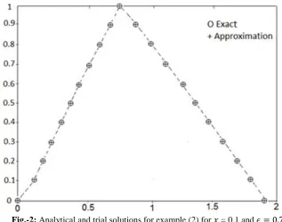
Fig.-2: Analytical and trial solutions for example (2) for 𝑥𝑥 = 0.1 and 𝜖𝜖= 0.7

Example 3: Consider the homogeneous second order FDE: _𝑦𝑦ˊˊ₍_𝑥𝑥₎₋₄_𝑦𝑦₍ˊ_𝑥𝑥_{) + 4}_𝑦𝑦₍_𝑥𝑥₎ =0, _{𝑥𝑥 ∈}_[0,1].

[𝑦𝑦(0)]𝑟𝑟 = [2 +𝑟𝑟 ,4− 𝑟𝑟], [ 𝑦𝑦ˊ(0)]𝑟𝑟 =[5 + r , 7 - r], r ϵ [0,1].

E(𝑥𝑥,0.2)

𝑦𝑦𝑡𝑡(𝑥𝑥,0.2)

𝑦𝑦𝑎𝑎(𝑥𝑥,0.2)

E(𝑥𝑥,0.2)

𝑦𝑦𝑡𝑡(𝑥𝑥,0.2)

𝑦𝑦𝑎𝑎(𝑥𝑥,0.2)

_𝑥𝑥

0.0000000 0.0000212 0.0000076 0.0000372 0.0000089 0.0000079 0.0000121 0.0000036 0.0000016 0.0000223 0.0000030 0.6788854

0.7199199 0.7662744 0.8190363 0.8794966 0.9496574 1.0320011 1.1299366 1.2484338 1.3946728 1.5797694 0.6788854

0.7199411 0.7662820 0.8189991 0.8795055 0.9496653 1.0319890 1.1299402 1.2484354 1.3946951 1.5797724 0.0000000

0.0000659 0.0000079 0.0000479 0.0000199 0.0000059 0.0000624 0.0000088 0.0000846 0.0000158 0.0000021 0.2236068

0.2254873 0.2272736 0.2291883 0.2310662 0.2329901 0.2350173 0.2369680 0.2389134 0.2410563 0.2431805 0.2236068

0.2254214 0.2272657 0.2291404 0.2310463 0.2329842 0.2349549 0.2369592 0.2389980 0.2410721 0.2431826 0.10

(9)

𝑦𝑦𝑎𝑎(𝑥𝑥,𝑟𝑟) = [(2 +𝑟𝑟) 𝑒𝑒2𝑥𝑥 +(1− 𝑟𝑟)𝑥𝑥𝑒𝑒2𝑥𝑥, (4− 𝑟𝑟)𝑒𝑒2𝑥𝑥 +(𝑟𝑟 −1)𝑥𝑥𝑒𝑒2𝑥𝑥 ].

𝑦𝑦𝑡𝑡(𝑥𝑥,𝑟𝑟) = [2 +𝑟𝑟, 4− 𝑟𝑟] + [5 +𝑟𝑟, 7− 𝑟𝑟]𝑥𝑥+𝑥𝑥2[𝑁𝑁(𝑥𝑥,𝑝𝑝)]𝑟𝑟 .

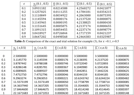
Table (3) shows the exact solution and the trial solution for 𝑥𝑥 =0.1 and r= 0.5. Numerical results for 𝜖𝜖= 0.4 and r= 0.5 can be found in table (4)

Note that for 𝑥𝑥 =0.1 and r=0.5, the fuzzy exact solution is:

𝑦𝑦𝑎𝑎 (0.1, 0.5) = [3.11457703, 4.21383952], 𝐻𝐻(𝑥𝑥) = 1.11𝜖𝜖𝑎𝑎𝑛𝑛𝑑𝑑 for 𝜖𝜖=0.4 and r=0.5, the fuzzy exact solution is:

𝑦𝑦𝑎𝑎 (𝑥𝑥, 0.5) = [2.5 𝑒𝑒2𝑥𝑥+ 0.5 𝑥𝑥𝑒𝑒2𝑥𝑥, 3.5 𝑒𝑒2𝑥𝑥 - 0.5 x 𝑒𝑒2𝑥𝑥],𝐻𝐻(𝑥𝑥)=0.4 (𝑥𝑥2+𝑥𝑥+1).

Table-3: Comparison of the exact and trial solution for example (3), for 𝑥𝑥 =0.1, r=0.5

Table-4: Comparison of the exact and trial solution for example (3), for 𝜖𝜖=0.4, r=0.5

Example (4): Consider the nonhomogeneous second order FDE: 𝑦𝑦ˊˊ+ 4𝑦𝑦= 2𝑐𝑐𝑜𝑜𝐸𝐸𝑥𝑥, 𝑥𝑥 ∈[0,1].

[𝑦𝑦(0)]𝑟𝑟 = [2𝑟𝑟 , 4−2𝑟𝑟], [𝑦𝑦ˊ(0)]𝑟𝑟 = [−2 + 2𝑟𝑟 , 2−2𝑟𝑟], 𝑟𝑟𝜖𝜖 [0,1].

𝑦𝑦𝑎𝑎(𝑥𝑥,𝑟𝑟) = [( 2𝑟𝑟 −2₃)𝑐𝑐𝑜𝑜𝐸𝐸2𝑥𝑥+ (𝑟𝑟 −1)𝐸𝐸𝑖𝑖𝑛𝑛2𝑥𝑥+ 2₃ cos𝑥𝑥,( 10₃ −2𝑟𝑟) 𝑐𝑐𝑜𝑜𝐸𝐸2𝑥𝑥+ (1− 𝑟𝑟)𝐸𝐸𝑖𝑖𝑛𝑛2𝑥𝑥+ 2₃ cos𝑥𝑥].

𝑦𝑦𝑡𝑡(𝑥𝑥 , r) = [2r, 4-2r] + [-2 + 2r, 2-2r]𝑥𝑥 + 𝑥𝑥2 [𝑁𝑁(𝑥𝑥 ,𝑝𝑝)]𝑟𝑟.

Table (5) shows the exact and the trial solution for 𝑥𝑥 = 1 and r = 0.7.

Numerical results for 𝜖𝜖 = 0.8 and r = 0.7 can be found in table (6).

Note that for 𝑥𝑥 = 1 and r= 0.7, the fuzzy exact solution is:

𝑦𝑦𝑎𝑎 (1, o.7) = [-0.21776204, -0.17155979], 𝐻𝐻(𝑥𝑥) = 3𝜖𝜖

And for 𝜖𝜖 = 0.8, r = 0.7, the fuzzy exact solution is

𝑦𝑦𝑎𝑎 (𝑥𝑥 , 0.7) = [o.73333 cos2𝑥𝑥 – 0.3 sin2𝑥𝑥 + 2₃ cos𝑥𝑥 , 1.93333 cos2𝑥𝑥 + 0.3 sin2𝑥𝑥 + 23 cos𝑥𝑥].

E(0.1 , 0.5)

𝑦𝑦𝑡𝑡(0.1 , 0.5)

E(0.1 , 0.5)

𝑦𝑦𝑡𝑡(0.1 , 0.5)

𝜖𝜖 0.0421877 0.0354215 0.0075395 0.0000875 0.0000430 0.0000655 0.0098779 0.0421237 0.0325987 4.2560272 4.1784181 4.2063000 4.2137520 4.2138825 4.2137174 4.2237174 4.1717159 4.2464383 0.0214588 0.0111255 0.0034922 0.0000176 0.0000195 0.0005875 0.0054455 0.0726844 0.0498568 3.0931182 3.1257025 3.1110849 3.1145594 3.1145965 3.1151645 3.1091315 3.0418927 3.0647202 0.1 0.2 0.3 0.4 0.5 0.6 0.7 0.8 0.9

_𝑥𝑥 _𝑦𝑦_𝑎𝑎 (_𝑥𝑥,0.5) _𝑦𝑦_𝑡𝑡 (_𝑥𝑥,o.5) _E (_𝑥𝑥,0.5) _𝑦𝑦_𝑎𝑎 (_𝑥𝑥,0.5) _𝑦𝑦_𝑡𝑡 (_𝑥𝑥,o.5) _E(_𝑥𝑥,o.5)

(10)

Table-5: Comparison of the exact and the trial solution for example (4) for 𝑥𝑥 = 1 and r = 0.7.

𝑥𝑥 𝑦𝑦_𝑎𝑎 (𝑥𝑥,0.7) 𝑦𝑦_𝑡𝑡 (𝑥𝑥,o.7) E (𝑥𝑥,0.7) 𝑦𝑦_𝑎𝑎(𝑥𝑥,o.7) 𝑦𝑦_𝑡𝑡(𝑥𝑥,o.7) E(𝑥𝑥,o.7) 0 0.1 0.2 0.3 0.4 0.5 0.6 0.7 0.8 0.9 1 1.4000000 1.3224508 1.2119969 1.0727444 0.9097521 0.7288354 0.5363410 0.3389024 0.1431861 -0.044363 -0.217762 1.4000000 1.3223751 1.2120015 1.0727385 0.9097470 0.7289057 0.5363339 0.3389635 0.1431835 -0.044339 -0.217759 0.0000000 0.0000757 0.0000046 0.0000059 0.0000051 0.0000703 0.0000072 0.0000611 0.0000026 0.0000240 0.0000030 2.6000000 2.6177966 2.5509211 1.9773386 2.1762138 1.8820808 1.5303938 1.1341329 0.7078908 0.2673036 -0.171559 2.6000000 2.6177966 2.5509281 1.9773348 2.1761849 1.8821797 1.5303961 1.1340851 0.7078820 0.2673062 -0.171563 0.0000000 0.0000643 0.0000070 0.0000038 0.0000289 0.0000989 0.0000023 0.0000478 0.0000088 0.0000026 0.0000040

Table-6: Comparison of the exact and the trial solution for example (4), for 𝜖𝜖 = 0.8 and r = 0.7.

8. CONCLUSIONS

In this paper, we presented a hybrid approach based on modified fuzzy neural networks for solving fuzzy differential equations. We demonstrate, for the first time, the ability of modified fuzzy neural networks to approximate the solutions of FDEs. By comparing our results with the results obtained by using numerical methods, it can be observed that the proposed method yields more accurate approximations. Even better results may be possible if one uses more neurons or more training points. Moreover, after solving a FDE the solution is obtainable at any arbitrary point in the training interval (even between training points). The main reason for using modified fuzzy neural networks was their applicability in function approximation. Further research is in progress to apply and extend this method to solve fuzzy partial differential equations FPDEs.

REFERENCES

1. S. Abbasbandy and T. Allahviranloo, Numerical solution of fuzzy Differential equations by Runge-Kutta method, J. Sci. Teacher Training University, 1(3), 2002.

2. S. Abbasbandy and T.Allahviranloo, Numerical solution of fuzzy Differential equations by Taylor method, Journal of Computational Methods in Applied Mathematics, 2 (2002), 113-124.

3. T. Allahviranloo, N. Ahmady, and E. Ahmady, Numerical solution of fuzzy Differential equations by predictor- corrector method, Information Sciences, 177 (2007), 1633-1647.

4. T.Allahviranloo, E. Ahmady, and N. Ahmady, Nth- order fuzzy linear Differential equations , Information Sciences, 178 (2008), 1309-1324.

5. T. Allahviranloo,N. A. Kiani, and N. Motamedi, Solving fuzzy differential equations by differential transformation method, Information Sciences,179 (2009), 956-966. 6. S.Abbasbandy, M. Otadi, Numerical solution of fuzzy polynomials by fuzzy neural network, Appl. Math.

Comput. 181(2006)1084 -1089.

7. S.Abbasbandy, M. Otadi, M. Mosleh, Numerical solution of a system of fuzzy polynomials by fuzzy neural network, Information sciences 178 (2008) 1948 – 1960.

8. B. Bede and S. G. Gal, Generalizations of the differentiability of fuzzy number- valued functions with applications to fuzzy differential equations, Fuzzy Sets and Systems, 151 (2005), 581 – 599.

9. J.J. Buckley and T. Feuring, Fuzzy differential equations, Fuzzy Sets and Systems, 110 (2000), 43 – 54. 10. P.Diamond, Stability and periodicity in fuzzy differential equations, IEEE Trans, Fuzzy Systems, 8 (2000),

583 – 590.

E (1 , 0.7)

𝑦𝑦𝑡𝑡(1, 0.7)

E (1 , 0.7)

𝑦𝑦𝑡𝑡(1 , 0.7)

(11)

11. P. Diamond, Brief note on the variation of constants formula for fuzzy differential equations, Fuzzy Sets and Systems, 129 (2002), 65 – 71.

12. S. Ezadi, N. Parandin, A. Ghomashi, Numerical solution of fuzzy differential equations based on semi-Taylor by using neural network, Journal of basic and applied scientific research (2013), 477-482.

13. B. Ghazanfari and A. Shakerami, Numerical solution of fuzzy differential equations extended Runge – Kutta- like formulae of order 4, Fuzzy Sets and Systems, 189 (2011), 74 – 91.

14. D.N.Georgiou, J.J.Nieto, and R. Rodriguez-Lopez, Initial value problems for higher-order fuzzy differential equations, Nonlinear Anal.,63 (2005),587-600.

15. K. Hornick, M. Stinchcombe, Multi-layer feed forward networks are universal approximators, Neural Networks 2(1989)359 - 366.

16. O. Kaleva, Fuzzy differential equations, Fuzzy Sets and Sydtems, 24 (1987), 301 – 317. 17. T.Khanna, Foundations of neural networks, Addison-Wesly, Reading, MA,(1990).

18. A. Kastan and K. Ivaz, Numerical solution of fuzzy differential equations by Nystrom method. Chaos, Solitons and Fractals, 41(2009), 859 – 868.

19. H. Lee and I. S. Kang, Neural algorithms for solving differential equations, Journal of Computational Physics, 91 (1990), 110-131.

20. M.Mosleh, Fuzzy neural network for solving a system of fuzzy differential equations, Applied Soft Computing, 13(2013), 3597-3607.

21. M.Mosleh, T. Allahviranloo, and M.Otadi, Evaluation of fully fuzzy regression models by fuzzy neural network, Neural Comput and Applications,21 (2012), 105 – 112.

22. A. J. Meade and A.A. Fernandez, The numerical solution of linear ordinary differential equations by feed-forward neural network, Mathematical and Computer Modelling, 19(12) (1994), 1 – 25.

23. M. Mosleh, M. Otadi, Simulation and evaluation of fuzzy differential equation by fuzzy neural network, Applied soft computing 12(2012)2817 - 2827.

24. M.Mosleh,M.Otadi, Solving the second order fuzzy differential equations by fuzzy neural network, Journal of Mathematical Extension 81 (2014), 11 – 27.

25. M.Mosleh,M.Otadi, and S.Abbasbandy, Evaluation of fuzzy regression models by fuzzy neural network, Journal of Computational and Applied Mathematics,234 (2010), 825 – 834.

26. M.Mosleh,M.Otadi, and S.Abbasbandy, Fuzzy polynomial regression with fuzzy neural network, Applied Mathematical Modeling,35 (2011), 5400 – 5412.

27. A.Malek and R. Shekari Beidokhti, Numerical solution for high order differential equations using a hybrid neural network-Optimization method, Appl. Math. Comput. 183 (2006), 260 – 271.

28. J .J. Nieto, The Cauchy problem for continuous fuzzy differential equations, Fuzzy Sets and Systems, 102 (1999), 259 – 262.

29. J.J. Nieto and R.Rodriguez-Lopez, Bounded solutions for fuzzy differential and integral equations, Chaos, Solitons and Fractals, 27 (2006), 1376 – 1386.

30. M. Otadi, M. Mosleh, S. Abbasbandy, solving fuzzy linear system by neural network and applications in Economics, Journal of mathematics extension (2011)47 - 66.

31. M. Otadi. M.Mosleh, and S. Abbasbandy, Numerical solution of fully fuzzy linear systems by fuzzy neural network, Soft Computing, 15 (2011), 1513 – 1522.

32. H. Ouyang and Y. Wu, On fuzzy differential equations, Fuzzy Sets and Systems, 32 (1989), 321 – 325.

Source of support: Nil, Conflict of interest: None Declared

[Copy right © 2015. This is an Open Access article distributed under the terms of the International Journal of Mathematical Archive (IJMA), which permits unrestricted use, distribution, and reproduction in any

medium, provided the original work is properly cited.]