A NUMERICAL TECHNIQUE FOR THE SOLUTION OF GENERAL EIGHTH ORDER BOUNDARY VALUE PROBLEMS: A FINITE DIFFERENCE METHOD

(1)

A NUMERICAL TECHNIQUE FOR THE SOLUTION OF

GENERAL EIGHTH ORDER BOUNDARY VALUE

PROBLEMS: A FINITE DIFFERENCE METHOD

Pramod Kumar Pandey

Dyal Singh College (University of Delhi), New Delhi, India

Abstract:In this article, we present a novel finite difference method for the numerical solution of the eighth order boundary value problems in ordinary differential equations. We have discretized the problem by using the boundary conditions in a natural way to obtain a system of equations. Then we have solved system of equations to obtain a numerical solution of the problem. Also we obtained numerical values of derivatives of solution as a byproduct of the method. The numerical experiments show that proposed method is efficient and fourth order accurate.

Key words: Boundary value problem, Eighth order equation, Finite difference method, Fourth order method.

1. Introduction

In the present article we have considered general eighth order boundary value problem of the following form:

u(8)(x) =f(x, u, u′, u′′, u(3), u(4), u(5), u(6), u(7)), a < x < b (1.1)

and the boundary conditions are

u(a) =α1, u′′(a) =α2, u(4)(a) =α3, u(6)(a) =α4, u(b) =β1, u′′(b) =β2, u(4)(b) =β3 and u(6)(b) =β4,

whereu(x) and forcing functionf(x, u, u′, u′′, u(3), u(4), u(5), u(6), u(7)) are real and smooth function in [a,b] andα1, α2, α3, α4, β1, β2, β3 and β4 are constant.

The above eight order boundary value problem arises in physics such as fluid dynamics, vibra-tions and so on [1, 2]. For the detail discussion on the existence and uniqueness of the solution of higher order differential equations and corresponding BVPs, reader can refer [3]. So we have assumed that there exists a unique solution to boundary value problem (1.1).

In general it is difficult to obtain analytical solution of the (1.1) for the arbitrary forcing function f. Hence we desire some numerical technique for its numerical solution. We have some numerical methods for either same or different source function as in problem (1.1), for examples Galerkin Method [4,5], variational iterational technique [6], finite difference method [7], Adomian decomposition method [8] and references there in.

(2)

well structured system of equations for the numerical solution of problem (1.1) and some other by-products.

We have presented our work in this article as follows. In Section 2 we have proposed our finite difference method and in Section 3 the derivation of the proposed finite difference method. In Section 4 we have tested proposed method on model problems and short discussion on numerical results. A summary on development and performance of the proposed method are presented in Section 5.

2. The Difference Method

Let us assume problem (1.1) posses solution and it will be u(x) such that

u(8)(x) =f(x, u, u′, u′′, u(3), u(4), u(5), u(6), u(7)), a < x < b (2.1) and the boundary conditions are

u(a) =α1, u′′(a) =α2, u(4)(a) =α3, u(6)(a) =α4, u(b) =β₁, u′′(b) =β₂, u(4)(b) =β₃ and u(6)(b) =β₄,

where source function f is regular and differentiable in [a, b]. To derive and develop a numerical method for the solution of the problem we need following definitions and approximations.

To introduce finite number of discrete mesh points we partition the interval [a, b] in which the solution of problem (1.1) is desired. In these subintervals discrete mesh points a ≤ x0 < x1 < x2 < · · · < xN+1 ≤ b are generated by using uniform step length h such that xi = a+ih, i= 0,1,2, . . . , N + 1. We wish to determine the numerical solution of the problem (1.1) at these discrete mesh points xi. We denote the numerical approximation of u(x) and f respectively byui

and fi. Hence, the boundary value problem (1.1) may be written as

u(8)i =Fi, (2.2)

whereFi =f(xi, ui, u′_{i, u}′′

i, u (3) i , u

(4) i , u

(5) i , u

(6) i , u

(7)

i ) at the discrete mesh pointx=xi,i= 1,2, . . . , N.

Let

u′

i =

1

2h(ui+1−ui−1)− h

12(u ′′

i₊₁−u′′i−1), (2.3)

u(3)i =

1 2h(u

′′

i₊₁−u′′i₋₁)− h

12(u

(4) i₊₁−u

(4)

i−1), (2.4)

u(5)i =

1 2h(u

(4) i₊₁−u

(4) i−1)−

h

12(u

(6) i₊₁−u

(6)

i−1), (2.5)

u(7)i =

1 2h(u

(6) i₊₁−u

(6)

i₋₁), (2.6)

u′

i₊₁ =

1

2h(ui+1−ui−1) + h

3(u ′′

i₊₁+ 2u′′i), (2.7)

u′

i−1 =

1

2h(ui+1−ui−1)− h

3(2u ′′

i +u

′′

i−1), (2.8)

u(3)i₊₁=

1 2h(u

′′

i₊₁−u′′i−1) + h

3(u

(4) i₊₁+ 2u

(4)

i ), (2.9)

u(3)i₋₁=

1 2h(u

′′

i₊₁−u

′′

i−1)− h

3(2u

(4) i +u

(4)

i₋₁), (2.10)

u(5)i₊₁=

1 2h(u

(4) i₊₁−u

(4) i−1) +

h

3(u

(6) i₊₁+ 2u

(6)

i ), (2.11)

u(5)i−1=

1 2h(u

(4) i₊₁−u

(4) i−1)−

h

3(2u

(6) i +u

(6)

(3)

u(7)i₊₁ =

1 2h(3u

(6) i₊₁−4u

(6) i +u

(6)

i₋₁), (2.13)

u(7)i₊₁=

1 2h(−u

(6) i₊₁+ 4u

(6) i −3u

(6)

i₋₁), (2.14)

Fi₊₁ =f(xi₊₁, ui₊₁, u′_i₊₁, u′′i₊₁, u (3) i₊₁, u

(4) i₊₁, u

(5) i₊₁, u

(6) i₊₁, u

(7)

i₊₁), (2.15) Fi₋₁ =f(xi₋₁, ui₋₁, u′_i₋₁, u′′i−1, u

(3) i−1, u

(4) i−1, u

(5) i−1, u

(6) i−1, u

(7)

i−1), (2.16) u(7)i =u

(7) i −

8971

202084h(Fi+1−Fi−1), (2.17) d

u(7)i =u (7) i −

739

16620h(Fi+1−Fi−1), (2.18) d

d

u(7)i =u (7) i −

155

732h(Fi+1−Fi−1), (2.19) g

g

u(7)i =u (7) i −

1

20h(Fi+1−Fi−1), (2.20)

Fi =f(xi, ui, u′_{i, u}′′

i, u (3) i , u

(4) i , u

(5) i , u

(6) i , u

(7)

i ), (2.21)

b

Fi =f(xi, ui, u′i, u′′i, u (3) i , u

(4) i , u

(5) i , u

(6) i ,

d

u(7)i ), (2.22)

bb

Fi =f(xi, ui, u′

i, u

′′

i, u (3) i , u

(4) i , u

(5) i , u

(6) i ,

d d

u(7)i ), (2.23)

ee

Fi =f(xi, ui, u′

i, u

′′

i, u (3) i , u

(4) i , u

(5) i , u

(6) i ,

g g

u(7)i ) (2.24)

at these node x =xi, i= 1, .., N. Following the ideas in [9], thus we propose our finite difference method for a numerical solution of problem (2.2),

−720(ui+1−2ui+ui−1) + 360h2(u′′i₊₁+u′′i₋₁)−150h4(u (4) i₊₁+u

(4)

i−1) + 61h6(u (6) i₊₁+u

(6) i−1)

= h

8

1260(5902Fi+1+ 50521Fi+ 5902Fi−1), 24(u′′i₊₁−2u

′′

i +u

′′

i−1)−12h2(u (4) i₊₁+u

(4)

i−1) + 5h4(u (6) i₊₁+u

(6) i−1)

= h

6

840(323Fi+1+ 2770Fbi+ 323Fi−1),

−2(u(4)i₊₁−2u (4) i +u

(4)

i−1) +h2(u (6) i₊₁+u

(6) i−1) =

h4

90(7Fi+1+ 61Fbbi+ 7Fi−1),

u(6)i₊₁−2u (6) i +u

(6) i−1 =

h2

12(Fi+1+ 10Feei+Fi−1).

(2.25)

If the forcing functionf in problem (1.1) is linear then the system of equations (2.25) will be linear otherwise we will obtain system of nonlinear equations.

3. Derivation of the Difference Method

In this section we shall out line the derivation of the proposed method (2.25). Using Taylor series and undetermine coefficients method, it is to verify that the following discretization

−720(ui+1−2ui+ui−1) + 360h2(u′′i₊₁+u′′i₋₁)−150h4(u (4) i₊₁+u

(4)

i−1) + 61h6(u (6) i₊₁+u

(6) i−1)

= h

8

1260(5902Fi+1+ 50521Fi + 5902Fi−1),

(4)

for the solution of problem (1.1) when source function F =f(x, u) is ofO(h4). To discretize prob-lem (1.1) at discrete points, we need approximations of order four for the source functionF. So let outline method to obtain fourth order approximation for the forcing functionsF.

Though the approximations (2.3)–(2.5) and (2.7)–(2.12) are fourth order approximation tou′i,..

respectively. But some approximations defined in section 2 are not of order four. From (2.6), let expand each term in right in Taylor series about a pointx=xi and simplify, we have

u(7)i =u (7) i +

h2

6 u

(9) i +O(h

4₎ _(3.2)

From (2.13) and (2.14) respectively, we have

u(7)i₊₁ =u (7) i₊₁−

h2

3 u

(9) i −

h3

12u

(10) i +O(h

4₎ _(3.3)

u(7)i−1 =u (7) i−1−

h2

3 u

(9) i +

h3

12u

(10) i +O(h

4₎ _(3.4)

Let us define

u(7)i =u (7)

i +a1h(Fi₊₁−Fi−1) (3.5)

wherea1 is free parametric constant and to be determined under appropriate condition.

Using (3.3) in (2.15), we will obtain

Fi₊₁=Fi₊₁+ (− h2

3 u

(9) i −

h3

12u

(10) i )(

∂f

∂u(7))i+1+O(h

4₎ _(3.6)

and similarly from (2.16) and (3.4) we have

Fi−1=Fi−1+ (− h2

3 u

(9) i +

h3

12u

(10) i )(

∂f

∂u(7))i−1+O(h

4₎ _(3.7)

Thus, using (3.2), (3.6) and (3.7) in (3.5), we have

u(7)_i ₌_u(7) i + (

h2

6 + 2a1h

2₎_u(9)

i +O(h4) (3.8)

Using (3.8) in (2.21) and simplify, we have

Fi =Fi+ (h

2

6 + 2a1h

2₎_u(9) i (

∂f

∂u(7))i+O(h

4₎ _(3.9)

Let us consider the expression, 5902Fi₊₁+ 50521Fi+ 5902Fi−1 and simplify this expression using

(3.6), (3.7) and (3.9). We will obtain

5902Fi₊₁+ 50521Fi+ 5902Fi−1 = 5902Fi+1+ 50521Fi+ 5902Fi−1

+h

2

6 (26913 + 606252a1)(u

(9) ∂f

∂u(7))i+O(h

4₎ (3.10)

Thus from (3.10), we conclude that 5902Fi₊₁ + 50521Fi + 5902Fi−1 will provide fourth order

approximation to 5902Fi₊₁+ 50521Fi+ 5902Fi−1 if

a1 =

(5)

i.e.

5902Fi₊₁+ 50521Fi+ 5902Fi−1 = 5902Fi+1+ 50521Fi+ 5902Fi−1+O(h4) (3.11)

Similarly, we can find other fourth order approximations of the terms in (2.25)

323Fi₊₁+ 2770Fbi+ 323Fi−1= 323Fi+1+ 2770Fi+ 323Fi−1+O(h4)

7Fi₊₁+ 61Fbbi+ 7Fi−1= 7Fi+1+ 61Fi+ 7Fi−1+O(h4)

Fi₊₁+ 10Feei+Fi−1=Fi+1+ 10Fi+Fi−1+O(h4)

(3.12)

Thus by using (3.11) and (3.12) in (3.1), we will get our proposed fourth order difference method (2.25) for the numerical solution of the problem (1.1). Moreover we are getting the numerical value of the derivative of the solution of the problem (1.1) as a byproduct of the method.

4. Numerical Results

To test the computational efficiency of method (2.25), we have considered three model problems. In each model problem, we took uniform step size h. In Table 1, Table 3 and Table 4, we have shown M AEU, M AEV, M AEW and M AES the maximum absolute error in the solution u(x), second, fourth and sixth derivatives of solutionu(x) of the problems (1.1) respectively for different values ofN. We have used the following formulas in computation ofM AEU,M AEV,M AEW and

M AES:

M AEU = max

1≤i≤N|Ui−u(xi)|

M AEV = max

1≤i_≤N

Ui′′−u

′′₍_xi₎

M AEW = max

1≤i≤N

Ui(4)−u (4)₍_xi₎

M AES = max

1≤i≤N

Ui(6)−u(6)(xi)

where u(xi) and Ui are respectively exact and computed value of the solution of the problem and similarly we have defined others terms in the above expression. The order of the convergence of the proposed method (2.25) is estimated by using following formula,

ON = logr(

M AEUN M AEUrN)

wherer is ratio of the uniform step lengths h.

We have used Newton Raphson and Gauss Seidel method to solve system of nonlinear/linear equations (2.25). All computations were performed on a Windows 2007 Ultimate operating system in the GNU FORTRAN environment version 99 compiler (2.95 of gcc) on Intel Core i3-2330M, 2.20 GHz PC. The solutions are computed on N nodes and iteration is continued until either the maximum difference between two successive iterates is less than 10−9 _{or the number of iteration}

reached 103.

Problem 1. The model linear problem in [4] given as:

u(8)(x) =−u(7)−2u(6)−2u(5)−2u(4)−2u(3)−2u′′−u′−u+ 14 cos(x)−4(4 +x) sin(x),

(6)

subject to boundary conditions

u(1) = 0, u′′(1) = 4 cos(1) + 2 sin(1), u(4)(1) =−8 cos(1)−12 sin(1),

u(6)(1) = 12 cos(1) + 30 sin(1), u(0) = 0, u′′(0) = 0, u(4)(0) = 0 and u(6)(0) = 0.

The analytical solution of the problem is u(x) = (x2 −1) sin(x). The M AEU, M AEV, M AEW

and M AES were computed by method (2.25) for different values of N and presented in Table 1.

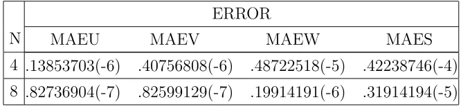
Problem 2. The model linear problem in [5] given as:

u(8)(x) =−sin(x)u(5)−(1−x2)u(4)−u(x) + (3 + sin(x)−x2) exp(x), 0< x <1,

u(0) = 1, u′′(0) = 1, u(4)(0) = 1, u(6)(0) = 1, u(1) = exp(1), u′′(1) = exp(1), u(4)(1) = exp(1) and u(6)(1) = exp(1).

The analytical solution of the problem is u(x) = exp(x). The M AEU, M AEV, M AEW and

M AES were computed by method (2.25) for different values of N and presented in Table 2.

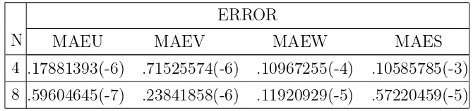
Problem 3. Consider the following non-linear model problem given as:

u(8)(x) =−sin(u(x))u(3)+f(x), 0< x <1,

u(0) = 0, u′′(0) =−2, u(4)(0) = 0, u(6)(0) = 8, u(1) = (1−exp(1)) sin(1), u′′(1) =−2 exp(1) cos(1)−sin(1), u(4)(1) = (4 exp(1) + 1) sin(1),

and u(6)(1) = 8 exp(1) cos(1)−sin(1).

wheref(x) is calculated so that the analytical solution of the problem isu(x) = (1−exp(x)) sin(x). The M AEU,M AEV,M AEW and M AES were computed by method (2.25) for different values of N and presented in Table 3.

Table 1. Maximum absolute error (Problem 1).

ERROR

N MAEU MAEV MAEW MAES

4 .13351440(-4) .13279915(-3) .15587807(-2) .47683716(-3) 8 .11324883(-5) .12874603(-4) .15258789(-3) .34332275(-4) 16 .29802322(-7) .23841858(-6) .66757202(-5) .11444092(-4)

ERROR

(7)

ERROR

4 .17881393(-6) .71525574(-6) .10967255(-4) .10585785(-3) 8 .59604645(-7) .23841858(-6) .11920929(-5) .57220459(-5)

The numerical results obtained in numerical experiment in considered model problems validate the fourth order accuracy. Also we have fourth order accurate numerical value of the second, fourth and sixth derivative of solution of problem as a byproduct of the proposed method (2.25).

5. Conclusion

In the present article, we have described a novel finite difference method for the numerical solution of the eighth order BVP’s in ordinary differential equations. We have transformed the problem into system of algebraic equations at mesh pointsx=xi, i= 1,2, . . . , N. Then the system of algebraic equations is solved for the solution of the problem. The proposed method in numerical experiments has shown its efficiency and fourth order accuracy. The advantage of the proposed method is that we also get fourth order accurate numerical value of the derivatives of the solution as byproduct.

6. Acknowledgements

The author is grateful to the anonymous reviewers and editor for their valuable suggestions, which substantially improved the standard of the paper.

REFERENCES

1. Chandrasekhar S.Hydrodynamics and Hydromagnetic Stability. The Clarendon Press, Oxford, 1961. 2. Shen Y.I. Hybrid damping through intelligent constrained layer layer treatments. ASME Journal of

Vibration and Acoustics, 1994. Vol. 116, no. 3. P. 341–349.DOI: 10.1115/1.2930434

3. Agarwal R.P. Boundary Value Problems for Higher Order Differential Equations. Singapore: World Scientific, 1986.DOI: 10.1142/0266

4. Viswanadham K.N.S.K., Ballem S. Numerical solution of eighth order boundary value problems by Galerkin method with quintic B-splines.International Journal of Computer Applications, 2014. Vol. 89, no. 15. P. 7–13.DOI: 10.5120/15705-4562

5. Reddy S.M. Numerical solution of eighth order boundary value problems by Petrov-Galerkin method with quintic B-splines as basic functions and septic B-splines as weight functions. In-ternational Journal of Engineering and Computer Science, 2016, Vol. 5, no. 09. P. 17894–17901. http://ijecs.in/index.php/ijecs/article/view/2439/2254

6. Siddiqi S.S., Akram G. and Zaheer S. Solution of eighth order boundary value problems using Variational iteration technique.European Journal of Scientific Research, 2009. Vol. 30. P. 361–379.

7. Boutayeb A., Twizell E.H. Finite-difference methods for the solution of special eighth-order boundary-value problems. International Journal of Computer Mathematics, 1993. Vol. 48, no. 1–2. P. 63–75. DOI: 10.1080/00207169308804193

8. Inc M., Evans D.J. An efficient approach to approximate solutions of eighth-order boundary-value problems. International Journal of Computer Mathematics, 2004. Vol. 81, no. 6. P. 685–692. DOI: 10.1080/0020716031000120809