Volume 39 (2011)
Graph Computation Models
Selected Revised Papers from the
Third International Workshop on
Graph Computation Models (GCM 2010)
Formal Specification of Model Transformations by Triple Graph
Grammars with Application Conditions
Ulrike Golas, Hartmut Ehrig and Frank Hermann
26 pages
Guest Editors: Rachid Echahed, Annegret Habel, Mohamed Mosbah Managing Editors: Tiziana Margaria, Julia Padberg, Gabriele Taentzer
Formal Specification of Model Transformations by Triple Graph
Grammars with Application Conditions
Ulrike Golas1, Hartmut Ehrig2and Frank Hermann23
1[email protected], Konrad-Zuse-Zentrum f¨ur Informationstechnik Berlin, Germany 2ehrig|[email protected], Technische Universit¨at Berlin, Germany 3[email protected], SnT, Universit´e du Luxembourg, Luxembourg
Abstract: Triple graph grammars are a successful approach to describe exogenous model transformations, i.e. transformations between models conforming to differ-ent meta-models. Source and target models are related by some connection part, triple rules describe the simultaneous construction of these parts, and forward and backward rules can be derived modeling the forward and backward model transfor-mations. As shown already for the specification of visual models by typed attributed graph transformation, the expressiveness of the approach can be enhanced signifi-cantly by using application conditions, which are known to be equivalent to first order logic on graphs.
In this paper, we extend triple rules with a specific form of application conditions, which enhance the expressiveness of formal specifications for model transforma-tions. We show how to extend results concerning information preservation, termi-nation, correctness, and completeness of model transformations to the case with application conditions. We illustrate our approach and results with a model trans-formation from statecharts to Petri nets.
Keywords:model transformation, triple graph grammar, application condition
1
Introduction
completeness of model transformations have been studied already in [EEH08, EEHP09] based on triple rules without NACs, where the decomposition and composition theorem for triple graph transformation sequences in [EEE+07] plays a fundamental role. In [EHS09], this theorem has been extended to triple rules with NACs, but not yet to nested application conditions [HP09].
It is the main aim of this paper to extend the theory of model transformations based on TGGs to rules with nested application conditions, short application conditions, in order to enhance the expressiveness of model transformations including the generation of the source and target languages by corresponding source and target rules. We show that the decomposition and com-position theorem can be extended to rules with application conditions. This allows to enhance the expressiveness of model transformations and to extend termination, correctness, completeness, and backward information preservation to this more general framework.
As a case study, we consider a model transformation from statecharts to Petri nets, where we use a combination of positive and negative application conditions and boolean operators as avail-able in the framework of general application conditions, but not in the more restrictive framework of NACs. In our example, only one level of nesting is sufficient to model the necessary condi-tions, but the theory is developed for more complex situations as introduced in [Gol11].
This paper is organized as follows. InSection 2, we review triple rules and application con-ditions. We illustrate our approach with a model transformation from statecharts to Petri nets in Section 3. This case study is used as illustrating example inSection 4, where we define model transformations based on TGGs with application conditions leading to termination, correctness, completeness, and backward information preservation. A conclusion including related and future work is presented inSection 5.
We assume the reader to be familiar with the basics of UML statecharts [OMG09], Petri nets [Pet80], and graph transformation in the double pushout approach [EEPT06].
2
Review of Triple Graph Grammars and Application Conditions
Triple graph grammars [Sch94] are a well known approach for bidirectional model transforma-tions. In [KS06], the basic concepts of triple graph grammars are formalized in a set-theoretical way, which is generalized and extended in [EEE+07] to typed, attributed graphs.
A triple graph G= (GS sG
←GC tG
→GT) consists of graphsGS, GC, and GT, called source, connection, and target component, and two graph morphismssGandtGmapping the connection to the source and target components. A triple graph morphism f :G1→G2 matches the single
components and preserves the connection part.
The typing of a triple graph is done in the same way as for standard graphs via a type graph
T G - in this case a triple type graph - and a typing morphism typeG from the graph G into this type graph leading to the typed triple graph(G,typeG). A typed triple graph morphism
f :(G1,typeG1)→(G2,typeG2)is a triple graph morphism f such thattypeG2◦f=typeG1.
adhesive HLR categories [EEPT06] which allows us to instantiate the theory to transformations of triple graphs. The categorical foundations of weak adhesive HLR categories are not essential to understand this paper.
L R
G H
LS LC LT
GS GC GT
RS RC RT
HS HC HT
tr
f
m n
sL tL
sG tG
mS mC sR mT tR
sH tH
nS nC nT
trS trC trT
fS fC fT
(1)
A triple rule tr = (L →tr R)
consists of triple graphs L and
R, and anM-morphismtr:L→
R. Since triple rules are non-deleting, we do not need a span of morphisms for a rule. Adirect triple transformation G===tr,m⇒H
of a triple graphGvia a triple ruletrand a matchm:L→Gis given by the pushout(1), which is constructed as the component-wise pushouts in theS-,C-, andT-components, where the mor-phismssHandtH are induced by the pushout of the connection component. Note, that due to the structure of the triple rules, double and single pushout approach are equivalent in this case.
Atriple graph transformation system T GS= (T R)is based on triple graphs with a setT Rof rules over them. Atriple graph grammar T GG= (T R,S)contains in addition a triple start graph
S. For triple graph grammars, the generated language is defined byV L={G| ∃triple
trans-formationS⇒∗ Gvia rules inT R}. Moreover, the source languageV LS={GS |(GS sG
←GC tG
→
GT)∈V L}contains all standard graphs that are the source component of a derived triple graph.
Similarly, the target languageV LT={GT |(GS sG
←GC tG
→GT)∈V L}contains all derivable target components.
trS=
LS ∅ ∅
RS ∅ ∅
∅ ∅
∅ ∅
trS ∅ ∅
trT=
∅ ∅ LT
∅ ∅ RT
∅ ∅
∅ ∅
∅ ∅ trT
trF=
RS LC LT
RS RC RT
trS◦sL tL
sR tR
idRS trC trT
trB=
LS LC RT
RS RC RT
sL trT◦tL
sR tR
trS trC idRT
From a triple rule, we can derive a source ruletrSand a target ruletrT, which specify the changes done by this rule in the source and target components, respectively. Moreover, the forward ruletrF and the backward ruletrB describe the changes done by the rule to the connection and target resp. source parts, assuming that the source resp. target rules have been applied already. Intuitively, the source rule creates a source model, which can then be transformed by the forward rules into the corresponding target model. This means that the forward rules define the actual model transformation from source to target models. Vice versa, the target rules create the target model, which can then be transformed into a source model applying the backward rules. Thus, the backward rules define the back-ward model transformation from target to source models.
An important extension is the use of rules with suitableapplication conditionsas done in the next sections. Simple variants are positive application conditions of the form∃afor a morphism
L C
G
acC a
m q
true is always satisfied. A more complex application condition∃(a,acC) onLconsists of a morphisma:L→Cand an application conditionacC onC. For satisfaction, in addition to the existence ofqit is required thatq
satisfiesacC. Moreover, application conditions are closed under boolean operations. We use∃aas a short notion for∃(a,true)and false for¬true.
In general, we writem|=∃(a,acC)ifmsatisfies∃(a,acC), andacC∼=ac0Cdenotes the semantical equivalence ofacCandacC0 onC. In the diagrams, an application conditionacConCis depicted by a triangle pointing towardsC.
In order to handle rules with application conditions there are two important concepts, called the shift of application conditions over morphisms and morphism spans ([HP09,EHL10]):
1. Given an application conditionacLonLand a morphismt:L→L0then there is an applica-tion condiapplica-tion Shift(t,acL)onL0such that for allm0:L0→Gholds:m0|=Shift(t,acL)⇐⇒
m=m0◦t|=acL.
For acL = ∃(a,acL0) we define Shift(t,acL) = ∨(a0,t0)∈F∃(a0,Shift(t0,ac0L)) with
F={(a0,t0)|(a0,t0)jointly epimorphic,t0∈M,t0◦a=a0◦t},
L C
L0 C0
acL
Shift(t,acL)
ac0L
Shift(t0,ac0L)
L R
Y X
acR
ac0R
L(tr∗,ac0R)
L(tr,acR) tr
tr∗
b (1) a
a
t t0
a0
2. Given a triple ruletr= (L→tr R) and an application condition acR onRthen there is an application condition L(tr,acR) on L such that for all transformations G=
tr,m
==⇒ H with comatchnholds:m|=L(tr,acR)⇐⇒n|=acR.
ForacR=∃(a,ac0R)we define L(tr,acR) =∃(b,L(tr∗,ac0R))ifa◦tr has a pushout com-plement(1)leading totr∗, and L(tr,∃(a,ac0R)) =false otherwise.
R1
L1 L2 R2
E
L R
ac1 ac2
ac
tr1
tr1∗ e1
u1
tr2
e2
One of the main results for graph transformation needed in this paper is the Concurrency Theorem, which is concerned with the execution of transforma-tions which may be sequentially dependent. Given an arbitrary sequence G =tr===1,m⇒1 H =tr===2,m⇒2 G0 of di-rect transformations it is possible to construct an E -concurrent ruletr1∗Etr2= (L→R,ac). The objectE
is a jointly surjective overlap ofR1 andL2. The
con-struction of the concurrent application condition ac=
Shift(u1,ac1)∧L(p∗,Shift(e2,ac2))andp∗= (L
s1
←C1
t1
→E)is again based on the two shift con-structions. The Concurrency Theorem states that for the transformationG=tr===1,m⇒1 H=tr===2,m⇒2 G0
theE-concurrent ruletr1∗Etr2allows us to construct a direct transformationG=
tr1∗Etr2
====⇒G0 via
3
Model Transformation from Statecharts to Petri Nets
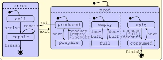
In this section, we define a model transformation from a variant of UML statecharts [OMG09] to Petri nets [Pet80] using triple rules and application conditions. Statecharts may have orthogonal regions as well as state nesting. As a small restriction, we do not handle entry and exit actions, do not allow extended state variables, allow guards only to be conditions over active states, and allow only a depth of two for hierarchies of states. For the target language of Petri nets, we use nets with inhibitor arcs, contextual arcs, and open places. A transition with an inhibitor arc from a place (denoted by a filled dot instead of an arrow head) is only enabled if there is no token on this place. A contextual arc between a place and a transition (denoted by an edge without arrow heads), also known as read arc in the literature, means that this token is required for firing, but remains on the place. Open places allow the interaction with the environment, i.e. token may appear or disappear without firing a transition within the net. We assume all places to be open. With these restrictions for statecharts and extensions for Petri nets we are able to define a model transformation from statecharts to Petri nets which preserves the semantical behavior, at least on an informal level.
error
call
repair
prod
produced
prepare
empty
full
wait
consumed
arrive
finish repair
finish exit
next produce[empty] /incbuff fail
inc-buff
dec-buff next
consume [full] /decbuff
Figure 1: The example statechart in concrete syntax In Figure 1, the
stat-echart ProdCons is de-picted modeling a producer-consumer system. The whole state machine con-tains one region with the states prod, error, and a final state. When initial-ized, the system is in the stateprod, which has three
regions. There, in parallel a producer, a buffer, and a consumer may act. The producer alternates between the statesproducedandprepare, where the transitionproducemodels the actual production activity. It is guarded by a condition that the parallel stateempty is also current, meaning that the buffer is empty and may actually receive a product, which is then modeled by the actionincbuffdenoted after the/-dash. Similarly to the producer, the buffer alternates between the statesemptyandfull, and the consumer betweenwaitandconsumed. The transitionconsume is again guarded by the statefull and followed by adecbuff-action emptying the buffer.
Two possible events may happen causing a state transition leaving the state prod: the con-sumer may decide to finish the complete run or there may be a failure detected after the produc-tion leading to theerror-state. Then, the machine has to be repaired before theerror-state can be exited via the correspondingexit-transition and the standard behavior in theprod-state is executed again.
SM name:String
R
E name:String
T
S name:String isInitial:Bool
isFinal:Bool A
name:String
G
R-T3
E-P
T-T
S-P
S-Pe
S-T1
S-T2
place
transition
pre inhibitor contextual post
region
regions states trigger
action guard begin
end
con-dition
sT G tT G
Figure 2: The triple type graphT G
InFigure 2, the triple type graphT Gis depicted, containing in the left the source component of statecharts in abstract syntax, in the right the target component of Petri nets, and the connection component inbetween. To obtain valid statechart models, some constraints are needed which are described in the following but are not shown explicitly.
Each diagram consists of exactly one state machineSMcontaining one or more regionsR. A region contains statesS, where state names are unique within one region. A state may again con-tain one or more regions. Each region is concon-tained in either exactly one state or the state machine. Moreover, states may be initial (attribute valueisInitial = true) or final (attribute value
isFinal=true), each region has to contain exactly one initial and at most one final state, and
final states cannot contain regions. A transitionTbegins and ends at a state, is triggered by an eventE, and may be restricted by a guardGand followed by an actionA. A guard has one or more states as conditions. There is a special event with attribute valuename="exit"which is reserved for exiting a state after the completion of all its orthogonal regions, which cannot have a guard condition. Moreover, final states cannot be the beginning of a transition and their name attribute has to be set toname="final". In addition, transitions cannot link states in different orthogonal regions, which means that both regions are directly contained in the same state.
The languageV LSC consists of all typed attributed graphs respecting the source component
T GSof the type graphT Gand the constraints as described above.
In the following, we present the triple rules that create simultaneously the statechart model, the connection part, and the corresponding Petri net. For simplicity, we depict the Petri nets in the target component in concrete syntax, while only writing node names in the connection component.
0 state0
state2
state1 1
2
T a
state4
state3 3
4 T
a a
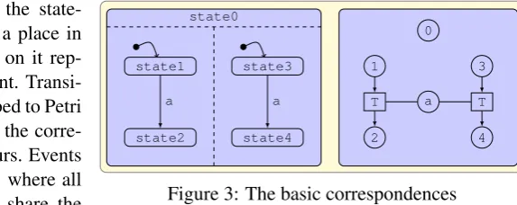
Figure 3: The basic correspondences In general, each state of the
state-chart model is connected to a place in the Petri net, where a token on it rep-resents that this state is current. Transi-tions between states are mapped to Petri net transitions and fire when the corre-sponding state transition occurs. Events are also connected to places, where all events with the same name share the
thus enabling the simultaneous firing of all enabled Petri net transitions when a token is placed there. By using contextual arcs it is possible that all transitions connected to an event with this name are enabled simultaneously if also their other pre-places are marked. Otherwise, we would not be able to fire all these transitions concurrently. They would not be independent but compete for the token. For independence, we had to know in advance how many of these transitions will fire to allocate that number of tokens on the event’s place. For a guard, the Petri net transition of its transition in the statechart diagram is the target of a contextual arc from the place connected to the condition. Thus, we check also in the Petri net that this guard condition is fulfilled, i.e. the corresponding place holds a token, before firing the transition. Such a basic situation is depicted inFigure 3, where altogether five states and their corresponding places, two transitions – both in the statechart and the Petri net – and an eventawith its corresponding place are shown. The hierarchy of the statechart is flattened, since Petri nets do not have such a concept. Note that all place are open places.
0 state0
state2
state1 1
2
T a
state4
state3 3
4 T
T2 T2
T2 T2
T3 T3
a a
0 state0
state1 1
f
T a
state3 3
f T T1
a a
Figure 4: The additional correspondences Additional places and
transi-tions make sure that the ef-fects of a state transition con-cerning involved sub- or super-states can be simulated also in the Petri net part. Each substate is connected via S-T2 to a T2 -transition which is the target of a pre-arc from its superstate. This makes sure that, when a state tran-sition leaves this superstate, also all substates are no longer cur-rent. Each region within a state is connected via R-T3 to a T3 -transition which makes sure that, when no state inside this region is
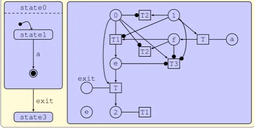
current, also the superstate is deactivated. These two situations are depicted in the example models in the top ofFigure 4. Each state that may contain regions is connected viaS-T1to a
T1-transition that is the target of pre-arcs from all places of final states and inhibitor arcs from all other places in its regions, while the superstate’s place is a contextual place as shown in the
state0
0
state1
1
2 T
a f
e
e exit
T T1
T1 T2
T2
T3
state3 a
exit
Figure 5: The handling ofexit-events bottom of Figure 4. This makes
-and T3-transitions. The idea behind this place is, that when all final states are reached and an exit transition has to be invoked, theT1-transition delivers a token to thee-place which than triggers the execution of the transition in the Petri net as shown inFigure 5.
For the operational semantics, all places in the Petri net corresponding to currently active states will be marked. Depending on the semantical steps in the statechart, the open places in the Petri net produce and delete tokens. For example, triggering an external event in the statechart leads to a token on the events’s place in the Petri net. Also for the handling of the hierarchical (de)activation the proper open places may fire triggered by the corresponding semantical rules for the statecharts. For example, when entering a state it’s initial substates become active. This has to be handled in the Petri net by firing the corresponding open places. Thus, the Petri net for itself shows different semantical behavior than the statechart, since arbitrary firing of open places leads to strange behavior, but every semantical step in the statechart can be simulated by the Petri net. The rules for the operational semantics of statecharts are given in [GBEE11].
start
L0,S ∅ L0∅,C L0∅,T
∅
R0,S R0,C R0,T ∅
SM name="sm"
ac0=¬∃p0
L0 ∅ ∅
SM name="sm"
tr0,S tr0,C tr0,T tL0
sL0
tR0
sR0
p0
Figure 6: The rulestart
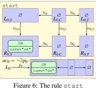
The start graph is the empty graph, and the first rule to be applied is the triple rulestartshown inFigure 6 which creates the start graph of statecharts in the source component, and empty connection and target compo-nents. The application conditionac0 is a so-called
neg-ative application condition (NAC) and forbids that the right hand side of the rule already exists before the rule is applied. Since a statemachine has exactly one nodeSM, the NAC ensures that the rule cannot be applied twice.
In Figure 7, the triple rules newRegionSM and
newRegionSare depicted which allow to create a new
region of a state machine or of a state, respectively. Since each region has to have an ini-tial state, this iniini-tial state is also created and connected to its corresponding place via S-P.
With newRegionSM, the initial state is also connected to a T1-transition in the target
com-ponent and another place viaS-Pe. Moreover, if the new region is created inside a state by
newRegionSthe substate is the inhibitor of the superstate’sT1-transition, the superstate
in-hibits a newT2-transition and the region and the substate inhibit a newT3-transition. For the triple rulenewRegionS, the application condition forbids that the superstate is final or already a substate of another state. newRegionSMhas the application condition true which is not de-picted. Note that we allow parameters for the rules to define the attributes. Thus, the user has to declare the name of the newly created state when applying these triple rules.
In Figs.8and9, the triple rules for creating new states are shown. WithnewStateSMand
newStateS, new states inside a region of the state machine or of a state are created, which are
not final states. Similarly, final states are created by the triple rulesnewFinalStateSMand
newFinalStateS. In all cases, a corresponding place is created in the target component. As
newRegionSM(sname:String)
L1,S L1,C L1,T
1:SM ∅ ∅
R1,S R1,C R1,T 1:SM
R
S name=sname isInitial=true
isFinal=false
e
T1
S-P S-Pe
S-T1
newRegionS(sname:String)
L2,S L2,C L2,T 1:S
S-P S-Pe S-T1
e
T1
R2,S R2,C R2,T 1:S
R
S name=sname isInitial=true
isFinal=false
e
T2
T3 T1
S-P S-Pe
S-P R-T3
S-T2 S-T1
ac2=¬∃p2∧ ¬∃q2
L2
1:S isFinal=true
S-P S-Pe S-T1
L2 S R 1:S
S-P S-Pe S-T1
p2
q2
sL1 tL1
sR1 tR1
tr1,S tr1,C tr1,T
sL2 tL2
sR2 tR2
tr2,S tr2,C tr2,T
Figure 7: The triple rulesnewRegionSMandnewRegionS
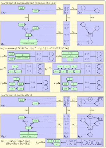
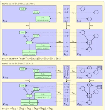
For the creation of a new transition, the triple rules newTransitionNewEvent,
newTransitionNewExit, newTransitionOldEvent, and
newTransitionOld-ExitinFigure 10andFigure 11are used. A new transition in the source part connected with a new Petri net transition in the target part is created, and in case of a new event, this event is connected with a new place which is a contextual place for the transition. Otherwise, the tran-sition is connected with the place of the already existing event. In case of anexit-event, the place connected viaS-Peto thebegin-state has to be connected to the new transition and the
begin-state’sT1-transition. The application conditions forbid that the begin-state is a final
newStateSM(sname:String)
L3,S L3,C L3,T 1:SM
2:R
∅ ∅
R3,S R3,C R3,T 1:SM
2:R
S name=sname isInitial=false
isFinal=false
T1
S-P
S-T1
e
S-Pe
ac3=¬∃p3 L3 1:SM 2:R S
name=sname ∅ ∅
newStateS(sname:String)
L4,S L4,C L4,T 1:S
2:R
S-P
R-T3
S-T1 T1
T3
R4,S R4,C R4,T 1:S
2:R
S name=sname isInitial=false
isFinal=false
T2
T3 T1
S-T1 S-P
S-P
S-T2 R-T3
ac4=¬∃p4 L4 1:S 2:R S name=sname
S-P
R-T3 S-T1
p3
p4
sL3 tL3
sR3 tR3
tr3,S tr3,C tr3,T
sL4 tL4
sR4 tR4
tr4,S tr4,C tr4,T
Figure 8: The triple rulesnewStateSMandnewStateS
thatexit-events only begin at superstates, i.e. a state containing a region. Note that the objects and morphisms used for the application conditionsac8,ac9, andac10 are not shown explicitly,
but they correspond to the objects and morphisms used inac7.
newFinalStateSM
L5,S L5,C L5,T 1:SM
2:R
∅ ∅
R5,S R5,C R5,T 1:SM
2:R
S name="final" isInitial=false
isFinal=true
S-P
ac5=¬∃p5 L5 1:SM 2:R
S
isFinal=true ∅ ∅
newFinalStateS
L6,S L6,C L6,T 1:S
2:R
S-T1 S-P R-T3
T1
T3
R6,S R6,C R6,T 1:S
2:R
S name="final" isInitial=false
isFinal=true
T1
T2 T3
S-T1
S-P S-P
R-T3
S-T2
ac6=¬∃p6 L6 1:S 2:R
S isFinal=true
S-T1 S-P R-T3
p5
p6
sL5 tL5
sR5 tR5
tr5,S tr5,C tr5,T
sL6 tL6
sR6 tR6
tr6,S tr6,C tr6,T
Figure 9: The triple rulesnewFinalStateSMandnewFinalStateS
An integrated model containing the statechart example in Figure 1 in its source component can be constructed by the application of the following triple rules:
1× startcreating the state machine,
1× newRegionSMcreating the one region inside the state machine and the initial stateprod,
1× newStateSMcreating the stateerror,
4× newRegionScreating one region withinerrorincluding the initial statecalland the
three regions withinprodincluding the initial statesproduced,empty, andwait,
4× newStateScreating the staterepairwithinerrorand the statesprepare,full,
newTransitionNewEvent(ename:String)
L7,S L7,C L7,T 1:S
2:S
S-P S-P
R7,S R7,C R7,T 1:S 2:S T E name=ename T S-P S-P E-P T-T
ac7=ename6=”exit”∧ ¬∃p7∧ ¬∃q7∧(∃r7∨ ∃s7∨ ∃t7∨ ∃u7)
L7 1:S 2:S E name=ename S-P S-P L7 2:S 1:S isFinal=true S-P S-P L7 R 1:S 2:S S-P S-P L7 R R R S S 1:S 2:S S-P S-P L7 R S 2:S R 1:S S-P S-P L7 R 1:S S R 2:S S-P S-P newTransitionNewExit
L8,S L8,C L8,T 1:S 2:S S-Pe S-T1 S-P S-P e T1
R8,S R8,C R8,T 1:S 2:S T E name="exit" T e T1 S-Pe S-T1 S-P S-P E-P T-T
ac8=¬∃p8∧ ¬∃q8∧ ∃v8∧ (∃r8∨ ∃s8∨ ∃t8∨ ∃u8) L8
1:S 2:S R
S-Pe S-T1
S-P
S-P e T1
begin end begin
end
sL7 tL7
sR7 tR7
tr7,S tr7,C tr7,T
p7 q7
r7 s7
v8
t7 u7
sL8 tL8
sR8 tR8
tr8,S tr8,C tr8,T
newTransitionOldEvent
L9,S L9,C L9,T 1:S
2:S
3:E name=ename
S-P
S-P
E-P
R9,S R9,C R9,T 1:S
2:S
T
E name=ename
3:E name=ename
T
S-P
S-P
E-P E-P T-T
ac9=ename6=”exit”∧ ¬∃q9∧(∃r9∨ ∃s9∨ ∃t9∨ ∃u9)
newTransitionOldExit
L10,S L10,C L10,T 1:S
2:S 3:E name="exit"
S-Pe S-T1 S-P S-P E-P
e T1
R10,S R10,C R10,T 1:S
2:S
T
E name="exit"
3:E
name="exit" T
e
T1
S-Pe S-T1 S-P S-P
E-P E-P T-T
ac10=¬∃q10∧(∃r10∨ ∃s10∨ ∃t10∨ ∃u10)∧ ∃v10
sL9 tL9
sR9 tR9
tr9,S tr9,C tr9,T
begin end
sL10 tL10
sR10 tR10
tr10,S tr10,C tr10,T
begin end
Figure 11:newTransitionOldEventandNewTransitionOldExit
1× newFinalStateSMcreating the final state of the state machine,
1× newFinalStateScreating the final state withinerror,
9× newTransitionNewEventcreating all transition except for theexit-transition
be-tweenerrorandprodand thenext-transition betweenconsumedandwait,
1× newTransitionExitcreating theexit-transition betweenerrorandprod,
2× newTransitionOldEventcreating thenext-transition betweenconsumedandwait
with the already known eventnext,
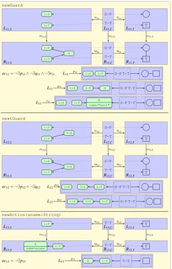
2× newGuardcreating the guards of theproduce- andconsume-transitions,
2× newActioncreating the actions of theproduce- andconsume-transitions.
newGuard
L11,S L11,C L11,T 1:S
2:T
S-P
T-T
T
R11,S R11,C R11,T 1:S
2:T
G
T
S-P
T-T
ac11=¬∃p11∧ ¬∃q11∧ ¬∃r11 L11 1:S 2:T S-P T-T
L11 1:S 2:T G S-P T-T
L11 1:S 2:T
E
name="exit" S-P T-T
nextGuard
L12,S L12,C L12,T 1:S
2:T
3:G
S-P
T-T
T
R12,S R12,C R12,T 1:S
2:T
3:G
T
S-P
T-T
ac12=¬∃p12∧ ¬∃q12
L12 1:S 3:G 2:T S-P T-T
L12 1:S 3:G 2:T S-P T-T
newAction(aname:String)
L13,S L13,C L13,T
1:T T-T T
R13,S R13,C R13,T 1:T
A
name=aname T
T-T
ac13=¬∃p13 L13 A 1:T T-T
sL12 tL12
sR12 tR12
tr12,S tr12,C tr12,T
q12
p12
sL11 tL11
sR11 tR11
tr11,S tr11,C tr11,T
p11
q11
r11
sL13 tL13
sR13 tR13
tr13,S tr13,C tr13,T
p13
produced
prepare
empty
f ull
wait
consumed next
produce
incbu f f
decbu f f
consume prod
f ail exit
error
call
repair
f inal
arrive
repair
e
error
e
prod
f inish
f inal
T
T
T
T
T
T
T2 T2 T2
T2 T2 T2
T1
prod
T T
T1
error
T2
T2
T2
T
T
T
T
T3 T3 T3
T3
Figure 13: The Petri net corresponding to the statechart inFigure 1
error
call
repair
prod
produced
prepare
empty
full
wait
consumed
arrive
finish repair
finish exit
next produce[empty] /incbuff fail
inc-buff
dec-buff next
consume [full] /decbuff
Figure 14: The statechart after the initialization step We do not want to show
the weak simulation relation between the statecharts se-mantics and the Petri net completely (see [Gol11]), but give some intuition how it works. First, the ini-tialization takes place. For the statechart, this leads to the active states prod,
produced,empty, and waitas shown inFigure 14with thicker lines, since the initial state
and all its initial substates are invoked. In the Petri nets, the corresponding open places create a token leading to the initial marking depicted inFigure 13.
de-activates the stateproducedand activates the stateprepare. In the Petri net, thenext-place generates a token. Now theT-transition withnext andproducedas pre-places is activated and fires. Since no other transition is activated, deleting the next-token leads to the result-ing Petri net simulation step with tokens on the places prod, prepare, empty, andwait
corresponding to the statechart’s current semantical state.
The source rules including suitable derived application conditions represent a generating grammar for our statechart models. All models are typed over the type graph and respect the specified constraints. For the target rules, only a subset of Petri nets can be generated, but all models obtained from transformations using the target rules are well-formed, because they are typed over the Petri net type graph and we cannot generate double arcs. This is due to the fact that the rules either create only arcs from or to a new element or the multiple application is forbidden as for the rulenewGuardby the expression¬∃p11within the application conditionac11.
4
Model Transformations with Application Conditions
As shown by the model transformation from statecharts to Petri nets, rules with application con-ditions are more expressive and allow to restrict the application of the rules. Thus, we enhance triple rules and combine a triple ruletrwithout application conditions with an application condi-tionacoverL. Then a triple transformation is applicable if the matchmsatisfies the application conditionac. From now on, a triple rule denotes a rule with application conditions, while the absence of application conditions is explicitly mentioned.
First, we introduce triple rules which construct the source, connection, and target parts in one step. From these triple rules we derive later the operational source and forward rules for the model transformation.
Definition 1 (Triple rule and transformation) A triple rule tr= (tr:L→R,ac) consists of triple graphsLandR, anM-morphismtr:L→R, and an application conditionacoverL.
Adirect triple transformation G===tr,m⇒Hof a triple graphGvia a triple ruletrand a matchm:
L→Gwithm|=acis given by the direct triple transformationG===tr,m⇒Hvia the corresponding triple rule without application conditions.
Example1 Examples for triple rules using application conditions have been shown inSection 3.
For the extension of the derived rules with application conditions, we need more specialized application conditions that can be assigned to the source and forward rules.
Definition 2 (Special application conditions) Given a triple ruletr:L→R, an application conditionac=∃(a,ac0)overLwitha:L→Pis an
• S-application conditionifaC, aT are identities, i.e. PC =LC, PT =LT, andac0 is anS -application condition overP, and
(LS LC LT)
(PS PC=LC PT =LT)
ac
ac0
S-application condition S-extending application condition
(LS LC LT)
(PS=LS PC PT)
ac
ac0
sL tL
sP tP=tL
aS idLC idLT
sL tL
sP tP
idLS aC aT
Moreover, true is anS- andS-extending application condition, and ifac,aciareS- orS-extending application conditions for some index setI so are¬ac,∧i∈Iaci, and∨i∈Iaci.
For the assignment of the application conditionacto the derived rules, the application condi-tion has to be consistent to the source and forward rules, which means that we must be able to decomposeacintoS- andS-extending application conditions.
Definition 3(S-consistent application condition) Given a triple ruletr= (tr:L→R,ac), then
acisS-consistentif it can be decomposed intoac∼=ac0S∧ac0F such thatac0Sis anS-application condition andac0F is anS-extending application condition.
CheckingS-consistency for arbitrary application conditions may be complex. Thus, we gen-erally assume that the designer of the triple rules specifies only conjunctions ofS-application conditions andS-extending application conditions. From the application point of view, this still provides sufficient expressive power. In fact, theS-application conditions allow for the specifi-cation of first order logic (FOL) expressions for the source component and theS-extending ones allow for FOL-expressions on the target component.
Example2 All triple rules inSection 3haveS-consistent application conditions. For example, the application conditionac7 of the rule newTransitionNewEvent in Figure 10is an S-application condition, thus no decomposition is necessary. Moreover, the S-application condition ac11 of the rulenewGuardinFigure 12can be decomposed into the S-application condition
¬∃q11∧ ¬∃r11and theS-extending application condition¬∃p11.
For anS-consistent application condition, we obtain the application conditions of the source and forward rules from theS- andS-extending parts of the application condition, respectively.
Definition 4(Derived rules with application conditions) Given a triple ruletr= (tr:L→R,ac)
withS-consistentac∼=ac0S∧ac0F we translateac0Sto an application conditionacS=toS(ac0s)on
(LS←∅→∅)andac0F to an application conditionacF=toF(ac0F)on(RS←LC→LT)using the constructions below. This leads to thesource rule(trS,acS)and theforward rule(trF,acF).
Given anS-application conditionac0Sand anS-extending application conditionac0F overL, we definetoS(ac0S)andtoF(ac0F)by
LS ∅ ∅
PS ∅ ∅
LS LC LT
PS PC=LC PT =LT toS(ac0S)
toS(ac00S) ac0S
ac00S
sL tL
sP tP=tL
idLS
aS id
LC idLT
aS
idPS
RS LC LT
RS PC PT LS LC LT
PS=LS PC PT toF(ac0F)
toF(ac00F) ac0F
ac00F
trS◦sL tL
sL tL
trS◦sP
tP
sP tP
trS idLC idLT
idLS aC aT
idRS aC aT
newGuardS
L11,S 1:S
2:T ∅ ∅
R11,S
1:S
2:T
G ∅ ∅
ac11,S=¬∃q11,S∧ ¬∃r11,S
L11,S 1:S
2:T G ∅ ∅
L11,S
1:S 2:T E name="exit"
∅ ∅
∅ ∅
∅ ∅
tr11,S ∅ ∅
q11,S
r11,S
newGuardF
R11,S L11,C L11,T 1:S
2:T 3:G
S-P
T-T
T
R11,S R11,C R11,T 1:S
2:T 3:G
T
S-P
T-T
ac11,F=¬∃p11,F
L11,F
1:S 2:T 3:G
S-P T-T
tr11,S◦sL11 tL11
sR11 tR11
idR11,S tr11,C tr11,T
p11,F
Figure 15: The source and forward rules ofnewGuard
• toS(true) =toF(true) =true,
• toS(∃(a,ac00S)) =∃((aS,id∅,id∅),toS(ac00S)), • toF(∃(a,ac00F)) =∃((idRS,aC,aT),toF(ac
00
F)), and • recursively for composed application conditions.
Example3 InFigure 15, the source and forward rulesnewGuardS andnewGuardF of the
rulenewGuardinFigure 12are shown. TheS-application condition¬∃p6∧ ¬∃r6is translated
to the source rule, where the source graphs of the original application conditions are kept, but the connection and target graphs are empty now. TheS-extending application condition¬∃q6is translated to the forward rule, where the source graph is adapted to the new left-hand side.
Similar to the corresponding result for triple rules without application conditions, in case of
S-consistency each triple rule is theE-concurrent rule of its source and forward rules.
Proposition 1 Given a triple rule tr= (tr:L→R,ac)with S-consistent ac, then tr=trS∗EtrF
with E being the domain of the forward rule.
Proof idea. From [EEE+07] we know that this holds for triple rules without application condi-tions. For the application conditions, this can be shown in two steps using the definition of the application conditions and the shift properties (see [Gol11]).
For the first step, we have to show that Shift((idLS,∅LC,∅LT),acS)∼=ac 0
S. WithacS=toS(ac0S) this is obviously true for ac0S =true. Consider ac0S =∃(a,ac00S) with a:L→ P and suppose Shift((idPS,∅LS,∅LC),toS(ac
00
S))∼=ac
00
S. It follows that Shift((idLS,∅LC,∅LT),toS(∃(a,ac 00
S)))∼= ∃(a,Shift((idPS,∅LS,∅LT),toS(ac
00
S))∼=∃(a,ac00S) =ac0S because the shift construction implies that only the trivial squares have to be considered for the index set.
For the second step, we have to show that L(e2,Shift(idE,acF))=∼ac0F with e2= (trS,idLC,
idLT):L→E. WithacF =toF(ac 0
F)this is obvious forac0F =true. ConsideracF0 =∃(a,ac00F) with L((LS ←PC →PT)→(RS←PC→ PT),Shift(id,toF(ac00F)))=∼ac00F. Then (PS =LS
sP
PC tP
→PT)is the pushout complement constructed for the left-shift-construction and we have that L(e2,Shift(idE,toF(∃(a,ac00F)))) =∼ L(e2,∃((idRS,aC,aT),toF(ac
00
F))) ∼= ∃((idLS,aC,aT),
L(((LS←PC→PT)→(RS←PC→PT)),toF(ac00F))∼=∃(a,ac00F) =ac0F.
Now we want to analyze how a triple transformation can be decomposed into a transformation applying first the source rules followed by the forward rules. Match consistency of the decom-posed transformation means that the comatches of the source rules define the source part of the matches of the forward rules. This helps us to define suitable forward model transformations, which have to be source consistent to ensure a valid model. Note, that triple transformation sequences always satisfy the application conditions of the corresponding rules.
Definition 5(Source and match consistency) Given a sequence(tri)i=1,...,nof triple rules with
S-consistent application conditions leading to corresponding sequences (triS)i=1,...,n and
(triF)i=1,...,nof source and forward rules. A triple transformation sequenceG00=
trS∗
=⇒Gn0=
trF∗
=⇒Gnn via firsttr1S, . . . ,trnSand thentr1F, . . . ,trnF with matchesmiSandmiFand comatchesniSandniF, respectively, ismatch consistentif the source component of the matchmiF is uniquely defined by the comatchniS.
A triple transformationGn0=
tr∗F
=⇒Gnnis calledsource consistentif there is a match consistent sequenceG00=tr
∗ S
=⇒Gn0=
tr∗F
=⇒Gnn.
We can split a transformationG0=
tr1
=⇒G1⇒. . .=
trn
=⇒Gninto transformationsG0=
tr1S
=⇒G00===tr1⇒F
G1⇒. . .=
trnS
=⇒G0n−1===trnF⇒Gn. But to apply first the source and then the forward rules, these have to be independent in a certain sense. In the following theorem, we show that such a decomposi-tion into a match consistent transformadecomposi-tion can be found and, vice versa, each match consistent transformation can be composed to a transformation via the corresponding triple rules if the application conditions areS-consistent. This result is an extension of the corresponding result for triple transformations without application conditions [EEE+07] and with negative applica-tion condiapplica-tions [EHS09]. It is essential for concepts and results of model transformaapplica-tions with application conditions below.
Theorem 1 (Decomposition and composition) For triple transformation sequences with S-consistent application conditions the following holds:
1. Decomposition:For each triple transformation sequence G0=tr=⇒1 G1⇒. . .=tr=⇒n Gnthere
is a corresponding match consistent triple transformation sequence G0=G00=
tr1S
=⇒G10⇒
. . .=tr=nS⇒Gn0===tr1F⇒Gn1⇒. . .===trnF⇒Gnn=Gn.
2. Composition:For each match consistent triple transformation sequence G00=
tr1S
=⇒G10⇒
. . .=tr=nS⇒ Gn0=
tr1F
==⇒ Gn1⇒. . .=
trnF
==⇒Gnn there is a triple transformation sequence G00= G0=tr=⇒1 G1⇒. . .=tr=⇒n Gn=Gnn.
3. Bijective Correspondence:Composition and Decomposition are inverse to each other.
transforma-tions viatriS andtrjF are sequentially independent fori> j. This is shown in [EEE+07] for rules without application conditions and can be extended to triple rules with application con-ditions as shown in the following. Thus, the proof from [EEE+07] can be done analogously for rules with application conditions. The main idea of the proof is that a triple transforma-tion sequence G0=tr1
=⇒ G1 ⇒. . .=trn
=⇒ Gn can be decomposed into a transformation sequence
G0=tr1S
=⇒ G01=tr1F
==⇒G1 ⇒. . .=trnS
=⇒ G0n=trnF
==⇒ Gn. The sequential independence oftriS andtrjF fori> jallows us to shift all source rules to the beginning and all forward rules to the end of the sequence leading to an equivalent transformation sequenceG0=G00=tr=1⇒S G10⇒. . .=tr=nS⇒ Gn0=
tr1F
==⇒Gn1⇒. . .=
trnF
==⇒Gnn=Gn.
It suffices to show that the transformationsG10=tr1F,m1
====⇒G11=tr2S,m2
===⇒G21are sequentially inde-pendent. From the sequential independence without application conditions we obtain morphisms
i:R1F →G11withi=n1and j:L2S→G10withg1◦j=m2.
It remains to show the compatibility with the application conditions:
• j|=ac2S: ac2S=toS(ac02S), where ac02S is anS-application condition. Forac02S=true, also ac2S=true and therefore j|=ac2S. Suppose ac02S=∃(a,ac
00
2S) leading to ac2S = ∃((aS,id∅,id∅),toS(ac
00
2S)). Moreover,tr1F is a forward rule, i. e. it does not change the source component andG11,S=G10,S.
L1F R1F
G10 G11
L2S R2S
G21
tr1F
g1
m1
i=n1
j
tr2S
g2
m2 n2
PS ∅ ∅
L2,S ∅ ∅
G10,S G10,C G10,T
G11,S=G10,S G11,C G11,T
toS(ac002S)
ac2S
sG10 tG10
sG11 tG11
aS
jS
id g1,C g1,T
pS
We know that m2=g1◦ j|=ac2S, which means that there exists p:P→G11 with p◦
a=g1◦ j, p|=toS(ac002S), and pC =∅, pT =∅. Then there exists q:P→G10 with q= (pS,∅,∅),q◦a= (pS◦aS,∅,∅) = j, andq|=toS(ac002S)because all objects occuring intoS(ac002S)have empty connection and target components. This means that j|=ac2Sfor this case, and can be shown recursively for composedac2S.
• g2◦n1|=acR :=R(tr1F,ac1F): ac1F =toF(ac01F), whereac01F is an S-extending appli-cation condition. For ac01F =true alsoac1F =true and acR =true, therefore g2◦n1|= acR. Now supposeac01F =∃(a,ac001F)leading toac1F =∃((idR1,S,aC,aT),toF(ac
00
1F))and
acR =∃((idR1S,bC,bT),ac
0
R) by component-wise pushout construction for the right-shift withac0R=R(u,toF(ac001F)). Moreover, tr2S is a source rule which means that g2,C and
g2,T are identities.
From the shift property of application conditions we know thatn1|=acRusing thatm1|= ac1F. This means that there is a morphism p:P→G11 with p◦a=n1, p|=ac0R, and
This means thatg2◦n1|=acR=∃(a,ac0R), and can be shown recursively for composed
acR.
R1,S L1,C L1,T
PS=R1,S PC PT
R1,S R1,C R1,T
PC0 =R1,S PC0 P
0
T tr1,S◦sL tL
sP tP
id aC aT
sR tR
sP0 tP0
id bC bT
id tr1,C tr1,T
id uC uT
PS0=R1,S PC0 PT0
R1,S R1,C R1,T
G11,S G11,C G11,T
G21,S G21,C=G11,C G21,T =G11,T
ac0R
acR
sP tP
sR tR
sG10 tG10
sG11 tG11
id bC bT
n1,S n1,C n1,T
g2,S id id
pS=n1,S pC pT
Based on source consistent forward transformations we define model transformations, where we assume that the start graph is the empty graph.
Definition 6(Model transformation) A(forward) model transformation sequence(GS,G0=
tr∗F
=⇒
Gn,GT) is given by a source graph GS, a target graph GT, and a source consistent forward
transformationG0=
tr∗F
=⇒GnwithG0= (GS←−∅ ∅−→∅ ∅)andGn,T=GT.
A(forward) model transformation MTF :V LSVV LTis defined by all (forward) model trans-formation sequences.
Definition 7(Model transformationSC2PN) For our triple transformations, the triple rules are given by the setT R={start,newRegionSM,newRegionS,newStateSM,newStateS,
newFinalStateSM, newFinalStateS, newTransitionNewEvent,
newTransi-tionNewExit, newTransitionOldEvent, newTransitionOldExit, newGuard,
nextGuard,newAction,newTriggerElement}as introduced inSection 3.
The model transformationSC2PNfrom statecharts to Petri nets is defined by all forward model transformations using the forward rulesT RF.
The source rules represent a generating grammar for our statechart models. Moreover, the restriction of all derived triple graphs to their source part, the language constructed by the source rules, and the statechart languageV LSC are equal.
Proposition 2(Comparison of statechart languages) Consider the languages V LS={GS | ∃
triple transformation∅=start===⇒=tr ∗
=⇒ (GS←GC→GT)via rules in T R}, V LS0={GS | ∃triple
transformation∅=startS ===⇒=tr
∗ S
=⇒(GS←∅→∅)via source rules in T RS}, and V LSC as defined
by the type graph and constraints. Then we have that V LS=V LS0=V LSC.
Proof idea. V LS ⊆V LS0: For a statechart GS∈V LS there is a transformation∅=start===⇒=tr ∗ =⇒
(GS←GC →GT) =Gn, which can be decomposed with Theorem 1into a corresponding
se-quence∅=start==⇒S =tr ∗ S
=⇒(GS←∅→∅) ====startF⇒=tr ∗ F
V LS0⊆V LSC: For a statechartGS∈V LS0there is a transformation∅=start==⇒S =tr ∗ S
=⇒(GS←∅→ ∅). GSis typed over the type graphT GSand respects all the specified constraints. This means thatGS∈V LSC.
V LSC⊆V LS: Given a statechart modelM∈V LSC we have to show that we find a transforma-tion sequence∅=start===⇒=tr
∗
=⇒GwithGS=M. We can show this by arguing about the composition ofMand how to select the corresponding triple rule creating each element inM in the source
part. This means thatM∈V LS.
Example4 As explained for our example transformation inSection 3, applying the correspond-ing source rule sequence to the empty start graph we obtain our statechart example. This state-chart model can be transformed into the Petri net via the forward rules. This triple transformation is source consistent, since the matches of the source parts for the forward rules are uniquely de-fined by the comatches of the source rules. Thus, we actually obtain a model transformation sequence from the statechart model inFigure 1to the Petri net inFigure 13.
For all notions and results concerning source and forward rules, we obtain the dual notions and results for target and backward rules. Thus, an application conditionacisT-consistent if it can be decomposed intoac∼=ac0T∧ac0B, whereac0T is aT-application condition with identities
aS,aC andac0B is aT-extending application condition with identityaT. This leads to target and backward rules with application conditions and the dual composition and decomposition prop-erties for triple transformation sequences withT-consistent application conditions. Moreover, a
backward model transformation sequence(GT,G00= tr∗B
=⇒G0n,GS)is based on a target consistent
backward transformationG00=tr ∗ B
=⇒G0nwithG00= (∅←−∅ ∅−→∅ GT)andG0n,S=GS.
4.1 Results for Model Transformations with Application Conditions
Based on Theorem 1we can show correctness, completeness, backward information preserva-tion, and termination of model transformations. The first result shows that transformations are correct and complete regarding the source and target languages.
Theorem 2(Correctness and completeness w.r.t. V LS,V LT) Each model transformation
se-quence(GS,G0=
trF∗
=⇒Gn,GT)and(GT,G00= trB∗
=⇒G0n,GS)is correct with respect to the source and
target languages, i.e. GS∈V LSand GT∈V LT.
For each GS∈V LS there is a corresponding GT ∈V LT such that there is a model
transfor-mation sequence(GS,G0=
tr∗F
=⇒Gn,GT). Similarly, for each GT ∈V LT there is a corresponding
GS∈V LSsuch that there is a model transformation sequence(GT,G00= trB∗
=⇒G0n,GS).
Proof. IfG0=
tr∗F
=⇒Gnis source consistent we have a match consistent sequence∅=tr ∗ S =⇒G0=
tr∗F
=⇒
Gn byDefinition 5. By composition in Theorem 1there is a triple transformation∅=tr ∗ =⇒Gn withGS=Gn,S∈V LSandGT∈V LT.
For GS ∈V LS there exists a triple transformation ∅=tr
∗
=⇒ G, which can be decomposed by
Theorem 1into a match consistent sequence ∅=tr ∗ S
=⇒ G0= (GS←−∅ ∅−→∅ ∅) =tr
∗ F
definition(GS,G0=
tr∗F
=⇒G,GT)is the required model transformation sequence withGT∈V LT. Dually, this holds for backward model transformation sequences.
Example 5 Since our example in Section 3 represents a well-defined model transformation sequence, our statechart and Petri net are correct. Moreover, for each valid statechart model we obtain a correct Petri net model, and vice versa. Note, that for the backward translation this only holds for Petri nets which are correct w.r.t. our target language, and not the language of all well-formed Petri nets.
A forward model transformation fromGStoGT is backward information preserving concern-ing the source component if there is a backward transformation sequence fromGT leading to the same source graphGS.
Definition 8(Backward information preserving) A forward transformation sequenceG=tr ∗ F
=⇒H
isbackward information preserving if for the triple graph H0 = (∅←−∅ ∅−→∅ HT)there is a backward transformation sequenceH0=tr
∗ B
=⇒G0withG0S=∼ GS.
This theorem is an extension of the corresponding result in [EEE+07] to triple transformations with application conditions.
Theorem 3(Backward information preservation) If all triple rules are S- and T -consistent, a
forward transformation G=tr ∗ F
=⇒H is backward information preserving if it is source consistent.
Proof. IfG=tr ∗ F
=⇒His a source consistent sequence then by Def.5there exists a match consistent sequence∅=
trS∗
=⇒G=tr ∗ F
=⇒Hleading to the triple transformation sequence∅=tr
∗
=⇒H using
Theo-rem 1. From the decomposition, we also obtain a match consistent sequence∅=tr ∗ T
=⇒H0=tr ∗ B
=⇒H
using the target and backward rules, withHT0 =HT andHC0 =HS0 =∅. Thus,G=tr ∗ F
=⇒His back-ward information preserving.
Example6 The Petri net inFigure 13can be transformed into the statechart inFigure 1using the backward rules of our model transformation in the same order as the forward rules were used for the forward transformation. Indeed, this holds for each Petri net obtained of a model transformation sequence from a valid statechart model.
If the source and target rules are creating, i.e. each rule actually creates at least one element, forward and backward transformation sequences are terminating. This means that we do not find infinite model transformation sequences.
Theorem 4(Termination) Consider a source model GS∈V LS (target model GT ∈V LT) and
a set of triple rules such that GS (GT) and all rule components are finite on the graph part and
the triple rules are creating on the source (target) component. Then each model transformation
sequence(GS,G0=
trF∗
=⇒Gn,GT)((GT,G00= tr∗B
=⇒G0n,GS)) is terminating, i.e. any extended sequence
G0=
tr∗F
=⇒Gn= tr0+F
==⇒Gm(G00= trB∗
=⇒G0n=tr 0+
B
Proof. LetG0=
tr∗F
=⇒ Gn be a source consistent forward sequence such that∅=tr ∗ S
=⇒G0=
tr∗F
=⇒Gn is match consistent, i.e. each comatchni,Sdetermines the source component of the matchmi,F. Thus, also each forward matchmi,F determines the corresponding comatchni,S. By uniqueness of pushout complements alongM-morphisms the comatchni,Sdetermines the matchmi,Sof the source step, thusmi,F determinesmi,S(∗).
If G0=tr ∗ F
=⇒ Gn=
tr(n+1,F),m(n+1,F)
=========⇒ Gn+1=
tr00∗F
==⇒ Gm is a source consistent forward sequence then
there is a corresponding source sequence∅=tr ∗ S
=⇒G0=tr===n+1,⇒S G00=tr 00∗
S
==⇒G0 leading to match
con-sistency of the complete sequence∅=⇒∗Gm. Using(∗)it follows thatG0∼=G0, which implies
that we have a transformation stepG0=
trn+1,S
===⇒ G00⊆G0, because triple rules are non-deleting.
This is a contradiction to the precondition that each rule is creating on the source component
implying thatG06∼=G0. Therefore, the forward transformation sequenceG0=
tr∗F
=⇒Gn cannot be extended and is terminating.
Dually, this can be shown for backward model transformation sequences.
Example7 All triple rules in our example inSection 3are finite on the graph part and source creating. Thus, all model transformation sequences based on finite statechart models are termi-nating. Note, that this does not hold for the backward direction, since the rulenewAction is not target creating. Thus, the corresponding backward rule can be applied infinitary often.
5
Conclusion
In this paper, we have extended the theory of model transformations based on TGGs to rules with nested application conditions [HP09], which are known to be equivalent to first order logic (FOL) on graphs. Using the slight restriction to S-consistent application conditions we have shown that the main results known for model transformations are preserved. In fact, this is a substantial extension of the existing theory, becauseS-consistent application conditions provide the expressive power of FOL separately for the source and target components of triple graphs, respectively. This enhances the expressiveness of model transformations including that of the generation of source and/or target languages. We have discussed in detail a model transformation from statecharts to Petri nets, where the use of application conditions allows to specify and translate more general statecharts then those considered in [EEPT06]. There, an inplace model transformation is used, which means that the model itself is changed in contrast to our approach, where the original source model is kept and an additional target model is created. We have presented main results for termination, correctness, completeness, and information preservation extending those for the case with NACs in [EHS09] and without NACs in [EEE+07].
Our new results are based on the Local Church–Rosser, Parallelism, and Concurrency Theo-rems with nested application conditions in [EHL10]. As future work it remains to extend also the results concerning functional behaviour in [HEOG10] and [HEGO10] to the case of rules with nested application conditions based on the “on-the-fly construction” in [EEHP09]. This would allow to meet the “Grand Research Challenge of the TGG Community” in [SK08] for our enhanced framework.
Petri nets is semantically correct, where the semantics of the source and target language could be based on a suitable operational semantics. For statecharts, an operational semantics based on amalgamated graph transformation is presented in [GBEE11]. In [Gol11], also an operational semantics for Petri nets using amalgamated graph transformation is defined and the model trans-formation given in this paper is shown to be semantics-preserving. It is future work to obtain general criteria for semantical correctness of model transformations.
Another future point of work is the construction of source and forward application conditions for general, not necessarilys-consistent application conditions. Obviously, in this case a different property for the compatibility of the source and forward solutions would be required to ensure the corresponding decomposition and composition result.
Bibliography
[EEE+07] H. Ehrig, K. Ehrig, C. Ermel, F. Hermann, G. Taentzer. Information Preserving Bidi-rectional Model Transformations. In Dwyer and Lopes (eds.),Proceedings of FASE 2007. LNCS 4422, pp. 72–86. Springer, 2007.
[EEH08] H. Ehrig, C. Ermel, F. Hermann. On the Relationship of Model Transformations Based on Triple and Plain Graph Grammars. In Karsai and Taentzer (eds.), Pro-ceedings of GraMoT 2008. Pp. 9–16. ACM, 2008.
[EEHP09] H. Ehrig, C. Ermel, F. Hermann, U. Prange. On-the-Fly Construction, Correctness and Completeness of Model Transformations Based on Triple Graph Grammars. In Sch¨urr and Selic (eds.),Proceedings of MODELS 2009. LNCS 5795, pp. 241–255. Springer, 2009.
[EEPT06] H. Ehrig, K. Ehrig, U. Prange, G. Taentzer.Fundamentals of Algebraic Graph Trans-formation. EATCS Monographs. Springer, 2006.
[EHL10] H. Ehrig, A. Habel, L. Lambers. Parallelism and Concurrency Theorems for Rules with Nested Application Conditions.ECEASST 26:1–23, 2010.
[EHS09] H. Ehrig, F. Hermann, C. Sartorius. Completeness and Correctness of Model Trans-formations based on Triple Graph Grammars with Negative Application Conditions.
ECEASST 18:1–18, 2009.
[GBEE11] U. Golas, E. Biermann, H. Ehrig, C. Ermel. A Visual Interpreter Semantics for Stat-echarts Based on Amalgamated Graph Transformation.ECEASST 39:1–24, 2011. This volume.
[GL06a] E. Guerra, J. de Lara. Attributed Typed Triple Graph Transformation with Inher-itance in the Double Pushout Approach. Technical report UC3M-TR-CS-2006-00, Universidad Carlos III, Madrid, Spain, 2006.
[Gol11] U. Golas.Analysis and Correctness of Algebraic Graph and Model Transformations. PhD thesis, Technische Universit¨at Berlin, Vieweg + Teubner, 2011.
[HEGO10] F. Hermann, H. Ehrig, U. Golas, F. Orejas. Efficient Analysis and Execution of Correct and Complete Model Transformations Based on Triple Graph Grammars. In B´ezivin et al. (eds.),Proceedings of MDI 2010. Pp. 22–31. ACM, 2010.
[HEOG10] F. Hermann, H. Ehrig, F. Orejas, U. Golas. Formal Analysis of Functional Behaviour for Model Transformations Based on Triple Graph Grammars. In Proceedings of ICGT 2010. LNCS 6372, pp. 155–170. Springer, 2010.
[HP09] A. Habel, K.-H. Pennemann. Correctness of High-Level Transformation Systems Relative to Nested Conditions.MSCS19(2):245–296, 2009.
[KS06] A. K¨onig, A. Sch¨urr. Tool Integration with Triple Graph Grammars - A Survey.
ENTCS148(1):113–150, 2006.
[OMG09] OMG. Unified Modeling Language, Superstructure, Version 2.2. 2009.
[Pet80] C. Petri. Introduction to General Net Theory. In Brauer (ed.),Net Theory and Appli-cations. LNCS 84, pp. 1–19. Springer, 1980.
[Sch94] A. Sch¨urr. Specification of Graph Translators With Triple Graph Grammars. In Tin-hofer (ed.),Proceedings of WG 1994. LNCS 903, pp. 151–163. Springer, 1994.
[SK08] A. Sch¨urr, F. Klar. 15 Years of Triple Graph Grammars. In Ehrig et al. (eds.), Pro-ceedings of ICGT 2008. LNCS, pp. 411–425. Springer, 2008.
[TEG+05] G. Taentzer, K. Ehrig, E. Guerra, J. Lara, L. Lengyel, T. Levendovsky, U. Prange, D. Varr´o, S. Varr´o-Gyapay. Model Transformation by Graph Transformation: A Comparative Study. In Proceedings of MTP 2005. 2005.