Hungarian Association of Agricultural Informatics European Federation for Information Technology in Agriculture, Food and the Environment
Journal of Agricultural Informatics. Vol. 9, No. 2 journal.magisz.org
Modeling the effect of olive fruit bearing percentage on Bactrocera oleae
stochastic dispersion*
Romanos Kalamatianos
1, Pavlos Bouchagier
2, Markos Avlonitis
3I N F O
Received 16 Feb 2018 Accepted 9 Jun 2018 Available on-line 18 Jun 2018 Responsible Editor: M. Herdon
Keywords:
olive fruit fly, dispersion, simulation, olive fruit bearing
A B S T R A C T
Olive fruit fly’s dispersion depends upon the olive fruit bearing percentage inside the olive grove. Previous efforts to simulate the dispersion based on the olive fruit percentage produced promising results. However the effect of olive fruit fly’s percentage and fruit fly dispersion in space were not modelled correctly in some cases. In this work we improved the dispersion model to map the data obtained better. Simulated data were compared with the measured data by computing three metric indexes. For the case of 0% olive fruit the simulated data were nearly identical to the measured data, while for the case of 30% olive fruit the reproduction of the measured data was quite promising.
1. Introduction
Olive fruit fly is a parasitic insect that infests olive groves as the development of the pre-imaginal stages (egg, larva, pupa) is solely dependent on the presence of olive fruits. Therefore, if left unchecked the olive fruit fly can cause great damage in both quality and quantity of the crop (Rice 2000; Neuenschwander & Michelakis 1978). Due to its dependence on olive fruits for its reproduction it seems logical that dispersion of the adult population of the insect would be dependent from the presence of olive fruit inside the olive grove. In their experiments, Fletcher & Kapatos (1981) showed that as the percentage of olive fruit presence decreases the olive fruit fly travels longer distances. Specifically, when olive fruit flies were released in an olive grove with 30% of olive fruit production the olive fruit flies traveled an average distance of 180m in one week. However, when released in an olive grove with 0% olive fruit (no olive fruit production) the olive fruit flies traveled an average distance of over 450m in one week.
Moreover the population evolution of the olive fruit fly depends upon climate parameters (Broufas, Pappas & Koveos 2009; Johnson et al 2011; Pappas et al 2011; Tsitsipis 1977; Tsitsipis 1980; Tsitsipis & Abatzis 1980). However, other factors play also an essential role, such as the spatiotemporal evolution of the olive fruit fly’s population. A model for the population evolution of the olive fruit fly incorporating the spatial dispersion of the fly was introduced by Avlonitis, Tragoudaras & Stefanidakis (2007). This was accomplished by the stochastic generalization of the logistic equation, with arbitrary initial and boundary conditions for the olive fruit fly population.
(1) 𝜕𝜕𝜕𝜕𝜕𝜕𝜕𝜕=𝛽𝛽𝛽𝛽(1− 𝛽𝛽) +𝑐𝑐𝜕𝜕𝑥𝑥𝜕𝜕2𝜕𝜕2+𝑔𝑔(𝛽𝛽)𝛿𝛿𝛽𝛽
where p is the population density, is the rate of increase, 𝑐𝑐𝜕𝜕2𝜕𝜕
𝜕𝜕𝑥𝑥2 is the diffusion term in space and g(p)p
models the spatiotemporal stochasticity and g(p) being the corresponding noise amplitude.
1 Romanos Kalamatianos
Department of Informatics, Ionian University
[email protected] 2 Pavlos Bouchagier
Department of Food Technology, Technological Educational Institute of Ionian Islands
[email protected] 3 Markos Avlonitis
Department of Informatics, Ionian University
Voulgaris et al (2013) introduced a simulation model that estimates olive fruit fly population outbreaks, with the intent to be used as a real-time alert system. Outbreaks’ estimation is achieved by providing input information about olive grove location, trap data collected from the field, along with environmental data. Through their experiments, Voulgaris et al (2013) established that predicting the time when a population outbreak will occur, could help to estimate the proper time to apply population control methods.
The aforementioned model was upgraded by Kalamatianos, Avlonitis & Stravoravdis (2015) by making the dispersion model of the olive fruit fly temperature dependent, in the sense that, when temperature exceeds a predefined threshold, olive fruit flies are motionless. Furthermore, they modified the time of immature stages of the olive fruit fly, needed to complete development. The time taken for each olive fruit fly to develop from an egg to a fully grown adult became more random instead of a fixed time which was the case in the model proposed by Voulgaris et al (2013). The simulation scenarios conducted by Kalamatianos, Avlonitis & Stravoravdis (2015), revealed how the level of infestation is affected under diverse temperature sets and drifting distances in addition to the number of starting areas the initial population emerged.
Kalamatianos & Avlonitis (2015) further upgraded the aforementioned model (Kalamatianos, Avlonitis & Stravoravdis 2015) by changing the time resolution of the simulation from days to hours. Furthermore, based upon field measurements (Fletcher & Kapatos 1981), they improved the dispersion model of the olive fruit fly based on the olive fruit’s percentage in the olive grove. In this work olive fruits percentage and symmetric spatial distribution of the olive fruit fly population were not modeled in detail. While for 0% olive fruit the average traveled distance was correctly reproduced, this was not the case for the 30% of olive fruit, as it was shown by Fletcher & Kapatos (1981).
In this paper, we further improve the dispersion model in order to address the aforementioned issues and to better reproduce the findings from the experiments that were conducted by Fletcher & Kapatos (1981). We compare our results with the field measurements by Fletcher & Kapatos (1981) and use three metric indexes to validate the simulated data. We also compare our model against a field experiment conducted by Rempoulakis & Nestel (2012), in which, although olive fruit fly dispersion in relation to the presence of olive fruit was not the main focus of the experiment, it is derived that for 40% olive fruit, olive fruit flies traveled in average 46.5m three days after their release.
2. Material and Methods
2.1. Simulation Model
In this subsection, we describe the simulation model, implemented with the Python programming language, employed for our experiments.
1) Input data
For a simulation the following input data must be supplied. First, the field on which the simulation will take place must be given. The information required, is the field dimensions, the location of olive groves and the olive fruit percentage of each olive grove. Following, the climate of the field must be given, namely the temperature of the field. Although, the development and activity of the olive fruit fly depends also on more environmental parameters, such as relative humidity (Broufas, Pappas & Koveos 2009; Tsitsipis & Abatzis 1980) currently only temperature is incorporated into the simulation model. The total number of temperature values must be equal to the total number of simulation steps. In addition, the total olive fruit flies present at the start of the simulation and their position inside the field are required. Finally, the total number of simulation steps must be given.
2) Population structure
We structured the population of the olive fruit fly into the following transformation stages:
1. Egg.
3. Pupa.
4. Immature adult. We consider all adults with undeveloped ovaries as immature.
5. Mature adult.
6. Dead.
The first three transformation stages are considered as the immobile population of the olive fruit fly, since they do not move until the adult fly emerges. When an olive fruit fly reaches its fourth transformation stage it is able to drift on the field.
3) Development
The time resolution used by the model is hourly, which means that one simulation step corresponds to one hour following the methodology by Kalamatianos & Avlonitis (2015). In order to accurately model the development of the olive fruit fly, we utilized the Degree Day model (Wilson & Barnett 1983). Various methods have been proposed to calculate Degree Day units (Wilson & Barnett 1983; Brown 2013) however, we use the method shown in Equation (2), introduced by Voulgaris et al (2013) and slightly modified by Kalamatianos & Avlonitis (2015), to calculate the accumulated degree hour units of each fly.
(2) 𝐷𝐷𝐷𝐷=(𝜕𝜕𝑖𝑖−𝑇𝑇𝐿𝐿)�1−
1 1+𝑒𝑒−10�𝑡𝑡𝑖𝑖−𝑇𝑇𝑈𝑈��
24
where ti is the temperature in the i-th simulation step, TL and TU are the lower and upper
developmental thresholds, respectively, of each olive fruit fly. When an olive fruit fly reaches its Degree Day threshold it transforms to the succeeding transformation stage.
3) Oviposition
The model assumes that all olive fruit flies are females and thus can lay eggs, only when they reach the mature adult transformation stage. Each olive fruit fly can lay up to three eggs in its lifespan, up to one egg per day and exclusively during daytime hours (Johnson et al 2011; Avidov 1954). The total number of eggs was selected to account for mortality.
4) Dispersion
The speed at which an olive fruit fly drifts inside the simulated field depends on two parameters, namely, the temperature and the olive fruits’ percentage. The average speed of an olive fruit fly based on the olive fruits’ percentage of its current position was calculated with Equation (3) (Kalamatianos & Avlonitis (2015),
(3) 𝐴𝐴𝐴𝐴𝑔𝑔𝐴𝐴𝛽𝛽𝐴𝐴𝐴𝐴𝐴𝐴�𝑓𝑓𝑥𝑥,𝑦𝑦�=451.8∗𝑒𝑒
−0.04098∗𝑓𝑓𝑥𝑥,𝑦𝑦
𝑤𝑤ℎ
where fx,y is the olive fruit percentage on (x,y) coordinates of the grid and wh the total daytime hours
in the current week.
We observed, however, that for an olive fruit percentage of 30% the dispersion model couldn't reproduce the field measurements, for the same fruit percentage, as in Fletcher & Kapatos (1981). Therefore, we modified Equation (3) from the exponential to a linear Equation (4), as shown in Figure 1, still based on the assumption that for 100% olive fruit the olive fruit fly has no preferred direction. Thus, the emerging equation is as follows:
Figure 1. Curves for the mean travelled distance of olive fruit flies. Curve (a) exponential law proposed by Kalamatianos & Avlonitis (2015) curve (b) linear law proposed in this work.
The final speed is calculated by Equation (5) based on the temperature at its current position (Kalamatianos, Avlonitis & Stravoravdis, 2015).
(5) 𝐴𝐴𝛽𝛽𝐴𝐴𝐴𝐴𝐴𝐴=𝐴𝐴𝐴𝐴𝑔𝑔𝐴𝐴𝛽𝛽𝐴𝐴𝐴𝐴𝐴𝐴�𝑓𝑓𝑥𝑥,𝑦𝑦� ∗ �1− 1+𝑒𝑒−10∗�𝑡𝑡𝑖𝑖−𝑇𝑇𝑀𝑀�1 �
where ti is the temperature present in the i-th simulation step, TM is the upper movement threshold.
The upper movement threshold was set to 35 oC while beyond this temperature the olive fruit flies stop
drifting (Johnson et al 2011; Avidov 1954). Instead of the modified random walker model used by Kalamatianos & Avlonitis (2015), we employ alternative method for the movement of the olive fruit flies inside the grid. Specifically, each adult olive fruit fly that emerges picks a random direction to move towards. At each time step it has three choices either it continues to move towards the same direction, or it moves towards the opposite direction or it doesn't move. Each choice has a probability which changes based on the olive fruit percentage of the current position of the olive fruit fly (see Figure 2). For 100% olive fruit all choices are equiprobably.
Figure 2. Probability to choose a direction state based on olive fruit percentage.
2.2. Simulation Scenarios
scenario the time period was set to three days or 72 simulation steps. The diurnal day/night cycle was set to 14 and 10 hours respectively. Thus, dispersion was possible in only 98 (14h daytime x 7 days) time steps for the first two simulation scenarios and 42 (14h daytime x 3 days) time steps for the last. Since, dispersion in relation to the presence of olive fruit was the main focus of the simulations, the temperature assumed was constant, namely 27oC, at all simulation steps and below the temperature
movement threshold. The variable that was changed in each scenario was the olive fruit percentage, which was set to 0%, 30% and 40% respectively. Each simulation scenario was executed 100 times.
3. Results and Discussion
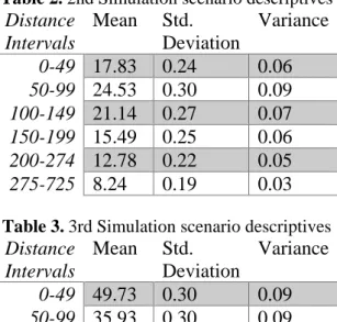
In this Section the results of the execution of the three simulation scenarios are presented. Table 1 - 3, all metrics were calculated with the PSPP statistical analysis software, present the results after 100 executions of all scenarios, respectively. In addition, the simulation results are compared against the measured data for validation purposes.
Table 1.1st Simulation scenario descriptives
Distance
Intervals
Mean
Std.
Deviation
Variance
0-49
0.59
0.05
0.00
50-99
1.73
0.09
0.01
100-149
2.92
0.11
0.01
150-199
4.09
0.12
0.01
200-274
8.45
0.19
0.04
275-725
82.23
0.25
0.06
Table 2.2nd Simulation scenario descriptives
Distance
Intervals
Mean
Std.
Deviation
Variance
0-49
17.83
0.24
0.06
50-99
24.53
0.30
0.09
100-149
21.14
0.27
0.07
150-199
15.49
0.25
0.06
200-274
12.78
0.22
0.05
275-725
8.24
0.19
0.03
Table 3.3rd Simulation scenario descriptives
Distance
Intervals
Mean
Std.
Deviation
Variance
0-49
49.73
0.30
0.09
50-99
35.93
0.30
0.09
100-149
14.34
0.23
0.05
150-199
0
0
0
200-274
0
0
0
275-725
0
0
0
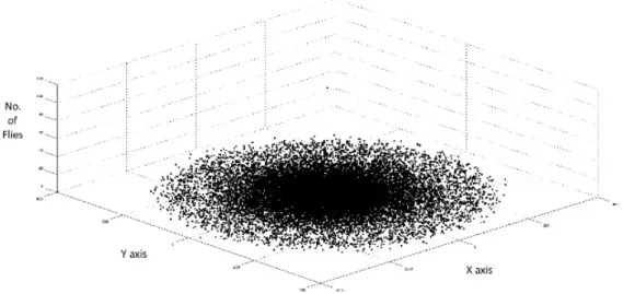
Figure 3. Spatial distribution of olive fruit flies for 0% olive fruits’ presence in olive grove for a time period of one week.
Figure 4 displays the relative frequency, in percentage, of olive fruit flies at specified distance intervals after the end of the first simulation scenario. The simulated data are compared to the observed data from Fletcher & Kapatos (1981) for 0% olive fruit presence. When there is no olive fruit present in the olive grove, over 80% of the olive fruit flies have traveled a distance of at least 275m from their starting position while for distances smaller than 275m smaller percentages of olive fruit flies can be found.
Figure 4. Relative frequency of olive fruit flies compared to observed data from Fletcher & Kapatos
(1981) for 0% olive fruit presence for a time period of one week.
When compared to the observed data from Fletcher & Kapatos (1981), it seems that the simulation model reproduced the observed data quite well. Indeed, olive fruit fly presence gets more frequent as the distance from the starting position increases, while the same behavior can be seen in the observed data. A quantitative comparison of simulated and real data correlation will be given below (see Table 4).
Figure 5. Spatial distribution of olive fruit flies for 30% olive fruit presence in olive grove for a time period of one week.
Figure 6 displays the relative frequency, in percentage, of olive fruit flies at specified distance intervals after the end of the second simulation scenario. The simulated data are, again, compared to the observed data from Fletcher & Kapatos (1981) for 30% olive fruit presence. The simulated data reproduce the behavior of the observed data although there are large fluctuations between the two data sets at each distance interval.
Figure 6. Relative frequency of olive fruit flies compared to observed data from Fletcher & Kapatos
(1981) for 30% olive fruit presence for a time period of one week.
Figure 7. Average flight distance of olive fruit flies compared to observed data from Rempoulakis & Nestel (2012), for 40% olive fruit presence for a time period of three days.
To validate the dispersion model a comparison between the simulated data against the measured data from Fletcher & Kapatos (1981) was done, specifically a comparison between the relative frequencies in relation to specified distance intervals was made. The following indices, which were also used by Yang et al (2013), were used to estimate the closeness of the datasets: correlation coefficient (R), Bias (Koboyashi & Salam 2000) and root mean square error (RMSE). When the values of the two latter indices are close to zero, this indicates that the datasets are close to each other. All aforementioned indices were computed via a script in the Python programming language.
𝐵𝐵𝐵𝐵𝐵𝐵𝐵𝐵=𝑁𝑁1×� 𝑂𝑂𝐵𝐵𝐴𝐴𝑖𝑖− 𝐴𝐴𝑆𝑆𝑆𝑆𝑖𝑖
𝑅𝑅𝑆𝑆𝐴𝐴𝑅𝑅=�∑𝑁𝑁𝑖𝑖=1(𝑂𝑂𝐵𝐵𝐴𝐴𝑁𝑁𝑖𝑖− 𝐴𝐴𝑆𝑆𝑆𝑆𝑖𝑖)2
OBSi and SIMi are the measured and simulated value, respectively, of the ith data point in N
observations.
The dispersion model validation was done for the cases of 0% and 30% olive fruit, since only for those two cases the measured data were available. Additionally, for the case of 30% olive fruit, Fletcher & Kapatos (1981) measured for the distance interval of 150-199m, no appearance of olive fruit flies, which we consider as an outlier due, for example, to trap malfunction. Therefore, we computed the aforementioned indices once for the whole dataset and once by merging the measurements for the distance interval of 150-199m with the measurements of the distance interval 200-274m. The detailed results are displayed in Table 4.
Table 4.Validation indices values
Fruit
percentage
Validation indices
R
Bias
RMSE
0%
0.9980 1.38167
1.931
30%
0.595
6.771667 8.272802
30%*
0.775
4.438
4.999998
* merging 150 – 199m and 200-274m
cases
measured values. However, for 30% olive fruit presence the following results were computed: 0.595, 6.771667 and 8.272802 respectively, which indicates that the estimated relative frequencies have a low correlation with the measured values. On the other hand, when we merged the distance intervals 150-199m and 200-274m, for the case of 30% olive fruit presence, the following results were computed: 0.775, 4.438 and 4.999998 respectively. By merging the aforementioned cases the estimated relative frequencies have a stronger correlation with the measured values, for this specific case.
4. Conclusion
We improved the dispersion model proposed by Kalamatianos & Avlonitis (2015) in order to better reproduce the results from the experiments conducted in Fletcher & Kapatos (1981). We validated our simulated data using the following three indexes: correlation coefficient (R), Bias (Koboyashi & Salam, 2000) and root mean square error (RMSE).
Simulation results showed, when compared to the results of Fletcher & Kapatos (1981) that for 0% olive fruit the relative frequency of olive fruit flies at specified distance intervals increases as we move further away from the origin point, which was observed as well in the field measurements, as well. Additionally, small fluctuations from the measured data were observed. When, the three metric indexes were computed they revealed a strong closeness and correlation between the simulated and measured data. For the case of 30% olive fruit presence the relative frequency of olive fruit flies at specified distance intervals have a similar tendency as the field measurements although there are large fluctuations between them. The computed values of the three metric indexes showed that there are not that strongly correlated as was the case of 0% olive fruit. Finally, when we merged, in our comparison, the values of the distance intervals 150-199m and 200-274m for the case of 30% olive fruit, since we considered that the field measurement for the 150-199m interval was a coincidence, the values of the metric indexes improved.
When compared to the results of Rempoulakis & Nestel (2012) we found that we were 9m off in regard to the average distance traveled by the olive fruit flies after three days. However, we consider this difference not too large, since in the field 5m could correspond to the distance between two olive trees.
We conclude that the proposed improvement of the olive fruit fly dispersion model, based on the comparison between the simulated and measured data, reproduced the field measurements sufficiently, especially for the case of 0% olive fruit.
Acknowledgment
The financial support of the European Union and Greece (Partnership Agreement for the Development Framework 2020) under the Regional Operational Programme Ionian Islands 2014-2020, for the project “Olive Observer” is gratefully acknowledged.
References
Avidov, Z 1954, ‘Further investigations on the ecology of the olive fly (dacus oleae, gmel.) in israel’. Ktavim, vol. 4, pp. 39-50.
Avlonitis, M, Tragoudaras D & Stefanidakis, M 2007, ‘Stochastic processes and insect outbreak systems: Application to the olive fruit fly’. Proceedings of the 3rd IASME/WSEAS International Conference on energy, environment, ecosystems and sustainable development, pp. 98-103.
Broufas, G, Pappas, M & Koveos D 2009, ‘Effect of relative humidity on longevity, ovarian maturation, and egg production in the olive fruit fly (Diptera: Tephritidae)’. Entomologia Experimentalis et Applicata, vol. 55, pp. 161-168. https://doi.org/10.1111/j.1570-7458.1990.tb01359.x
Brown, PW 2013, ‘Heat units’. Cooperative Extension Service, University of Arizona, Tucson, Arizona. Miscell Publ.
Fletcher, BS & Kapatos, E 1981, ‘Dispersal of the olive fly, dacus oleae, during the summer period on corfu‘.Entomologia Experimentalis et Applicata, vol. 29, pp. 1-8.
Johnson, M, Wang, X, Nadel, H, Opp, S, Lynn-Paterson, K, Stewart- Leslie J & Daane, K 2011, ‘High temperature affects olive fruit fly populations in californias central valley’. California Agriculture, vol. 65, pp. 29-33. https://doi.org/10.3733/ca.v065n01p29
Kalamatianos, R & Avlonitis, M 2015, ‘The role of tree distribution and olive fruit bearing in olive fruit fly infestation’. Proceedings of the 7th International Conference on Information and Communication Technologies in Agriculture, Food and Environment, Vol. 1498, CEUR Workshop Proceedings, pp. 720-729.
Kalamatianos, R, Avlonitis M & Stravoravdis, S 2015, ‘Complex networks and simulation strategies: An application to olive fruit fly dispersion’. Proceedings of the 6th International Conference on Information, Intelligence, Systems and Applications (IISA), IEEE. https://doi.org/10.1109/IISA.2015.7388025
Neuenschwander, P & Michelakis, S 1978, ‘Infestation of dacus oleae (gmel.) (diptera, tephritidae) at harvest time and its influence on yield and quality of olive oil in crete’. Journal of Applied Entomology, vol. 86, pp. 420-433. https://doi.org/10.1111/j.1439-0418.1978.tb01948.x
Pappas, ML, Broufas, GD, Koufali, N, Pieri P & Koveos, DS 2011, ‘Effect of heat stress on survival and reproduction of the olive fruit fly Bactocera (Dacus) oleae’. Journal Applied Entomology, vol. 135, pp. 359–366.
https://doi.org/10.1111/j.1439-0418.2010.01579.x
Rempoulakis, P. & Nestel, D 2012, Dispersal ability of marked, irradiated olive fruit flies [Bactrocera oleae (Rossi) (Diptera: Tephritidae)] in arid regions. Journal of applied entomology, vol. 136, no. 3, pp. 171-180.
https://doi.org/10.1111/j.1439-0418.2011.01623.x
Rice, R 2000, ‘Bionomics of the olive fruit fly bactrocera (dacus) oleae’. University of California Plant Protection Quarterly, vol. 10, pp. 1-5.
Tsitsipis, JA 1977, ‘Effect of constant temperatures on eggs of olive fruit fly, Dacus oleae (Diptera: Tephritidae) ’. Ann. Zool. Ecol. Anim, vol. 9, pp. 133–140.
Tsitsipis, JA 1980, ‘Effect of constant temperatures on larval and pupal development of olive fruit flies reared on artificial diet’. Environmental Entomology, vol. 9, no.6, pp. 764–68. https://doi.org/10.1093/ee/9.6.764
Tsitsipis JA & Abatzis, C 1980, ‘Relative humidity effects, at 20, on eggs of the olive fruit fly, Dacus oleae (Diptera Tephritidae), reared on artificial diet’. Entomologia Experimentalis et Applicata, vol. 28, pp. 92–99.
https://doi.org/10.1007/BF00422028
Voulgaris, S, Stefanidakis, M, Floros A & Avlonitis, M 2013, ‘Stochastic modeling and simulation of olive fruit fly outbreaks’. Procedia Technology, vol 8, 2013. https://doi.org/10.1016/j.protcy.2013.11.083
Wilson, L & Barnett WW 1983, ‘Degree-days: an aid in crop and pest management’. California Agriculture, vol. 37, no. 1, pp. 4-7.