Identification of Pore Structure and Clay Content from Seismic Data within an Argillaceous Sandstone Reservoir

IDENTIFICATION OF PORE STRUCTURE AND CLAY CONTENT FROM SEISMIC DATA WITHIN AN ARGILLACEOUS SANDSTONE RESERVOIR

A Thesis by

ROBERT LELAND SCHELSTRATE

Submitted to the Office of Graduate and Professional Studies of Texas A&M University

in partial fulfillment of the requirements for the degree of MASTER OF SCIENCE

Chair of Committee, Yuefeng Sun Committee Members, Mark Everett Zoya Heidari Head of Department, Rick Giardino

August 2014

Major Subject: Geophysics

ABSTRACT

Sandstone facies are good reservoirs for the accumulation of hydrocarbons in conventional exploration due to high porosity and permeability. Grain size variations within a sandstone reservoir can range from pebbles to shale, depending on the depositional environment. Increasing amounts of shale become a limiting factor in reservoir quality by creating baffles to fluid flow. Seismic inversion has been used to map reservoir properties such as lithology and porosity. Previous studies have

established a relationship between acoustic velocity and porosity, but have not accounted for pore structure, and most methods require data that is not easily available in

hydrocarbon exploration and production. Rock physics models have been used to differentiate pore structure of spherical quartz grains and elongated clay minerals. Other studies have developed applicable rock physics models for identifying clay content from experimental and well log data in a shaly sandstone reservoir.

The purpose of this study was to correlate a rock physics-based petrophysical parameter with seismic attributes in order to map and predict the location of fluid baffles. The project entailed calculating the clay content within the target reservoir, utilizing the Hertz-Mindlin and Sun (HMS) rock physics model to wells logs within the Norne field, offshore Norway. The HMS model provided the ability to correlate clay content with acoustic impedance. A new variable was established that links acoustic impedance to the product of porosity and the pore structure parameter (γ) from Sun’s rock physics model. This new variable allows pore structure to be identified using post-stack seismic inversion. At the well locations, the relationships for acoustic impedance

(AI)-porosity (ϕ) and AI-product (γϕ) were developed using the following two equations:

was performed, using well log and seismic data to build an inverse model to identify the spatial distribution of clay content within the reservoir. Deterministic seismic inversion generated a best-case reservoir model, which was used to predict zones of increased clay content within the argillaceous sandstone reservoir. Using the established ϕ and AI-γϕ relationships, the ϕ and AI-γϕ were calculated from the acoustic impedance volume, and were depicted spatially and vertically throughout the target formation. The acoustic impedance-product relationship provided a better method of identifying variations in pore structure than the traditional acoustic impedance-porosity relationship.

Additionally, the results also showed an increase in resolution using the AI-γϕ

relationship. Mapping levels of clay content and porosity using this method can aid in reservoir characterization, field development, and maximizing hydrocarbon production.

DEDICATION

I dedicate this to my wife who, without her support and patience, none of this would have been possible.

ACKNOWLEDGEMENTS

I would like to express my gratitude to my committee chair, Dr. Yuefeng Sun. I am appreciative of the opportunities, the guidance, and the life lessons he has provided during my time at Texas A&M University. I would also like to thank Dr. Mark Everett, Dr. Zoya Heidari, and Dr. Mike Pope for their support, as well.

Additionally, I would like to thank my research group and classmates for making my return to school both memorable and enjoyable. I also want to thank the Department of Geology and Geophysics for providing financial support and BHP Billiton Petroleum for providing valuable work experience through an internship. I would like to thank Statoil (operator of the Norne field) and its license partners ENI and Petoro for the release of the Norne data. I also want to acknowledge the Center for Integrated Operations at NTNU for cooperation and coordination of the Norne Cases.

Finally, I would like to thank my wife and daughter for providing me the motivation and inspiration to pursue a graduate degree.

NOMENCLATURE

C Compressibility of fluid saturated rock

Cs Compressibility of the rock matrix Cd Compressibility of the dry rock frame Cf Compressibility of the pore-filling fluid

D Compressibility of fluid saturated rock Ds Compressibility of the rock matrix

Dd Compressibility of the dry rock frame Df Compressibility of the pore-filling fluid

F, FK Frame flexibility factors

kd Bulk modulus of dry rock

Ks Bulk modulus of the rock-forming minerals Ksat Bulk Modulus of Fluid Saturated Rock

Kf Bulk Modulus of Pore-Filling Fluid

Ks Bulk Modulus of Rock-Forming Minerals

PAR Pore Aspect Ratio

ρb Bulk density

ρs Density of solid ρf Fluid density

Φ Porosity

γ Frame flexibility factor – related to bulk modulus γμ Frame flexibility factor – related to shear modulus

μd Shear modulus of dry rock

μs Shear modulus of the rock forming minerals

Vp Compressional Velocity

TABLE OF CONTENTS Page ABSTRACT ...ii DEDICATION ... iv ACKNOWLEDGEMENTS ... v NOMENCLATURE ... vi

TABLE OF CONTENTS ... viii

LIST OF FIGURES ... x

LIST OF TABLES ... xiii

1. INTRODUCTION ... 1

1.1 Objectives of Study ... 2

1.2 Background ... 3

1.2.1 Data and Data Analysis ... 3

1.2.2 Geological Overview ... 4

1.2.3 Previous Research on Rock Physics ... 13

2. METHODS ... 17

2.1 Sun Rock Physics Model ... 17

2.2 Hertz-Mindlin and Sun Model ... 20

2.3 Relations between Acoustic Impedance and Reservoir Properties ... 23

2.4 Seismic Analysis and Inversion ... 26

3. INTERPRETATIONS ... 29

3.1 Application of HMS Model to Norne Field ... 29

3.2 Bulk Density ... 33

3.3 Shear Modulus ... 35

3.4 Bulk Modulus ... 38

3.5 Compressional and Shear Velocity ... 39

3.6 Acoustic Impedance-Porosity Relationship ... 43

3.7 Acoustic Impedance-Product (γ*Φ) Relationship ... 45

4. CONCLUSIONS ... 58 REFERENCES ... 60

LIST OF FIGURES

Page Figure 1. Structural geology of the Norwegian Sea. Red circle denotes the location

of the Norne Field. (Blystad et al., 1995) ... 5 Figure 2. Tectonostratigraphy of the Norwegian Sea. (Faerseth, 2012) ... 6 Figure 3. Location of the Norne Field. (Statoil, 2001) ... 7 Figure 4. Structure map of Norne Field showing the designated segments of the field

and the location of oil and gas within the reservoirs. (Verlo and Hetland, 2008) ... 8 Figure 5. Sedimentary depositional environments. (Verlo and Hetland, 2008 ) ... 9 Figure 6. Norne Field stratigraphic units subdivided into facies types. (Statoil, 2001) ... 10 Figure 7. Core data image of the Tilje Formation for the Norne Field.

(Verlo and Hetland, 2008) ... 11 Figure 8. Images of grain-coating minerals and how they impact permeability.

(Martinius et al., 2005) ... 12 Figure 9. Results of multiple experimental studies indicate patterns of lithology in

the compressional velocity-porosity relationship. (Mavko et al., 2003) ... 14 Figure 10. Inverted V-shape illustrating the effect of increasing amount of clay on

porosity and compressional velocity. (Marion et al., 1992) ... 15 Figure 11. Cross-section of pore shape with varying aspect ratios. (Minear, 1982) ... 17 Figure 12. The measured vs theoretical results of the Hertz-Mindlin model (a) and

the increased accuracy (by 65%) of the relationship using the Hertz-Mindlin and Sun model. (Adesokan, 2012) ... 22 Figure 13. Results of Adesokan (2012) illustrating the critical clay volume

relationship with the pore aspect ratio, utilizing the HMS rock physics model. ... 24 Figure 14. Improved relationship between (a) AI-porosity and (b) AI-product.

(Zhang et. al., 2012) ... 25 Figure 15. Example of post-stack seismic inversion workflow. (Bui et al., 2012) ... 28 Figure 16. Adesokan (2012) results of (a) HMS model and (b) the results of

Figure 17. Interpretation of rock physics results. ... 30 Figure 18. Interpreting shaly sands using gamma ray and bulk density.

(Heslop and Heslop, 2003) ... 31 Figure 19. Interpretation of the Tilje Formation using gamma ray and bulk density. ... 31 Figure 20. Interpreting shaly sands using gamma ray and neutron porosity.

(Heslop and Heslop, 2003) ... 32 Figure 21. Interpretation of shaly sands using gamma ray and neutron porosity. ... 32 Figure 22. Theoretical bulk density versus measured bulk density. The limestone

stringers are highlighted in maroon, with their locations displayed in the log track. ... 35 Figure 23. Predicted shear modulus response with varying amounts of clay infill.

(Adesokan, 2012) ... 36 Figure 24. Shear modulus vs. porosity for the Tilje Formation. ... 36 Figure 25. µ/µs as a function of porosity for the Tilje Formation. ... 37 Figure 26. Predicted bulk modulus response with increasing clay infill.

(Adesokan, 2012) ... 38 Figure 27. K/Ks as a function of porosity for the Tilje Formation ... 39 Figure 28. Compressional velocity (measured-theoretical ratio) vs. porosity for the

Tilje Formation. ... 40 Figure 29. Shear velocity (measured-theorteical ratio) vs. porosity for the

Tilje Formation. ... 41 Figure 30. Theoretical model of shale and sandstone for Vp/Vs ratio vs depth.

(Castagna et al., 1985) ... 42 Figure 31. Interpreted zones within the Tilje Formation using Vp/Vs ratio and depth. .. 43 Figure 32. Velocity variations with increasing porosity. (Dolberg et al., 2000) ... 44 Figure 33. Acoustic impedance vs porosity for the Tilje Formation. ... 45 Figure 34. Acoustic impedance vs porosity, color-coded with the pore structure

Figure 35. Acoustic impedance vs. the product of the pore structure parameter

and porosity. ... 47

Figure 36. Seismic interpretation of the Norne Field, indicating well locations... 48

Figure 37. Inversion results on Inline 1083 in the Norne Field, with the circle denoting the high AI anomaly. ... 49

Figure 38. Inversion results for Xline 1103 in the Norne Field, with the circle denoting the high AI anomaly ... 50

Figure 39. Inversion results averaging the response within the Tiljge Formation. The circle denotes the high AI anomaly and the lines denote the location of inline and xline displayed in previous images. ... 50

Figure 40. Location of key wells around AI anomaly, with gamma ray logs depicting increasing shaliness near anomaly. ... 51

Figure 41. Acoustic impedance time slices through the Tilje Formation. ... 53

Figure 42. Porosity time slices through the Tilje Formation. ... 54

Figure 43. Product time slices through the Tilje Formation. ... 55

Figure 44. Location of time slices in Well C-3H, which is located at the southwest area of the Norne Field. ... 56

Figure 45. Location of time slices in Well C-4 AH, which is located near the center of the Norne Field. ... 57

LIST OF TABLES

Page Table 1. Recommended applications for different seismic inversion methods.

(Cooke et al., 2010) ... 26 Table 2. Inputs into HMS rock phyics model. (Statoil, 2001) ... 34

1. INTRODUCTION

While the exploration of new fields remains important, reservoir characterization and field development are crucial in maximizing the recovery of hydrocarbons. Increased areas of clay content within sandstone reservoirs create baffles to fluid flow and prohibit maximum field production. Petrophysical data can be used to identify localized areas of increased clay content, however most seismic data sets do not contain the vertical resolution to clearly differentiate between sand and clay within a reservoir. Previous studies have used the relationship between porosity and pore structure to predict lithology (Xu, et al., 1995). Many of the methods used in these studies, however, fail when the reservoir reaches the critical clay volume threshold. The Hertz-Mindlin and Sun (HMS) rock physics model (Adesokan, 2012), was specifically designed to address the critical clay volume in a shaly sandstone reservoir.

Another common issue in field development is the difference in scale between seismic and the well log data. Resolving the difference between high frequency well log data and low frequency seismic data is important to be able to map reservoir properties throughout a field. Multiple studies (Wyllie, et al., 1956; Vernick, 1998; Thomas et al., 1975; Han, et al., 1986) have been performed linking petrophysical properties, such as porosity and permeability, to seismic attributes, such as acoustic impedance, using theoretical and experimental methods. Many of these methods require either detailed experimental lab work or solving multiple sets of differential equations, which is not conducive to the needs of the petroleum industry. Rock physics models are utilized to establish the relationship between seismic and well log properties. In particular, the rock

physics model developed by Sun (2000) is a simplified calculation that can be applied utilizing borehole measurements commonly available in most fields. The modified Sun rock physics model (Adesokan, 2012) was developed to determine when an argillaceous sandstone formation transitions from a sand load-bearing system to a clay load-bearing system. Therefore, applying the model will link the borehole measurements to the seismic data. By utilizing the improved acoustic impedance-rock property relationship developed by Zhang et al. (2012), it is possible to identify and map areas that have exceeded the critical clay volume predicted by the modified Sun model, using deterministic inversion methods and post-stack seismic data.

1.1 Objectives of Study

The main objective of this research will be the application of the HMS rock physics model (Adesokan, 2012), along with the Zhang (2012) contribution, to post-stack seismic data. Additionally, this study will test the validity of the model and the ability to use the model with readily available field measurements and post-stack seismic data. Next, this study will develop a theoretical relationship between pore aspect ratio (PAR) and porosity that can be used in predicting PAR for the targeted clastic reservoir. Using this relationship, zones of clean sands will be separated from zones that are dominated by clay. Further objectives will be to utilize seismic inversion to map areas of increased clay content and predict reservoir quality using both quantitative and qualitative analysis techniques.

1.2 Background

1.2.1 Data and Data Analysis

The dataset used for this project is from Norne Field, offshore Norway, which has been provided by the Norwegian University of Science and Technology (NTNU) and Statoil. The dataset includes:

 Three-Dimensional Post-Stack Seismic Data

 Forty-nine exploration, development, and injection wells

 Geological and petrophysical reports for each well, including:

– Porosity, permeability, fluid saturation, net pay, etc. – Drill stem tests (limited to certain wells)

– Formation Multi Tester logs (limited to certain wells)

 Published production data

Not all of the provided wells possess the logs required for the inversion process, and thus, were removed from the study. Necessary logs include:

 Compressional Velocity  Shear Velocity  Bulk Density  Gamma Ray  Porosity  Resistivity  Shale Volume  Water Saturation

Well logs were used to calculate porosity, permeability, fluid saturation, shale volume, and acoustic impedance, as needed. Additionally, due to the structural complexity of Norne Field and the limited well data available, only a portion of the field was used in the inversion process. Only wells located in the target area were used in the rock physics modeling and inversion process. Due to limitations in the available dataset, generating original water saturation and permeability accurately was not available. Additionally, the lack of core, photoelectric, or mineralogical required making assumptions regarding the mineralogical composition throughout the target formation.

1.2.2 Geological Overview

Structural Geology of the Norwegian Sea

The tectonic framework of the Norwegian Sea can be expressed in two major tectonic events: (1) the Caledonian orogeny and (2) multiple and continuous rifting events, which have formed a continental rift margin. The Caledonian mountain-building event began in the Silurian and continued to the early Devonian. The rifting events began with the separation of Eurasia and Greenland, from the Devonian to the Paleocene, and continued with seafloor spreading from Eocene to Present (Statoil, 2001). The rifting events can be subcategorized into three events that directly impacted the target field. The first began in the Carboniferous and continued to the Permian; the second was late in the Middle Jurassic to Early Cretaceous of the main petroleum system of Norne Field); and, the third event occurred from the Late Cretaceous to Early Eocene (Brekke et al., 1999). The compressional and extensional tectonic events led to the formation of multiple platforms, basins, extensive fault networks and erosion (Figure 1).

Figure 1. Structural geology of the Norwegian Sea. Red circle denotes the location of the Norne Field. (Blystad et al., 1995)

The fault blocks that had formed due to previous tectonic episodes were tilted during the Jurassic event, which led to areas of infill (Faerseth, 2012). The increased

accommodation space correlates with areas of uplift (Figure 2), which resulted in erosion and multiple unconformities in the Norwegian Sea sediments. The resulting structural complexity of the Norwegian Sea allows for excellent trapping mechanisms, which are crucial for the accumulations of hydrocarbons.

Norne Field

The Norne Field is located off the western coast of Norway, in the Norwegian Sea, and covers an area approximately 27 km2 _{(Figure 3). The field is a horst block with} significant structural complexity. The horst block is divided into two main segments, the C, D, E and the G segments, as seen in Figure 4 (Ammah, 2012). For the purposes of this study, the target area will be contained to the C and D areas, due to limitations in the dataset. The source rock for the Norne Field is the Late Jurassic Spekk Formation, which

is a kerogen Type II-III, contains TOC values of 2-6 wt.%, and is an equivalent to the Kimmeridgian clays found throughout the North Sea (Langrock et al., 2004). The Norne Field has four producing reservoirs: the Garn, which produces gas, the Ile and the Tofte, which produce oil, and the Tilje, which is mainly water saturated. The target reservoir for this study will be the Tilje Formation, a marginal marine deposited rock with evidence of being greatly affected by tidal movement (Verlo and Hetland, 2008). The variation in sand quality, thickness, and increased levels of clay indicates the Tilje Formation ideal for the purposes of this project. The seal rock for the oil reservoirs is the Not Formation, which consists of very low permeable shales, was deposited in a lower

Figure 4. Structure map of Norne Field showing the designated segments of the field and the location of oil and gas within the reservoirs. (Verlo and Hetland, 2008)

shoreface environment. The Not Formation prevents connectivity between the Ile and Garn Formations, effectively separating the oil and gas bearing zones (Verlo and Hetland, 2008). The horst block provides a structural trap, which is essential to the accumulation of hydrocarbons.

Sedimentology and Stratigraphy of the Tilje Formation

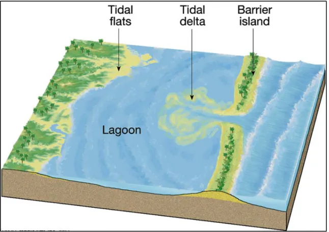
The depositional setting for the Tilje Formation varied through time, and consisted of tide-dominated deltaic, estuary, and embayment environments (Figure 5).

Figure 5. Sedimentary depositional environments. (Verlo and Hetland, 2008 )

The variation was caused by the syn-depositional tectonic movement, which allowed for both the increased accommodation space, and then as uplift occurred, a shift towards mixed- and fluvial-dominated environment (Martinius et al., 2005). The shift in depositional environment results in alterations to both facies distribution and stacking patterns. The formation can be subdivided into four facies zones based on variations in lithology, which can be correlated to changes in sea level (Figure 6). Identifying and interpreting this facies variation is crucial reservoir characterization (Martinius et al., 2005). The top two zones are tidally influenced deposits, while the lower two zones are

Figure 6. Norne Field stratigraphic units subdivided into facies types. (Statoil, 2001)

typically bay deposits or mouth bars (Statoil, 2001). Depositional environments such as these tend to be highly heterolithic at all scales, prone to a highly channelized shoreline ,and possess wide variations in grain size and distribution (Galloway, 1975). The Tilje

Formation consists of mudstone and fine-to-coarse grained, well-sorted sandstone. The presence of limestone stringers and carbonaceous layers can also be found within the Tilje Formation (Statoil, 2001). The Tilje Formation sediments were deposited from the West and major tectonic uplift led to erosion in the North, resulting in an unconformity at the top of the Tilje Formation (Statoil, 1995). The variations in depositional

environment results in a wide range of grain sizes and distribution (Figure 7), as well as increased volumes of shale and mud (Ichaso et al., 2009).

Petrophysical properties are also difficult to assess in heterolithic reservoirs, such as the Tilje Formation. In particular, porosity and permeability values can vary widely, both vertically and horizontally, within heterolithic reservoirs (Ringrose et al.,

2005). Net sand calculations can be greatly impacted by the thin, interbedded mud deposits within the heterolithic reservoir. Multiple studies (Flolo et al., 1998; Nordahl et al., 2005; Ringrose et al., 2005) state the best way to characterize the heterolithic

reservoir is by subdividing into facies using mineralogical, nuclear magnetic resonance logging, or photoelectric data to identify pore-scale characteristics and by identifying pressure trends. Additionally, diagenesis can impact reservoir quality in multiple ways. One way, which is prevalent in shaly sandstone reservoirs, is the effect of faulting. Faulting can cause a loss of porosity and permeability within the reservoir due to juxtaposition and clay smearing. Another form of diagenesis in the Tilje Formation, which occurs with increasing burial depth, is the growth of grain-coating clay minerals.

The presence of chlorite, chlorite/illite, and illite minerals can prevent the quartz precipitation, which would naturally occur with increasing temperature and pressure, decreasing porosity and permeability (Figure 8). In areas within the Tilje Formation, increased cementation caused by quartz precipitation, result in a decrease in permeability and porosity (Martinius et al., 2005). The structural and tectonic evolution of the Norne Field was both essential and adverse to the development of a high quality hydrocarbon reservoir. The sedimentology and stratigraphy of the complex, heterolithic Tilje Formation, however, is also a limiting factor in petroleum reservoir characterization. Therefore, it is as crucial to account for stratigraphic and structural variables within the Tilje Formation the Norne Field.

1.2.3 Previous Research on Rock Physics

Geoscientists have been using rock physics models to link petrophysical properties (lithology, porosity, permeability, etc.) to geophysical methods

(compressional velocity, shear velocity, acoustic impedances, etc.) for decades. Rock physics accounts for several variables, including: mineralogy, porosity, pore shape and size, pore fluid, pressure and temperature. Other factors that can impact a rock physics model are the presence of faults and fractures, which can significantly impact a

reservoir. With so many variables, the common practice has been to make assumptions for those parameters that are the most difficult to measure. Models such as the time-average equation (Wyllie et al., 1956) and others commonly used (Hertz, 1882; Mindlin, 1949; Gassman, 1951) are based on empirical observations between porosity and

pore structure is simplified by assuming the rock is composed of spherical grains; this does not account for the impact of irregularly shaped pores or clay minerals on the acoustic response of the rock. While these models can be applied to an ideal sandstone reservoir, they are severely lacking in providing accurate details within an argillaceous sandstone reservoir. Cross-plot techniques and characteristic patterns are utilized to build correlations between porosity and compressional velocity, however, previous methods (Raymer et al., 1980; Gardner et al., 2005) cannot account for scattering that

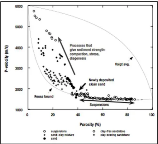
Figure 9. Results of multiple experimental studies indicate patterns of lithology in the compressional velocity-porosity relationship. (Mavko et al., 2003)

accompanies field measurements. Additional studies (Han et al., 1986; Tosaya et al., 1982; Kowalis et al., 1984) have identified the source of the scatter to be attributed to variations in clay content. These previous studies have been able to account for the scatter, however, the data used is not easily available, or the model requires too many input parameters to be readily applied. These studies provide a solid foundation for velocity-porosity relationship in shaly sandstone reservoirs, which are greatly affected by variations of clay content. Marion et al. (1992) observed that with increasing clay content compressional velocity (Vp) will increase until a critical value of clay was reached, which the authors gave a range of 20-40 percent, then compressional velocity decreases with increasing clay content. Unfortunately, when applied to field

measurements, this inverted V shape (Figure 10) rarely exists. The previous studies have

Figure 10. Inverted V-shape illustrating the effect of increasing amount of clay on porosity and compressional velocity. (Marion et al., 1992)

aided in shaping the known relationship between acoustic velocity and porosity, but most are not easily applied to field data and several do not account for the difference in pore structure between spherical quartz grains and elongated clay minerals. A new rock physics model was developed by Adesokan (2012), which modifies the Sun rock physics model to be applied specifically to shaly sandstone reservoirs, and uses measurements that are commonly available in petroleum exploration. This type of model and method will aid greatly in hydrocarbon exploration and production, within argillaceous

2. METHODS 2.1 Sun Rock Physics Model

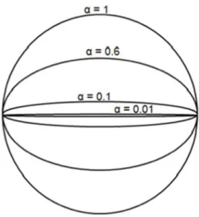
The Sun rock physics model (Sun, 2000; Sun, 2004) identifies the importance of pore structure difference between quartz grains and clay mineral components, and the effect these changes have on acoustic waves travelling through them. The model accounts for the difference between the spherical quartz grains and the elongated clay minerals, to predict a pore aspect ratio (Figure 11). This pore aspect ratio (PAR) can then be used to identify a critical volume of clay, which signifies the change from a sand load bearing to a clay load bearing rock. This threshold correlates with a drastic shift in the petrophysical and acoustic behavior of the reservoir. The theoretically derived Sun (2000) forward model provides a simplified mathematical link between elastic properties

and the pore structure of rocks by identifying frame flexibility factors (f, γ, Fk). These

frame flexibility factors are used to identify the impact of pore structure on acoustic velocity. By applying the forward model, a theoretical value can be generated and compared to measured values in order to confirm the validity of the model. Sun’s (2000) forward model is as follows:

For theoretical density:

For theoretical bulk and shear moduli:

√

The variables C and D in Equations (4) and (5) are for compressibility, which is the inverse of the bulk (K) and shear (μ) moduli. Next, the application of the Sun rock physics model to the well logs requires the inverse model:

(

)

When applying the Sun (2000) model it is beneficial to begin with the solving for the pore structure parameter (γ) related to the shear modulus. The reason for this is that the equation for shear modulus of a fluid (modified Equation 5) simplifies a portion of the equation to:

Therefore, solving for the shear modulus of the dry-rock frame is exactly equal to the shear modulus obtained from the well log data:

This estimation simplifies solving for the pore structure parameter (Equation 7) to:

Solving for the pore structure related to shear modulus is, therefore, quick and simple. It is important to note that the pore structure parameter for the shear and bulk moduli are not the same, and must be calculated individually. The simplified shear modulus

equations also provide the ability to quality control the calculations before progressing to the more complicated pore structure parameter related to the bulk modulus.

The pore structure parameter (γ) is a measure of the rock frame flexibility under deformation due to pore structure (Sun, 2000; Sun, 2004):

(12)

Other factors can influence the pore structure within a reservoir, however, and must be accounted for in order to obtain more accurate results. Factors directly impacting pore structure within the Tilje Formation in the Norne Field include: facies variation, diagenesis, and fracturing caused by faulting. (Maritinius et al., 2005) The onset of diagenesis in the Norwegian Sea begins at 2500-3000 meters. (Ramm et al., 1994) Within the area of interest for this study, the Tilje Formation ranges in depth from 2700 to 3500 meters, implicating that the pore structure may be impacted by diagenesis due to increased burial depth.

The Sun (2000; 2004) rock physics model allows for the variations in acoustic response due to pore structure changes. Variations in pore structure can be lithological (e.g. quartz grains and clay minerals) or can be caused by mechanical alterations. For instance, fracturing or cementation within a reservoir can impact the gamma (γ) parameter value. (Adesokan, 2012) Marion et al. (1992) and Yin (1993) developed methods for identifying critical clay volume using cross-plots and specific representative patterns, however, field measurements rarely follow the predictive patterns. Adesokan (2012) developed an alternative method of identifying the critical clay volume using materials that are readily available in most argillaceous sandstone reservoir evaluation. 2.2 Hertz-Mindlin and Sun Model

on compressional velocity using multiple ordinary differential equations. Adesokan (2012) used differential effective medium (DEM) equations to numerically predict the effect of pore aspect ratio on compressional velocity. The result of the DEM supports the use of the Sun rock physics model as a method for estimating pore structure from well logs. Sun’s rock physics model (Sun, 2000) was modified by Adesokan (2012) to predict velocity through a shaly sandstone reservoir, using an adaptation of the Hertz-Mindlin model for non-cemented formations. Hertz (1882) and Mindlin (1949) developed models for predicting velocity in non-cemented formations using:

[

]

[

]

The Hertz-Mindlin (HM) model identifies two end members of the elastic moduli-porosity relationship; (1) depositional moduli-porosity (~40%) and (2) zero moduli-porosity. The model is designed to predict porosity reduction caused by differential sorting (Adesokan, 2012). The ultimate result of the HM model is to predict the dry bulk (Kdry)and shear (μdry)

moduli by relating it to porosity. The modified Hertz-Mindlin and Sun (HMS) model accounts for the variation in pore structure. Adesokan (2012) improved the theoretical and measured velocity-porosity relationship accuracy of 65% (Figure 12) compared to the Hertz-Mindlin model previously used in velocity estimation. The HMS model

replaces Equations (4) and (5) in Sun’s model with Equations (6’) and (7’) below:

[

]

[

]

Resulting in a theoretical velocity calculation of:

_√

(8’) The HMS modification greatly improved the ability to predict the P-wave velocity

Figure 12. The measured vs theoretical results of the Hertz-Mindlin model (a) and the increased accuracy (by 65%) of the relationship using the Hertz-Mindlin and Sun model. (Adesokan, 2012)

through a shaly sandstone reservoir. Additionally, the model provides the link between the pore structure parameter and the PAR of the reservoir, using Equation (15).

minerals, with an upper and lower boundaries of 1 (pure clay) and 0.5 (pure quartz). (Adesokan, 2012) The HMS model offers three fundamental results: (1) quantitative description of pore structure; (2) critical clay volume; and (3) increased understanding of the correlation between porosity and velocity. Traditionally, acoustic impedance and porosity have been correlated at the well log scale, which allows geoscientists to predict porosity from post-stack seismic data using inverse theory. However, the ability to use inversion methods to predict PAR from post-stack seismic data would greatly enhance reservoir characterization methods.

2.3 Relations between Acoustic Impedance and Reservoir Properties

Geophysicists and petrophysicists use the strong linear correlation between acoustic impedance and porosity to interpret seismic inversion results. The formula typically used is:

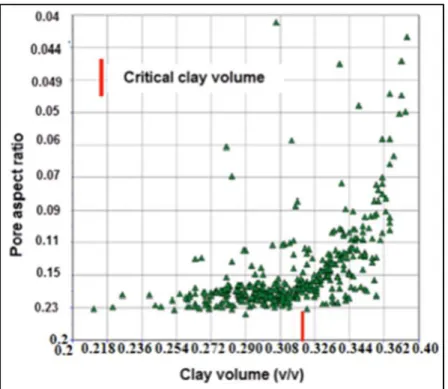
Figure 13. Results of Adesokan (2012) illustrating the critical clay volume relationship with the pore aspect ratio, utilizing the HMS rock physics model.

Zhang et al. (2012), using the modified Sun model, identified the relationship between the acoustic impedance and the product of the frame flexibility factor (γ) and porosity dramatically improved the acoustic impedance-porosity correlation. The equation is as follows:

Where, A and B are field specific values, γ is the pore structure parameter and φ is porosity. Figure 14 illustrates the improved relationship between acoustic impedance and

the product of the pore structure parameter and porosity. The improved correlation between acoustic impedance and the product of the frame flexibility factor and porosity indicates that seismic inversion results for acoustic impedance can be directly linked to pore aspect ratio. Since pore aspect ratio has been used for many years to determine the shaliness of a sandstone reservoir, the improved relationship between porosity and

velocity, provided by Adesokan (2012) and Zhang et al. (2012), will be incredibly beneficial in identifying the PAR distribution within a clastic reservoir from seismic data.

2.4 Seismic Analysis and Inversion

Seismic inversion is the process of converting geophysical measurements (Vp/Vs, AVO, acoustic impedance, etc.) to reservoir properties (lithology, porosity, etc.). This process is crucial to the exploration and production of hydrocarbons as it allows geoscientists to provide reservoir properties, identified at the borehole, to an entire field. There are multiple types of inversion: linear, non-linear, deterministic, stochastic, elastic, etc. It is important to understand each type of inversion to know which is necessary for a given situation. The objective for this study is the spatial distribution of clay content, and the available seismic volume is post-stack time-migrated (PSTM). The best method for this situation, according to Table 1, is a deterministic inversion for acoustic impedance. The

convolutional model used in this study is based on well log data, which provided the synthetic seismic data required for the inversion process. Model-based, deterministic inversion requires three main inputs to successfully generate an acoustic impedance volume. First, is the seismic volume; two- or three-dimensional volumes can be utilized depending on the scope of the study, the availability of data, and computing power. Second, a wavelet is generated from the model to establish the link between seismic and borehole scales. Lastly, a low frequency model is needed to constrain the inversion and to provide information from well log data. In order to build the low frequency model, it is necessary to conduct seismic horizon and fault interpretation, as well as conduct seismic-well-ties (Bui et al., 2012). Seismic inversion is not a simple process. Establishing the link between seismic and well log data is an iterative procedure that requires detailed effort with extensive quality control. Figure 16 illustrates an example seismic inversion workflow for post-stack inversion.

3. INTERPRETATIONS 3.1 Application of HMS Model to Norne Field

Applying the HMS model to the Norne Field should, theoretically, result in a similar response to that of Adesokan (2012). Interpreting the results of the pore structure parameter proved to be more complex than the example provided by Adesokan (2012) for several reasons. First, Adesokan (2012) applied the HMS model to a 60-meter thick interval, while the interval used in this study ranged from 100 to 200 meters in thickness. This increase in volume corresponds to large variations in depositional environment of the Tilje Formation, meaning that the pore structure will have a wider range of variables throughout the interval. Second, the depth of burial used in the Adesokan’s (2012) analysis was at depths ranging from 1630-1693 meters, avoiding the impact of

diagenesis. The average depths in this study were from 2700-3000 meters, with the onset

Figure 16. Adesokan (2012) results of (a) HMS model and (b) the results of this study.

of diagenesis occurring at an estimated 2500-meter depth. (Ramm et al., 1994) Finally, fracturing decreases the pore aspect ratio and can complicate the analysis. Identifying and understanding how these additional variables impact the acoustic impedance-pore structure parameter relationship is crucial to successfully applying the HMS rock physics model. This interpretation is based on identifying the limestone stringers, literature review detailing possible cementation and diagenesis, and well log analysis. Heslop and Heslop (2003) published methods of analyzing shaly sandstones based on well log response. The methods identify trends based on gamma ray, density, and neutron porosity relationships. Figures 18-20 illustrate the theoretical trend and the trends found in this dataset.

Figure 18. Interpreting shaly sands using gamma ray and bulk density. (Heslop and Heslop, 2003)

Figure 19. Interpretation of the Tilje Formation using gamma ray and bulk density.

Shaly Sandstone, clay replaces fluids in intergranular pore space Cemented Sandstone/ Limestone Stringers

Figure 20. Interpreting shaly sands using gamma ray and neutron porosity. (Heslop and Heslop, 2003)

Figure 21. Interpretation of shaly sands using gamma ray and neutron porosity. Shaly Sandstone,

clay replaces fluids in intergranular pore space Cemented Sandstone/ Limestone Stringers

Based on the interpretation methods established by Heslop and Heslop (2003), the mismatch between Adesokan’s (2012) results and the results of this study are directly related to the impact of diagenesis, cementation, clay replacing fluid in pore space, and the assumption that only sand and shale exist in the system. Further understanding of the relationship between pore structure and the elastic properties of the Tilje Formation is needed to complete the analysis.

3.2 Bulk Density

Theoretical bulk density can be used to calibrate the solid matrix that will be used for the remaining calculations in this study. Using Equation (1) to calculate

theoretical bulk density will insure that the proper solid matrix will be chosen throughout the rock physics process. Based on information provided in the dataset, the Tilje

Formation is almost completely water saturated throughout the Norne Field. The Kf in Equation (4) can be replaced with the bulk modulus for brine, which is 2.3281 GPa. Also, because the dataset did not contain any core analysis or photoelectric logs, the density, shear and bulk moduli of the rock-forming minerals (ρs, μs and Ks) were estimated within the Tilje Formation. Additional inputs for the rock physics model can be found in Table 2.

A general description of the entire formation indicated the presence of limestone stringers throughout the formation, however, there is no provided method of

quantification and their vertical and spatial distribution are both limited. (Statoil, 2000) One method of potentially quantifying the limestone stringers is to run a multi-mineral analysis using available well logs, but without PE or imaging logs the necessary inputs

Table 2. Inputs into HMS rock phyics model. (Statoil, 2001)

must come from sonic response. Since the rock physics model used in this study also depends on inputs from the sonic logs, this type of multi-mineral analysis would provide skewed results. An assumption of the mineralogy, therefore, is necessary for this study. Using the assumption that everything that is not shale is sand, and generating a

theoretical bulk density allows the ability to identify the limestone stringers and explain their impact on the rock physics analysis (Figure 22). Based on the results of the

theoretical bulk density and being able to identify the limestone stringers, the assumption used in this study should satisfy the required inputs for the HMS model.

Figure 22. Theoretical bulk density versus measured bulk density. The limestone stringers are highlighted in maroon, with their locations displayed in the log track.

3.3 Shear Modulus

The relationship between shear modulus and porosity has been experimentally shown to display a predictable trend with increasing clay content (Han et al., 1986). Calculating the Voight and Reuss bounds was necessary to generate the Voight-Reuss average, which was used to generate both μs and Ks (Voight, 1928; Reuss, 1929). The increasing volumes of clay, which correspond to decreasing porosity values, cause an increase in the shear modulus. Additionally, clay infill occurs when clay minerals fill the pore space left by quartz grains, instead of fluids. This clay infill impacts the shear modulus by initially increasing the shear modulus, and then when a critical amount is achieved (~20-40%) the shear modulus is greatly reduced. (Adesokan, 2012) Figure 23

Figure 23. Predicted shear modulus response with varying amounts of clay infill. (Adesokan, 2012)

Figure 25. µ/µs as a function of porosity for the Tilje Formation.

illustrates this effect with increasing clay infill. The shear modulus-porosity relationship for the Tilje Formation is illustrated in Figure 24. The wide range of values at a fixed porosity (15%) is indicative of a clay infill corresponding to Figure 23(b) and (c), with clay infill ranging from 30-70 percent. This shear modulus-porosity relationship can be seen clearly upon solving for the pore structure parameter related to the shear modulus. Figure 25 illustrates the shear modulus-porosity relationship, color-coded with the pore structure parameter. The vertical axis in Figure 25 represents the normalized shear modulus, µ/µs. The increasing pore structure parameter corresponds with an increase in scattering of the shear modulus. Thus, the response of the Tilje Formation is similar to

that seen in experimental settings. A similar relationship can be seen with the bulk modulus-porosity relationship.

3.4 Bulk Modulus

The available dataset did not contain any mineralogical data in order to

quantitatively account for the varying lithological components, therefore, an assumption was required. The bulk modulus of the rock-forming minerals (Ks) was calculated using the volume of shale, determined using the gamma ray log, and assuming everything not shale to be sand. The assumption that only sand and shale exist in the Tilje Formation will underestimate the Ks value and cause impossible results in the petrophysical and rock physics calculations. These results, which were directly related to the presence of limestone stringers, were removed from the rock physics calculation to avoid distortion. The bulk modulus-porosity relationship agrees with Adesokan’s (2012) predicted

relationship, where the increase in clay infill values cause scattering and an initial increase in bulk modulus values. This is why a low pore structure parameter (high PAR) produces an increased Kb value, which is counterintuitive. The majority of the results, however, behave similarly to experimental trends, thus the model remains valid. Now that the model has been verified, the compressional and shear velocity-porosity

relationships can be analyzed to predict clay content and potentially link to seismic data. 3.5 Compressional and Shear Velocity

Compressional (P-wave) and shear (S-wave) velocities travel through rock in experimentally proven ways and, thus, are used extensively in the exploration of hydrocarbons. P-waves and S-waves generate different seismic attribute responses and

can be utilized to identify gas- and fluid-bearing zones, as well as structural and stratigraphic traps (Caldwell et al., 1997). Compressional and shear velocity-porosity relationships have also been used to predict the critical clay content, and in some cases are quite effective (Marion et al., 1992). However, as can be seen in Figure 28, there is no discernable shape to easily discern this boundary. The application of HMS model has been able to identify that critical clay volume with much higher accuracy. By adding in the calculated pore structure parameter, scatter still exists, but the reasoning of the dispersion becomes evident. The general trend, as expected is the decrease in velocity with increasing porosity. There are some areas that display increases in velocity, but

maintain a high PAR (sand). This is counterintuitive, but can be explained by

compaction and cementation effects on the sandstone facies. The same relationship can be seen in the shear velocity-porosity relationship (Figure 29), however the effects of fluid cause additional scattering in shear velocity.

Another method of attempting to distinguish the shale sand boundary is by cross plotting Vp/Vs versus depth. (Castagna et al., 1985) Figures 30 and 31 illustrate the predicted trend and the results from this dataset. The Vp/Vs – depth relationship in Figure 30 displays a kink in the sandstone curve. Castagna et al. (1985) used

Gassmann’s equations to calculate theoretical compressional velocity in water-saturated sandstones. Gassmann’s equations predict an exponential increase in velocity due to

Figure 30. Theoretical model of shale and sandstone for Vp/Vs ratio vs depth. (Castagna et al., 1985)

increasing water saturation, until reaching one hundred percent saturation, and then the increase is linear with depth (Castagna et al., 1985). The sandstone line decreases with increasing depth in an exponential manner, similar to that of the shale line, however, once the sandstone becomes one hundred percent water saturated, the line transitions to a straight line. The Vp/Vs –depth relationship readily identifies the two main zones, and four total zones, of the Tilje Formation. This transition corresponds with a decrease in sea level, and a transition from a deeper shale-dominated lithology to moderately cleaner sands. Understanding the impact that clay content can have on velocities is crucial when relating petrophysics to seismic responses. Previously, Vp/Vs ratios have been utilized to identify net sand zones in a reservoir, but the relationship can be greatly impacted by the presence of fluids, gas, and clay volume. (Castagna et al., 1985) These relationships,

Figure 31. Interpreted zones within the Tilje Formation using Vp/Vs ratio and depth.

therefore, are not sufficient for the purposes of this study, so a different variable is needed.

3.6 Acoustic Impedance-Porosity Relationship

Acoustic impedance is the product of density and acoustic velocity. Density variations can impact acoustic impedance, especially in this study due to the

mineralogical assumption, but changes in velocity have a greater effect. A change in porosity (Figure 32), from 0-35% for example, would cause a decrease in velocity by up to 1500 m/s. (Dolberg et al., 2000) The greatest impact to the velocity variation is the material the seismic waves travel through. For example, a softer rock, or one that

Figure 32. Velocity variations with increasing porosity. (Dolberg et al., 2000)

contains fluid, will result in a decrease in velocity. Based on this established

relationship, acoustic impedance can thereby be used to estimate reservoir properties, such as porosity. Figure 33 displays the acoustic impedance-porosity relationship with a linear trend showing a R2 _{= 0.61 correlation. The acoustic impedance-porosity}

relationship is the basis for most rock physics and geophysical methods of interpretation and is crucial in linking well log and seismic data, through inversion methods. This relationship is typically linear, which allows the conversion from acoustic impedance to porosity to be a simple equation. This relationship is typically sufficient, but Zhang et al. (2012) have developed a new variable that improves upon this relationship.

Figure 33. Acoustic impedance vs porosity for the Tilje Formation.

3.7 Acoustic Impedance-Product (γ*Φ) Relationship

The improved relationship established by Zhang et al. (2012) involves the

product of the pore structure parameter and porosity, using Equation (18). In Zhang et al. (2012), the relationship between the product (gamma and porosity) and acoustic

impedance in carbonates was greatly improved. Applying this method to a shaly

sandstone reservoir produced results that were similar, but not as drastic. Figures 34 and 35 illustrate the improved relationship of AI-porosity and AI-product. The AI-product has a stronger correlation, but it is necessary to move from a simple linear equation to a polynomial equation in order to see the improvement. The results from the polynomial

regression for the AI-porosity relationship showed no improvement. The AI-product relationship, however, had an increased correlation by almost ten percent. The AI-product relationship is, therefore, a better option for this study than the traditional method. The following equation was modified from Equation (15) and is necessary to transition from the well logs to the post stack seismic data:

Figure 34. Acoustic impedance vs porosity, color-coded with the pore structure parameter, for the Tilje Formation.

AI = 9730-11840*ϕ R2=0.61

Figure 35. Acoustic impedance vs. the product of the pore structure parameter and porosity.

3.8 Seismic Analysis and Inversion Interpretation

Seismic well ties, horizon interpretation, and structural analysis were performed on the post-stack seismic dataset. This provided the framework for the low frequency model, which is necessary to provide a link between well log data and seismic data. The three dimensional seismic volume provided in the dataset ranges from approximately 8 Hz to 65 Hz, based on spectral decomposition. The low frequency model bridges the gap between 0 and 8 Hz, allowing the connection between scales. Deterministic seismic inversion was used because it results in one, best-case scenario for the provided dataset. In the petroleum industry, post-stack seismic data is the most commonly utilized data type. The seismic variables that inversion produces are somewhat limited in post-stack seismic data, thus making the HMS rock physics model appealing in this situation.

AI = 1590(ϕγ)2-4380(ϕγ)+9940

Figure 36. Seismic interpretation of the Norne Field, indicating well locations.

The inversion parameter being utilized in the post-stack seismic data was acoustic impedance.

The results of the inversion displayed a range of acoustic impedances throughout the Tilje Formation. In particular, one area within the main section displays very high acoustic impedances (8-9 MRayls), which based on the HMS model correspond to shale zones. Figures 37 and 38 depict the inline and crossline closest to the predicted shale zone.

Figure 37. Inversion results on Inline 1083 in the Norne Field, with the circle denoting the high AI anomaly.

Figure 38. Inversion results for Xline 1103 in the Norne Field, with the circle denoting the high AI anomaly

.

Figure 39. Inversion results averaging the response within the Tiljge Formation. The circle denotes the high AI anomaly and the lines denote the location of inline and xline displayed in previous images.

In order to confirm the results of the inversion, a qualitative well log analysis was conducted based on gamma ray logs and the well location in relation to the shale zone. The well logs located nearest the shale zone have a higher volume of shale than those located in areas outside the high acoustic impedance zone determined with the inversion. Figure 40 displays the average acoustic impedance through the entire 100-200 meter Tilje Formation. A better understanding of the vertical and spatial distribution of

acoustic impedance can be seen in time slices taken throughout the interval (Figure 41).

Figure 40. Location of key wells around AI anomaly, with gamma ray logs depicting increasing shaliness near anomaly.

The complex geometry of the Norne Field caused the time slices to display data within the Tofte Formation (above the Tilje Formation) and the Aare Formation (below the Tilje Formation) in some areas of the field.

While the spatial distribution of acoustic impedance is important, reservoir properties are more important to hydrocarbon exploration and production. The acoustic impedance volume was, therefore, converted to both porosity and the product (γΦ) volumes, using the following equations from the rock physics analysis:

And,

The spatial distribution of porosity (Figure 42) changes both horizontally and vertically within the Tilje Formation. In the southwest area of the Norne Field, porosity decreases with depth, from approximately 30-5 percent. Utilizing the same method, but computing a volume displaying the product (γΦ), the variation of clay content can be visualized (Figure 43). Shale has pore aspect ratio of approximately 0.04-0.1, or a pore structure parameter of 10-25, and porosity values that range from 5-15 percent. The product (γΦ), therefore, will range from 0.04-1.5, with the higher values relating to clean sands and lower values relating to shale zones. In Figure 43, in the 2525 ms map, the highest product values are in the southwest zone of the Norne Field. According to qualitative well log analysis this zone corresponds to clean sands with high porosity. As depth increases within the Tilje Formation, the value of the product drops to 0.04, which corresponds to shale zones. The time slice maps corresponding to the product, therefore,

provide enhanced reservoir characterization of the Tilje Formation. While the porosity and product images appear similar, there are some areas of distinct differences that illustrate that porosity and lithology are not synonymous. Since porosity values typically decrease with depth, having only porosity does not provide enough information in regards to changing lithology. The product (γΦ), however, provides a direct link to lithology for improved reservoir characterization. Additionally, using the acoustic

Figure 41. Acoustic impedance time slices through the Tilje Formation. N N

N

impedance-product relationship provided an increase in resolution, which can be seen by comparing Figures 42 and 43. This enhanced resolution can be crucial in the decision-making process for field development.

In order to quality control the results of generated porosity and product volumes, the time slices shown in Figures 42 and 43 were compared between two wells in

different parts of the field. Well C-3H (Figure 44) is located at the southwest part of the

Figure 42. Porosity time slices through the Tilje Formation. N N N

field, in an area that appears to be dominated by higher quality sands. Well C-4AH (Figure 45) is located near the center of the field, in an area that seems dominated by shale. The results indicate that the seismic time slices do, in fact, agree with the well log data. Specifically, the porosity decreasing with depth and the increase in gamma ray as increased amounts of shale are evident. The density spikes that appear to be occurring are due to the presence of limestone stringers. Both well logs clearly depict porosity and

Figure 43. Product time slices through the Tilje Formation.

N N N

lithology are not synonymous and each need to be addressed separately. In fact, while the average for the entire interval displays Well C-4AH as being dominated by shale, there are clearly zones of good sand found within the well, which can potentially aid in reservoir connectivity.

4. CONCLUSIONS

The structural complexity of the Norne Field has long been thought to be the cause of reservoir discontinuity. In particular, most geoscientists have postulated that this discontinuity is due to faults that remain below seismic resolution. Another reason for reservoir discontinuities are zones of clay content that were formed by deposition or possible reworking during structural evolution. Applying and analyzing the HMS rock physics model to the Norne Field provided enhanced reservoir characterization of the Tilje Formation. The HMS model was successfully applied to an incomplete dataset, with the only major assumption being the mineralogical composition of the reservoir. It is also crucial to identify the impact of depth (temperature and pressure) on the

mineralogical composition within the reservoir. Heterolithic reservoirs, such as the Tilje Formation, can be very complicated due to both deposition and diagenetic processes. Core data, or mineralogical data based on core, would be beneficial to improve the results of the HMS model.

Post-stack seismic inversion is a useful tool to analyze the variability in rock type within a reservoir, depending on resolution. The seismic inversion results of this study depicted a high acoustic impedance anomaly within the Tilje Formation, which the HMS model predicts to be a shale zone. The qualitative well log analysis of well located near the anomaly is in agreement with results of the HMS model. The maps generated by converting acoustic impedance to porosity and the product (γΦ) provide enhanced reservoir characterization. The product time slices display isolated zones of shale that can cause baffles to flow and decrease production. Additionally, the AI-(γΦ) relationship

provided enhanced resolution compared to the traditional AI-Φ method. Images that are generated by this method can be a great aid in field development and production.

Provided that understanding of the geologic process and the availability of mineralogical data, the HMS model would be an extremely useful tool for the exploration and

production of argillaceous sandstone reservoirs. The ability to apply the HMS model to a basic dataset can be an asset when time and computer power are limited. With further successful application and modification, the model and method could potentially be applied to both conventional and unconventional reservoirs to aid in reservoir

characterization and maximizing hydrocarbon production within argillaceous sandstone reservoirs.

REFERENCES

Adesokan, H. 2012, Rock Physics Based Determination of Reservoir Microstructure for Reservoir Characterization. Doctoral Thesis Dissertation. Texas A&M

University, College Station, Texas.

Ammah, A.N., 2012, Applying time-lapse seismic inversion in reservoir management: A case study of the Norne Field. Masters Thesis. Department of Petroleum E

ngineering and Applied Geophysics, Norwegian University of Science and Technology, Trondheim, Norway.

Blystad, P., Brekke, H., Faerseth, R.B., Larsen, B.T., Skogseid, J., Torudbakken, B., 1995, Structural elements of the Norwegian continental shelf. Part II The

Norwegian Sea Region: Norwegian Petroleum Directorate Bulletin, vol. 8, 45 pp. Brekke, H., Dahlgren, S., Nyland, B., Magnus, C., 1999, The prospectivity of the Voring

and More basins on the Norwegian Sea continental margin: Petroleum Geology of Northwest Europe: Proceedings of the 5th _{Conference, 261-274.}

Caldwell, J., Chowdhury, A., Van Bemmel, P., Engelmark, F., Sonneland, L., Neidell, N. S., 1997, Exploring for Stratigraphic Traps: Oilfield Review, pp. 48-61. Castagna, J.P., Batzle, M.L., Eastwood, R.L., 1985, Relationships between

compressional-wave and shear-wave velocities in clastic silicate rocks: Geophysics, vol. 50, pp. 571-581.

Cooke, D., Cant, J., 2010, Model-based seismic inversion: comparing deterministic and probabilistic approaches: CSEG Recorder, pp. 28-39.

2000, Porosity prediction from seismic inversion, Lavrans Field, Halten Terrace, Norway: The Leading Edge, pp. 392-399.

Faerseth, R.B., 2012, Structural development of the continental shelf offshore Lofoten- Vesteralen, northern Norway: Norwegian Journal of Geology, vol. 92., pp 19-40. Flolo, L.H., Menard, W.P., Weissenburger, K.W., Kjaerefjord, J.M., Amesen, D.M.,

1998, Revealing the petrophysical properties of a thin-bedded rock in a

Norwegian Sea reservoir by the use of logs, core, and miniperm data: Society of Petroleum Engineers, vol. 49326, pp. 815-830.

Galloway, W.E., 1975, Process framework for describing the morphologic and stratigraphic evolution of deltaic depositional systems, In: Deltas: Models for Exploration (Ed. M.L. Broussard), pp. 99-149. Houston Geol. Soc.

Gassmann, F., 1951, Elasticity of porous media: Vierteljahrsschrder Naturforschenden Gesselschaft, vol. 96, 1-23.

Han, D.-h., A. Nur, and D. Morgan, 1986, Effects of porosity and clay content on wave velocities in sandstones: Geophysics, vol. 51, 2093-2107.

Hertz, H., 1882, On the contact of rigid elastic solids and on hardness, paper 6: Macmillan.

Heslop K, Heslop A. Interpretation of shaly-sands. Archive Template, (2003-04- 08)[2013-03-19]. http://www.lps.org.uk/docs/heslop_shaly_sands. pdf, London Geophysical Society, 2003.

Ichaso, A.A., Dalrymple, R.W., 2009, Tide-and wave-generated fluid mud deposits in the Tilje Formation (Jurassic), offshore Norway: Geology, vol. 37, pp. 539-542.

Klimentos, T., 1991, The effects of porosity-permeability-clay content on the velocity of compressional waves: Geophysics, vol. 56,1930-1939.

Kowallis, B. J., L. E. A. Jones, and H. F. Wang, 1984, Velocity-porosity-clay content systematics of poorly consolidated sandstones: Journal of Geophysical Research., vol. 89,pp. 10355-10364.

Langrock, U., Stein, R., 2004, Origin of marine petroleum source rocks from the Late Jurassic to Early Cretaceous Norwegian Greenland Seaway-evidence for

stagnation and upwelling: Marine and Petroleum Geology, vol. 21, pp. 157-176. Marion, D., A. Nur, H. Yin, and D. Han, 1992, Compressional velocity and porosity in

sand-clay mixtures: Geophysics, vol. 57, pp. 554-563.

Martinius, A.W., Ringrose, P.S., Brostrom, C., Elfenbein, A., Naess, A., Ringas, J.E., 2005, Reservoir challenges of heterolithic tidal sandstone reservoirs in the Halten Terrace, mid-Norway: Petroleum Geoscience, vol. 11, pp. 3-16.

Mavko, G., Mukerji, T., Dvorkin, J.,2003, Rock Physics Handbook-Tools for Seismic Analysis in Porous Media. Cambridge University Press, Cambridge, UK. Mindlin, R. D., 1949, Compliance of elastic bodies in contact: Journal of Applied

Mechanics, vol. 16,259–268.

Nordahl, K., Ringrose, P.S., Wen, R., 2005, Petrophysical characterization of a heterolithic tidal reservoir interval using a process-based modeling tool: Petroleum Geoscience, vol. 11, pp. 17-28.

Ramm, M., Bjorlykke, K., 1994, Porosity/depth trends in reservoir sandstones: assessing the quantitative effects of varying pore-pressure, temperature history and

mineralogy, Norwegian shelf data: Clay Minerals, vol. 29, pp. 475-490. Raymer, L. L., J. S. Gardner, and E. R. Hunt, 1980, An improved sonic transit time-to-

porosity transform, Society of Petrophysicists & Well Log Analysts.

Reuss, A., 1929, Berechung der Fliessgrenze vonMischkristallen, Z. Angew: Math. Mech, vol. 9,55.

Ringrose, P., Nordahl, K., Wen, R., 2005, Vertical permeability estimation in

heterolithic tidal deltaic sandstones: Petroleum Geoscience, vol. 11, pp. 29-36. Statoil, 1994, Plan for Development and Operation, Reservoir Geology, Support

Documentation.

Statoil, 1995. Reservoir Geological Update After 6608/10‐4.

Sun, Y. F., 2000, Core-log-seismic integration in hemipelagic marine sediments on the eastern flank of the Juan De Fuca Ridge: ODP Scientific Results, vol. 168, 21-35.


Sun, Y.-F., 2004, Seismic signatures of rock pore structure: Applied Geophysics, vol. 1, 42-49.

Sun, Y. F., 2004, Pore structure effects on elastic wave propagation in rocks: AVO modeling: J. Geophys. Eng., vol. 1,268-276.

Thomas, E. C., and S. J. Stieber, 1975, The distribution of shale in sandstones and its effect upon porosity, Society of Petrophysicists & Well Log Analysts.

Tosaya, C., and A. Nur, 1982, Effects of diagenesis and clays on compressional v elocities in rocks: Geophys. Res. Lett., vol. 9, 5-8.

and 4D data from the Norne Field as a benchmark case for future reservoir simulation model testing: Masters Thesis, NTNU, Trondheim, Norway.

Vernik, L., 1998, Acoustic Velocity And Porosity Systematics In Siliciclastics: The Log Analyst, vol. 39.

Voigt, W., 1928, Lehrbuch der Kristallphysik, Teubner: Leipzig, 962.

Wyllie, M. R. J., A. R. Gregory, and L. W. Gardner, 1956, Elastic wave velocities in heterogeneous and porous media: Geophysics, vol. 21, 41-70.


Xu, S., and R. E. White, 1995, A new velocity model for clay-sand mixtures: Geophysical Prospecting, vol. 43, 91-118.

Yin, H., 1993, Acoustic velocity and attenuation of rocks: Isotropy, intrinsic anisotropy, and stress induced anisotropy: PhD, Stanford University.

Zhang, T., Dou, Q., Sun, Y., 2012, Improving porosity-velocity relations using carbonate pore types: Presented at 82nd _{Annual International Meeting, SEG.}