A Heuristic Search Algorithm for Flow-Shop Scheduling

A Heuristic Search Algorithm for Flow-Shop Scheduling

Joshua Poh-Onn Fan Graduate School of Business

University of Wollongong, NSW, Australia E-mail: [email protected]

Graham K. Winley

Faculty of Science and Technology Assumption University, Bangkok, Thailand E-mail: [email protected]

Keywords: Admissible heuristic function, dominance, flow-shop scheduling, optimal heuristic search algorithm Received: October 25, 2007

This article describes the development of a new intelligent heuristic search algorithm (IHSA*) which guarantees an optimal solution for flow-shop problems with an arbitrary number of jobs and machines provided the job sequence is constrained to be the same on each machine. The development is described in terms of 3 modifications made to the initial version of IHSA*. The first modification concerns the choice of an admissible heuristic function. The second concerns the calculation of heuristic estimates as the search for an optimal solution progresses, and the third determines multiple optimal solutions when they exist. The first 2 modifications improve performance characteristics of the algorithm and experimental evidence of these improvements is presented as well as instructive examples which illustrate the use of initial and final versions of IHSA*.

Povzetek: Opisan je nov hevristični iskalni algoritem IHSA*.

1

Introduction

The optimal solution to the flow-shop scheduling problem involving n jobs and m machines determines the sequence of jobs on each machine in order to complete all the jobs on all the machines in the minimum total time (i.e. with minimum makespan) where each job is processed on machines 1, 2, 3, …, m, in that order. The number of possible schedules is (n!)m and the general problem is NP-hard. For this general problem it is known that there is an optimal solution where the sequence of jobs is the same on the first two machines and the sequence of jobs is the same on the last two machines [4]. Consequently, for the general problem with 2 or 3 machines there is an optimal solution where the jobs are processed in the same sequence on each machine and the optimal sequence is among only n! job sequences. However, in the optimal solution for the general problem with more than 3 machines the jobs are not necessarily processed in the same sequence on each machine. This article is concerned with the development of an algorithm (IHSA*) which is guaranteed to find an optimal solution for flow-shop scheduling problems involving an arbitrary number of jobs and machines where the problem is constrained so that the same job sequence is used on each machine.

Early research on flow-shop problems is based mainly on Johnson’s theorem, which gives a procedure for finding an optimal solution with 2 machines, or 3 machines with certain characteristics [20], [21]. Other

hybrid approaches which combine different components of more than one metaheuristic [1].

An initial version of a new intelligent heuristic search algorithm (IHSA*) for flow-shop problems with an arbitrary number of jobs and machines and subject to the constraint that the same job sequence is used on each machine has been proposed in [6], [7], [8]. It is based on the Search and Learning A* algorithm presented in [44], [45], [46] which is a modified version of the Learning Real Time A* algorithm in [24], [25] which is, in turn, a modified version of the original A* algorithm [10], [12]. At the start of the search using IHSA* different methods are considered for computing estimates for the total time needed to complete all of the jobs on all of the machines assuming in turn that each of the jobs is placed first in the job sequence. It is shown that if there are m machines then there are m different methods that should be considered. Among the estimates associated with each method the smallest estimate is referred to as the value of the heuristic function that is associated with that method and it identifies the job that would be placed first in the job sequence at the start of the search if that method is used. If the value of the heuristic function does not exceed the minimum makespan for the problem then the heuristic function is said to be admissible and in such cases IHSA* is guaranteed to find an optimal solution provided the job sequence is the same on each machine. The proof of this result for IHSA* is given in [8] and is similar to that given in [22] and [23] in relation to the A* algorithm from which IHSA* is derived. The term “heuristic” is used in the title of IHSA* because the optimality of the algorithm and its performance depends on the selection of an appropriate admissible heuristic function at the start of the search and this function continues to guide the search to an optimal solution.

The purpose of this article is to describe the development of IHSA* which has occurred since the initial version was first presented in [6]. For simplicity of presentation the development is described in terms of problems involving an arbitrary number of jobs with 3 machines. However, the notations, definitions, proofs, and concepts presented may be extended to problems involving more than 3 machines if the job sequence is the same on each machine and these extensions are noted at the appropriate places throughout the presentation. Three significant modifications have been made to the initial version of IHSA*. The first concerns the choice of an admissible heuristic function at the start of the search. The second concerns the calculation of heuristic estimates as the search progresses, and the third determines multiple optimal solutions when they exist.

Following an introduction to the initial version of IHSA* each of the 3 modifications is presented. Experimental evidence of improvements in performance characteristics of the algorithm which result from the first 2 modifications is provided in the Appendix and discussed in section 5. Instructive examples are given to illustrate the initial and final versions of IHSA* and these have been limited to 3 machines in order to allow interested readers to familiarize themselves with the algorithm by reworking the examples by hand. The

proofs of results related to the modifications are presented in the Appendix.

2

The initial version of IHSA

*

Before presenting the initial version of the algorithm notations and definitions are introduced and the state transition process associated with IHSA* is described together with the features of search path diagrams which are used to illustrate the development of an optimal job sequence.

2.1

Notations and definitions

The following notations and definitions are introduced for a flow-shop problem involving n jobs J1, J2, …, Jn and 3 machines M1, M2, M3.

Oij is the operation performed on job Ji by machine Mj and there are 3n operations. For job Ji the processing times ai, bi, and ci denote the times required to perform the operations Oi1, Oi2, and Oi3, respectively and these processing times are assumed to be non negative integers. If Oij has commenced but has not been completed then pij represents the additional time required to complete Oij and at the time when Oij starts pij is one of the values among ai, bi, or ci. The sequence φst = {Js, …, Jt} represents a sequence of the n jobs with Js scheduled first and Jt scheduled last. T(φst) is the makespan for the job sequence φst and S(φst) is the time at which all of the jobs in φst are completed on machine M2.

Using these notations and definitions Figure 1 illustrates the manner in which the operations associated with the job sequence φst are performed on the 3 machines.

) ( st

Sφ

) (st

Tφ i

n

i a

∑

=

≥

1

i n

i b

∑

=

≥

1

i n

i c

∑

=

≥

1

Figure 1: Processing the Job Sequence φst

A method for calculating an estimate of the total time to complete all of the n jobs on all of the 3 machines when job Ji is the first job in the sequence is given by ai + bi + _i

n

i

c

∑

=1

. Then the heuristic function associated with this method is H3 where,

H3 = min [a1 + b1, a2 + b2, …, as + bs, …, an + bn] + i

n

i

c

∑

=1

. (1) If min [a1 + b1, a2 + b2, …, as + bs, …, an + bn] = as + bs then H3 = as + bs + _i

n

i

c

∑

=1

scheduled first in the job sequence. It is seen from Figure 1 and proved in the Appendix that H3 is an admissible heuristic function and H3 is the heuristic function that was used in the initial version of the IHSA*.

2.2

The state transition process

The procedure for developing the optimal job sequence using IHSA* proceeds by selecting an operation which may be performed next on an available machine. At the time that selection is made each of the 3n operations is in only one of 3 states: the not scheduled state; the in-progress state; or the finished state and the operation which is selected is among those in the not scheduled state. Operations not in the finished state are referred to as incomplete. A state transition occurs when one or more of the operations move from the in-progress state to the finished state and at any time the state level is the number of operations in the finished state.

IHSA* describes the procedure which takes the state transition process from one state level to the next and the development of the optimal job sequence is illustrated graphically using search path diagrams.

2.3

Search path diagrams

A search path diagram consists of nodes drawn at each state level with one of the nodes connected to nodes at the next state level. Each node contains 3 cells which are used to display information about operations on the machines M1, M2, and M3, respectively. When a state transition occurs one of the nodes at the current state level is expanded and it is connected to the nodes at the next state level where each node represents one of the different ways of starting operations that are in the not scheduled state. At each of these nodes a cell is labeled with Ji to indicate that the operation Oij is either in progress or is one of the operations that may start on Mj, and pij which is the time needed to complete Ji on Mj. A blank cell indicates that no operation can be performed on that machine at this time.

Near each node the heuristic estimate (h) associated with the node is recorded. The heuristic estimate is calculated using the heuristic function chosen in Step 1 of the algorithm in conjunction with the procedure used in Step 2. It is an estimate of the time required to complete the operation at the node identified by the procedure in Step 2 as well as all of the other operations that are not in the finished state. At each state level the node selected for expansion is the one which has associated with it the minimum heuristic estimate among all of the estimates for the nodes at that state level. Near this selected node the value of f = h + k is recorded where the edge cost (k) is the time that has elapsed since the preceding state transition occurred.

A comparison is made between f and h’ where h’ is the minimum heuristic estimate at the preceding state level. Based on that comparison the search path either backtracks to the node expanded at the preceding state level or moves forward to the next state level. If backtracking occurs then the value of h’ is changed to the current value of f and the search moves back to that

node. If the path moves forward then the value of the edge cost (k) is recorded below the expanded node. For convenience of presentation a new search path diagram is drawn when backtracking in the previous diagram is completed.

At state level 0 there are n root nodes corresponding to the number of jobs. The final search path diagram represents the optimal solution and traces a path from one of the root nodes, where the minimum makespan is the value of h or f, to a terminal node where h = f = 0. The optimal job sequence can be read by recording the completed operations along the path from the root node to the terminal node.

2.4

IHSA

*

(initial version)

Step 1: At state level 0 expand the node identified by calculating the value of H3 from (1), and move to the

nodes at state level 1. If more than one node is identified then break ties randomly.

For example, if H3 = as + bs + _i n

i

c

∑

=1

then the node with Js and as recorded in the first cell is the node to be expanded.

Step 2: At the current state level if the heuristic estimate of one of the nodes has been updated by backtracking use the updated value as the heuristic estimate for that node and proceed to Step 3. Otherwise, calculate a heuristic estimate for each node at the current state level using Procedure 1 and proceed to Step 3.

Procedure 1 is described below.

Step 3: At the current state level select the node with the smallest heuristic estimate. If it is necessary then break ties randomly.

The smallest heuristic estimate is admissible and underestimates the minimum time required to complete all of the incomplete jobs on all of the machines. Step 4: Calculate f = h + k where h is the smallest heuristic estimate found in Step 3 and k (edge cost) is the time that has elapsed since the preceding state transition occurred.

Step 5: If f > h’, where h’ is the minimum heuristic estimate calculated at the preceding state level, then backtrack to that preceding state level and increase the value of h’ at that preceding node to the current value of f and repeat Step 4 at that node.

Step 6: If f ≤ h’ then proceed to the next state level and repeat from Step 2.

Step 7: If f = 0 and h = 0 then Stop.

Procedure 1 is used in Step 2 to calculate a heuristic estimate for each node at the current state level:

(a) If cell 1 is labelled with Ji then the heuristic estimate h for the node is based on the operation in cell 1 and is given by,

h = ai + bi + C1; for Oi1 in the not scheduled state, (2) pi1 + bi + ci + C1; for Oi1 in the in-progress state,

(b) If cell 1 is blank, and cell 2 is labelled with Ji then the heuristic estimate h for the node is based on the operation in cell 2 and is given by,

h = bi + C2; for Oi2 in the not scheduled state, (3) pi2 + ci + C2; for Oi2 in the in-progress state,

where C2 is the sum of the values of ck for all values of k such that Ok2 is in the not scheduled state.

(c) If cell 1 and cell 2 are blank, and cell 3 is labelled with Ji then the heuristic estimate h for the node is based on the operation in cell 3 and is given by,

h= C3; for Oi3 in the not scheduled state, (4) pi3 + C3; for Oi3 in the in-progress state,

where C3 is the sum of the values of ck for all values of k such that Ok3 is in the not scheduled state.

In Procedure 1 the calculation of a heuristic estimate for a node is based on an operation in only one of the cells at the node and operations in the other 2 cells are not taken into account. For example, if cell 1 is not blank then the estimate is based only on the operation in cell 1. If cell 1 is blank then the estimate is based only on the operation in cell 2. An operation in cell 3 is only considered if the other 2 cells are blank.

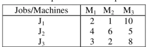
The following example illustrates the use of the initial version of IHSA* to solve the flow-shop problem given in Table 1. For instructional purposes the problem is deliberately simple with only 3 machines and 3 jobs because it is intended to provide readers with an opportunity to become familiar with the algorithm using an example that can be reworked easily by hand.

Table 1: Example of a Flow-shop Problem Jobs/Machines M1 M2 M3

J1 J2 J3

2 1 10 4 6 5 3 2 8

For illustrative purposes only the first search path diagram is presented in Figure 2.

At the start of the search H3 = 26. In total 5 search path diagrams are required to find the optimal sequence J1J2J3 with a minimum makespan of 26. Twenty nodes are expanded, 16 backtracking steps are required, and 43 steps of the algorithm are executed.

3

Modifications to the initial version

of IHSA

*

The first modification determines the best heuristic function to use for a given problem and affects Step 1 of the algorithm. The second modification affects Procedure 1 used in Step 2 and the third modification affects Step 7 and enables multiple optimal solutions to be found when they exist.

3.1

A modification to step 1

In the Appendix a set of 6 heuristic functions are derived for the case of 3 machines and proofs of the admissibility of these functions are presented. It is shown that among this set of 6 heuristic functions the one which

Figure 2: The First Search Path Diagram Using the Initial Version of IHSA*

is admissible and has a value which is closest to the minimum makespan will be the one among H1, H2, and H3 which has the largest value where,

H1 = min[b1 + c1, b2 + c2, …, bn + cn] + _i n

i

a

∑

=1 ,

H2 = min[a1 + u1, a2 + u2, …, an + un] + _i n

i

b

∑

=1

, (5)

H3 = min[a1 + b1, a2 + b2, …, an + bn] + _i n

i

c

∑

=1 ,

where: u1 = min[c2, c3, …, cn]; uk = min[c1, c2, …, ck-1, ck+1, …, cn], for 2 ≤ k ≤ n – 1; and un = min[c1, c2, c3, …, cn-1].

the search since backtracking takes the search back to a previous node and increases the heuristic estimate at that node to a value which is admissible but closer to the minimum time required to complete all of the incomplete jobs on all of the machines.

Consequently, Step 1 in the initial version of IHSA* is modified and becomes:

Step1: At state level 0, from (5), choose the admissible heuristic function among H1, H2, and H3 which has the

largest value and if necessary break ties randomly. In the case where machine Mj dominates the other machines

select Hj. Expand the node identified by the chosen

admissible heuristic function and move to the nodes at state level 1. If more than one node is identified then break ties randomly.

The example in section 4 below illustrates the use of the modification to Step 1 in a simple problem which enables the reader to rework the example by hand. In the Appendix it is shown that in the particular case where machine Mj dominates the other machines then the best admissible heuristic function among H1, H2, and H3 is Hj and it has a value which is greater than the value of either of the other two functions by at least (n – 1)(n – 2) where n is the number of jobs. Thus in the case of a dominant machine in the first step of the algorithm there is no need to calculate each of the values of H1, H2, and H3 in order to choose the one with the largest value. Instead, it is known that it will be Hj if machine Mj is the dominant machine.

In the case where there are m machines and m > 3 it is shown in the Appendix that the best admissible heuristic function to use in the first step of the algorithm is the one among F1, F2, …, Fm which has the largest value and if m = 3 then F1 = H1, F2 = H2, and F3 = H3. Experimental evidence of improvements in performance characteristics of the algorithm which result from using the modification to Step 1 is presented in the Appendix Table A1 and is discussed below in section 5.

3.2

A modification to step 2

The second modification to the initial version of IHSA* concerns the calculation of heuristic estimates at nodes on the search path when the search has commenced. It is based on the principle that when heuristic estimates for the nodes at the same state level are being calculated in Step 2 it is desirable to obtain the largest possible estimate at each of these nodes before selecting the node with the smallest estimate as the node to be expanded. The larger the value of this smallest estimate then the less likely it is that the search will need to backtrack and this is expected to improve the performance characteristics of the algorithm. As noted above, the use of Procedure 1 in Step 2 in the initial version of IHSA* gives a heuristic estimate for a node based on an operation in only one of the cells while operations in the other 2 cells are not taken into account.

The second modification affects Procedure 1 and involves calculating heuristic estimates h1, h2, and h3 at a node for cells 1, 2, and 3, respectively. Then max[h1, h2, h3] is used as the heuristic estimate (h) for the node. This

is done for each node at the current state level and then, as before, in Step 3 the minimum estimate among these estimates identifies the node to be expanded. Consequently, Procedure 1 is replaced by the following Procedure 2:

In Step 2 of the algorithm for a node at the current state level,

(a) For cell 1: If the cell is blank then h1 = 0. Otherwise, h1 is given by (2).

(b) For cell 2: If the cell is blank then h2 = 0. (6) Otherwise, h2 is given by (3).

(c) For cell 3: If the cell is blank then h3 = 0. Otherwise, h3 is given by (4).

Procedure 2 refers to calculations specified in Procedure 1 which incorporate currently the heuristic function H3. However, (2), (3), and (4) are easily changed to incorporate H1 or H2 for problems where one of these functions has been selected using the modification to Step 1 of the algorithm. For example, if H2 is used then (3) and (4) are not changed but (2) becomes,

h= ai + wi + B1; for Oi1 in the not scheduled state, pi1 + wi + bi + B1; for Oi1 in the in-progress state, where, B1 is the sum of the values of bk for all values of k ≠ i such that Ok1 is in the not scheduled state and wi is the smallest value of ck for all values of k ≠ i such that Ok1 is in the not scheduled state.

Procedure 2 produces the same heuristic estimate as Procedure 1 if and only if one of the following 3 conditions is satisfied: h1 = max[h1, h2, h3]; h2 = max[h1, h2, h3] and cell 1 is blank; or h3 = max[h1, h2, h3] and cells 1 and 2 are blank. Under any other conditions Procedure 2 will produce a heuristic estimate at a node which is larger than the estimate given by Procedure 1. Consequently, using Procedure 2 will never produce an estimate that is less than the estimate produced by Procedure 1 and in practice the estimate using Procedure 2 is usually larger and leads to a reduction in backtracking.

Using Procedure 2 in the initial version of IHSA* modifies Step 2 and it becomes:

Step 2: At the current state level if the heuristic estimate of one of the nodes has been updated by backtracking use the updated value as the heuristic estimate for that node and proceed to Step 3. Otherwise, at each node use Procedure 2 to calculate h1, h2, h3 and use max[h1, h2,

h3] as the heuristic estimate for the node.

If there are m machines and m > 3 then there are m cells at each node and an estimate is calculated for each cell by extending (6) and (2), (3), (4) to accommodate the heuristic function Fj (see Appendix) used in Step 1 of the algorithm.

3.3

A modification to step 7

For some problems there are multiple optimal solutions and it is often important in practical situations to be able to find all of the optimal solutions since it may be required to find an optimal solution that also satisfies other criteria. For example, an optimal solution may be sought which also has the least waiting time for jobs that are queuing to be processed.

When IHSA* is implemented there are 2 situations which indicate the possible existence of multiple optimal solutions. The first situation occurs when there is more than 1 node at a state level with the smallest heuristic estimate. In this case the ties are broken randomly and one of the nodes is selected for expansion and the search continues and produces an optimal solution. At the completion of the search returning to that state level and selecting for expansion one of the other nodes which were not selected when the ties were broken may lead to a different optimal solution. The second situation occurs when at the completion of the search for an optimal solution one or more of the nodes at state level 0 has a heuristic estimate that is less than or equal to the minimum makespan. In this case returning to those nodes and beginning the search again may produce different optimal solutions.

The modification to the initial version of IHSA* that enables multiple optimal solutions to be determined affects Step 7. This modification is different from the previous 2 modifications in that it does not improve the performance characteristics of the algorithm but instead it is intended to find multiple optimal solutions if they exist.

Consequently, Step 7 becomes:

Step 7: If f = 0 and h = 0 then an optimal solution has been found. If along the path representing the optimal solution there is a node which was selected for expansion by breaking ties randomly among nodes at the same state level with the same minimum heuristic estimate then return to that state level and repeat from Step 2 ignoring any node that was selected previously for expansion as a result of breaking ties. If any of the values of h at root nodes (state level 0) is less than or equal to the minimum makespan then return to state level 0 and repeat from Step 2 ignoring root nodes that lead to a previous optimal solution. Otherwise, Stop.

4

The final version of IHSA

*

The final version of IHSA* incorporates each of the 3 modifications:

Step1: At state level 0, from (5), choose the admissible heuristic function among H1, H2, and H3 which has the

largest value and if necessary break ties randomly. In the case where machine Mj dominates the other machines

select Hj. Expand the node identified by the chosen

admissible heuristic function and move to the nodes at state level 1. If more than one node is identified then break ties randomly.

Step 2: At the current state level if the heuristic estimate of one of the nodes has been updated by backtracking use

the updated value as the heuristic estimate for that node and proceed to Step 3. Otherwise, at each node use Procedure 2 to calculate h1, h2, h3 and use max[h1, h2,

h3] as the heuristic estimate for the node.

Step 3: At the current state level select the node with the smallest heuristic estimate. If it is necessary then break ties randomly.

Step 4: Calculate f = h + k where h is the smallest heuristic estimate found in Step 3 and k (edge cost) is the time that has elapsed since the preceding state transition occurred.

Step 5: If f > h’, where h’ is the minimum heuristic estimate calculated at the preceding state level, then backtrack to that preceding state level and increase the value of h’ at that preceding node to the current value of f and repeat Step 4 at that node.

Step 6: If f ≤ h’ then proceed to the next state level and repeat from Step 2.

Step 7: If f = 0 and h = 0 then an optimal solution has been found. If along the path representing the optimal solution there is a node which was selected for expansion by breaking ties randomly among nodes at the same state level with the same minimum heuristic estimate then return to that state level and repeat from Step 2 ignoring any node that was selected previously for expansion as a result of breaking ties. If any of the values of h at root nodes (state level 0) is less than or equal to the minimum makespan then return to state level 0 and repeat from Step 2 ignoring root nodes that lead to a previous optimal solution. Otherwise, Stop.

If there are m machines and m > 3 then Steps 1 and Step 2 need to be modified in accordance with the discussion of this case presented in sections 3.1 and 3.2 above.

The simple instructive example which was used to illustrate the initial version of IHSA* (see Table 1) is used again to illustrate the final version of IHSA*. For this problem, from (5), H3 = 26 > H1 = 19 > H2 = 16 and using the modification to Step 1 of the algorithm H3 is used in Step 1 of the algorithm. Since no backtracking is necessary an optimal solution for the problem requires only 1 search path diagram which is shown in Figure 3 where the optimal solution has a minimum makespan of 26 and a job sequence J1, J2, J3. At each node the search path diagram shows the estimates h1, h2, h3 and the heuristic estimate for the node h = max[h1, h2, h3] which result from the use of the modification to Step 2 of the algorithm.

Figure 3: Search Path Diagram Using the Final Version of IHSA*

node at which job J3 is scheduled on machine M1 is expanded. This gives a second optimal solution where the job sequence is J1, J3, J2.

5

Experimental evidence of

improvements in performance

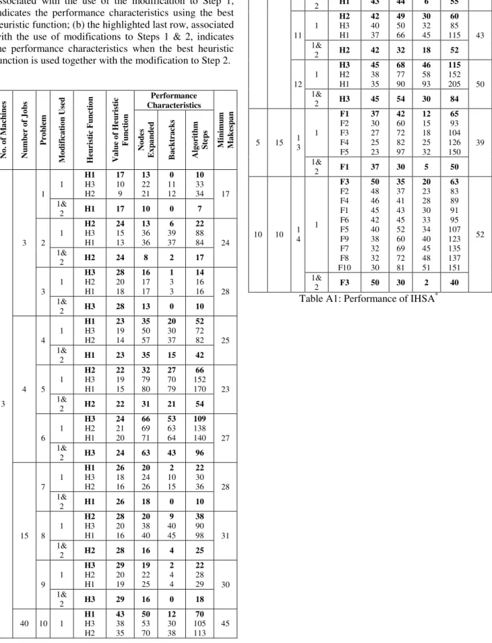
Experimental evidence of improvements in performance characteristics of IHSA* using the modifications to Steps 1 and 2 is presented in Appendix Table A1. The characteristics considered are: the number of nodes expanded; the number of backtracking steps required; and the number of steps of the algorithm executed.

In total 14 problems are considered involving: 3, 5 and 10 machines; and 3, 4, 10, 15, and 40 jobs. Each problem involving 3 machines was solved using the heuristic functions H1, H2, and H3 in (5) which are the same as F1, F2, and F3, respectively, when m = 3. Problems involving 5 and 10 machines were solved using their corresponding heuristic functions F1, F2, F3, F4, F5 and F1, F2, F3, …, F10, respectively. The solutions enabled improvements in the performance characteristics resulting from the use of only the modification to Step 1 to be assessed. In addition, for each problem the solution was obtained using the modification to Step 1 together with the modification to Step 2. The performance

characteristics associated with each of these solutions enabled an assessment of any further improvements in performance characteristics resulting from the inclusion of the modification to Step 2.

From Table A1 it is seen that for each problem regardless of the number of jobs and machines the modification to Step 1, which involves using the heuristic function with the largest value in Step 1, leads to improvements in all of the performance characteristics. Furthermore, in each problem using the modification to Step 1 together with the modification to Step 2, which affects the calculation of heuristic estimates as the search progresses, leads to further improvements in the performance characteristics.

6

Conclusion

Three modifications to the initial version of a new intelligent heuristic search algorithm (IHSA*) have been described. The algorithm guarantees an optimal solution for flow-shop problems involving an arbitrary number of jobs and machines provided the job sequence is the same on all of the machines.

The first modification affects Step 1 of the algorithm and concerns the choice of an admissible heuristic function which is as close as possible to the minimum makespan for the problem. For problems with an arbitrary number of jobs and 3 machines (M1, M2, M3) a set of 6 possible functions is derived (H1, H2, …, H6) and their admissibility is proved. It is shown that the function which has a value that is closest to the minimum makespan and is the best function to use in Step 1 of the algorithm is the function among H1, H2, and H3 which has the largest value. In the particular case where one of the machines (Mj) dominates the other 2 machines the best function is Hj and there is no need to calculate the values of the other 2 functions. Furthermore, its value is greater than the value of either of the other 2 functions by at least O(n2) where n is the number of jobs. More generally, for problems with more than 3 machines (M1, M2, …, Mm) the best admissible heuristic function to use is the one among F1, F2, …, Fm with largest value and if machine Mj dominates the other machines then Fj is the best heuristic function. The proofs of these more general results may be obtained following the methods used in the proofs presented in the Appendix of the corresponding results for H1, H2, and H3.

The first and second modifications ensure that at the start of the search and as the search progresses heuristic estimates are admissible and are as close as possible to the minimum time needed to complete all of the incomplete operations on all of the machines. This reduces the chance that the search will backtrack and improves the performance characteristics of the algorithm. Experimental evidence from problems involving various numbers of machines and jobs indicates that although the first modification produces improvements in performance characteristics of the algorithm these improvements are enhanced when the second modification is included.

The third modification relates to Step 7 of the algorithm and concerns problems where there are multiple optimal solutions. It enables all of the optimal solutions to be found and this is convenient for situations where additional criteria may need to be satisfied by an optimal solution.

This article has focussed on describing the development of the final version of IHSA*. However, there are several areas for future investigation including a comparison of the performance of the algorithm with other methods such as branch- and-bound methods and methods for pruning the search tree in order to improve memory management during implementation.

References

[1] Blum, C., Roli, A. “Metaheuristics in combinatorial optimization: overview and conceptual comparison,” ACM Comput. Surv., 35, 2003, 268-308.

[2] Chen, C.L., Neppalli, R.V., Aljaber, N. “Genetic algorithms applied to the continuous flow shop problem,” Computers and Industrial Engineering 30: (4), 1996, 919-929.

[3] Cleveland, G.A., Smith, S.F. “Using genetic algorithms to schedule flow shop,” Proceedings of 3rd Conference on Genetic Algorithms, Schaffer, D.(ed.), San Mateo: Morgan Kaufmann Publishing, 1989, 160-169.

[4] Conway, R.W., Maxwell, W.L., Miller, L.W. Theory of scheduling, Addison-Wesley, Reading Massachusetts, 1967.

[5] Eitler, O., Toklu, B., Atak, M., Wilson,J. “A genetic algorithm for flowshop scheduling problems,” J. Oper. Res. Soc., 55, 2004, 830-835.

[6] Fan, J.P.-O. “The development of a heuristic search strategy for solving the flow-shop scheduling problem,” Proceedings of the IASTED International Conference on Applied Informatics, Innsbruck, Austria, 1999, 516-518.

[7] Fan, J.P.-O. “An intelligent search strategy for solving the flow-shop scheduling problem,” Proceedings of the IASTED International Conference on Software Engineering, Scottsdale, Arizona, USA, 1999, 99-103.

[8] Fan, J.P.-O. An intelligent heuristic search method for flow-shop problems, doctoral dissertation, University of Wollongong, Australia, 2002.

[9] Framinan, J.M, Ruiz-Usano, R., Leisten, R. “Sequencing CONWIP flow-shops: analysis and heuristic,” Int. J. Prod. Res., 39, 2001, 2735-2749. [10] Gheoweth, S.V., Davis, H.W. “High performance

A* search using rapidly growing heuristics,” Proceedings of the International Joint Conference on Artificial Intelligence, Sydney, Australia, 1991, 198-203.

[11] Grabowski, J., Wodecki, M. “A very fast tabu search algorithm for the permutation flowshop problem with makespan criterion,” Comput. Oper. Res., 31, 2004, 1891-1909.

[12] Hart, P.E., Nilsson, N.J., Raphael, B. “A formal basis for the heuristic determination of minimum cost paths,” IEEE Transactions on Systems Science and Cybernetics, Vol. SSC-4: (2), 1968, 100-107. [13] Hong, T.P., Chuang, T.N. “Fuzzy scheduling on

two-machine flow shop,” Journal of Intelligent & Fuzzy Systems, 6: (4), 1998, 471-481.

[14] Hong, T.P., Chuang, T.N. “Fuzzy CDS scheduling for flow shops with more than two machines,” Journal of Intelligent & Fuzzy Systems, 6: (4), 1998, 471-481.

[15] Hong, T.P., Chuang, T.N. “Fuzzy Palmer scheduling for flow shops with more than two machines,” Journal of Information Science and Engineering, Vol.15, 1999, 397-406.

[16] Hong, T.P., Wang, T.T. “A heuristic Palmer-based fuzzy flexible flow-shop scheduling algorithm,” Proceedings of the IEEE International Conference on Fuzzy Systems, Vol. 3, 1999, 1493-1497. [17] Hong, T.P., Huang, C.M., Yu, K.M. “LPT

scheduling for fuzzy tasks,” Fuzzy Sets and Systems, Vol. 97, 1998, 277-286.

[18] Hong, T.P., Wang, C.L., Wang, S.L. “A heuristic Gupta-based flexible flow-shop scheduling algorithm,” Proceedings of the IEEE International Conference on Systems, Man and Cybernetics, Vol. 1, 2000, 319-322.

[19] Ignall, E., Schrage, L.E. “Application of the branch and bound technique to some flow shops scheduling problems,” Operations Research, Vol. 13: (3), 1965, 400-412.

[20] Johnson, S.M. “Optimal two- and three-stage production schedules with setup times included,” Naval Research Logistics Quarterly, 1: (1), 1954, 61-68.

[21] Kamburowski, J. “The nature of simplicity of Johnson’s algorithm,” Omega-International Journal of Management Science, 25: (5), 1997, 581-584. [22] Korf, R.E. “Depth-first iterative-deepening: an

optimal admissible tree search,” Artificial Intelligence, Vol. 27, 1985, 97-109.

[23] Korf, R.E. “Iterative-deepening A*: an optimal admissible tree search,” Proceeding of the 9th International Joint Conference on Artificial Intelligence, Los Angeles, California, 1985, 1034-1036.

[25] Korf, R.E. “Linear-space best-first search,” Artificial Intelligence, 62: (1), 1993, 41-78.

[26] Lai, T.C. “A note on heuristics of flow-shop scheduling,” Operations Research, 44: (6), 1996, 648-652.

[27] Lee, G.C., Kim, Y.D., Choi, S. W. “Bottleneck-focused scheduling for a hybrid flow-shop,” Int. J. Prod. Res., 42, 2004, 165-181.

[28] Liu, B., Wang, L., Jin, Y-H. “An effective PSO-based memetic algorithm for flow shop scheduling, “IEEE T. Syst. Man. CY. B.,” 37, 2007, 18-27. [29] Lomnicki, Z. “A branch and bound algorithm for the

exact solution of three machine scheduling problem,” Operational Research Quarterly, 16: (1), 1965, 89-100.

[30] McMahon, C.B., Burton, P.G. “Flow-shop scheduling with the branch and bound method,” Operations Research, 15: (3), 1967, 473-481. [31] Nawaz, M., Enscore Jr. E., Ham, I. “A heuristic

algorithm for the m-machine, n-job flow-shop sequencing problem,” Omega-Int. J. Manage. S., 11, 1983, 91-95.

[32] Ogbu, F.A., Smith, D.K. “The application of the simulated annealing algorithm to the solution of the n/m/Cmax flowshop problem,” Comput. Oper. Res., 17, 1990, 243-253.

[33] Onwubolu, G.C., Davendra, D. “Scheduling flow-shops using differential evolution algorithm,” Eur. J. Oper. Res., 171, 2006, 674-692.

[34] Osman, I., Potts, C. “Simulated annealing for permutation flow shop scheduling,” OMEGA, 17, 1989, 551-557.

[35] Pan, C.H. “A study of integer programming formulations for scheduling problems,” International Journal of System Science, 28: (1), 1997, 33-41.

[36] Pan, C.H., Chen, J.S. “Scheduling alternative operations in two-machine flow-shops,” Journal of the Operational Research Society, 48: (5), 1997, 533-540.

[37] Ravendran, C. “Heuristic for scheduling in flowshop with multiple objectives,” Eur. J. Oper. Res., 82, 1995, 540-555.

[38] Ruiz, R., Maroto, C., Alcaraz, J. “Two new robust genetic algorithms for the flowshop scheduling problem,” Omega-Int. J. Manage. S., 34, 2006, 461-476.

[39] Stutzle, T. “Applying iterated local search to the permutation flowshop problem,” AIDA-98-04, TU Darmstadt, FG Intellektik, 1998.

[40] Taillard, E. “Some efficient heuristic methods for the flow shop sequencing problem,” Eur. J. Oper. Res., 47, 1990, 65-74.

[41] Taillard, E. “Benchmarks for basic scheduling problems,” Eur. J. Oper. Res., 64, 1993, 278-285. [42] Wang, C.G., Chu, C.B., Proth, J.M. “Efficient

heuristic and optimal approaches for N/2/F/SIGMA-C-I scheduling problems,” International Journal of Production Economics, 44: (3), 1996, 225-237.

[43] Ying, K.C., Liao, C.J. “An ant colony system for permutation flow-shop sequencing,” Comput. Oper. Res., 31, 2004, 791-801.

[44] Zamani, M.R., Shue, L.Y. “Developing an optimal learning search method for networks,” Scientia Iranica, 2: (3), 1995, 197-206.

[45] Zamani, R., Shue, L.Y. “Solving project scheduling problems with a heuristic learning algorithm,” Journal of the Operational Research Society, 49: (7), 1998, 709-716.

[46] Zamani, M.R. “A high performance exact method for the resource-constrained project scheduling problem,” Computers and Operations Research, 28, 2001, 1387-14.

[47] Zobolas, G.I., Tarantilis, C.D., Ioannou, G. “Minimizing makespan in Permutation Flow Shop scheduling problems using a hybrid metaheuristic algorithm,” Computers and Operations Research, 2008, doi:10.1016/j.cor.2008.01.007.

Appendix

Derivation of heuristic functions

The purpose is to develop heuristic functions suitable for use in IHSA*. In each case the objective is to develop a function which underestimates the minimum makespan (i.e. admissible). Six functions are developed and the proof of their admissibility is presented in the next section.

From Figure 1, S(φst ) ≥ max [bt +, as + i n

i

b

∑

=1

] and

T(φst ) ≥ max [S(φst ) + ct , as + bs + _i n

i

c

∑

=1

] which means that:

T(φst ) ≥ as + bs + i n

i

c

∑

=1

or, (A1)

T(φst ) ≥ S(φst ) + ct ≥ bt + ct + i n

i

a

∑

=1

or, (A2)

T(φst ) ≥ as + ct + i n

i

b

∑

=1

. (A3) From (A1) two heuristic functions H3 and H6 are

proposed:

H3 = min[a1 + b1, a2 + b2, …, an + bn] + _i n

i

c

∑

=1

and

H6 = min[a1, a2, …, an] + min[b1, b2, …, bn] + _i n

i

c

∑

least _i n

i

c

∑

=1

units of time. Since min[a1 + b1, a2 + b2, …, an + bn] ≥ min[a1, a2, …, an] + min[b1, b2, …, bn] it follows that H3 ≥ H6, which is therefore also a plausible heuristic function.

H1 and H5 are derived from (A2):

H1 = min[b1 + c1, b2 + c2, …, bn + cn] + _i n

i

a

∑

=1

and

H5 = min[b1, b2, …, bn] + min[c1, c2, …, cn] + _i n

i

a

∑

=1 . The rationale for the development of H1 is: select the job which requires the least total amount of time on machines M2 and M3 (i.e. min[b1 + c1, b2 + c2, …, bn + cn] units of time) and suppose that it is placed last in the job sequence which means that the earliest time that it can start on M2 is after _i

n

i

a

∑

=1

units of time. Since min[b1 + c1, b2 + c2, …, bn + cn] ≥ min[b1, b2, …, bn] + min[c1, c2, …, cn] it follows that H1 ≥ H5, which is therefore also a plausible heuristic function.

H2 and H4 are derived from (A3):

H2 = min[a1 + u1, a2 + u2, …, an + un] + _i n

i

b

∑

=1

and

H4 = min[a1, a2, …, an] + min[c1, c2, …, cn] + _i n

i

b

∑

=1 , where: u1 = min[c2, c3, …, cn]; uk = min[c1, c2, …, ck-1, ck+1, …, cn] for 2 ≤ k ≤ n – 1; and un = min[c1, c2, c3, …, cn-1]. The rationale for the development of H2 is: consider each job in turn and suppose that it is placed first in the job sequence and then from among all of the other jobs select the one which requires the least amount of time on M3. Now for each pair of jobs selected in this manner determine the pair that gives the least total time on M1 and M3. This total time plus the minimum total time required to finish all of the jobs on M2 is the value of H2. Also, min[a1 + u1, a2 + u2, …, an + un] ≥ min[a1, a2, …, an] + min[u1, u2, …, un] = min[a1, a2, …, an] + min[c1, c2, …, cn] and it follows that H2 ≥ H4, which is therefore also a plausible heuristic function.

Admissibility

Results and selected proofs related to the admissibility of the heuristic functions H1,

H2, H3, H4, H5, and H6 are presented: R₁. _{H3 ≥ H6 and both are admissible.}

R₂. _{H2 ≥ H4 and both are admissible.} R₃. _{H1 ≥ H5 and both are admissible.}

Only a proof for R2 _{is given since the remaining} proofs may be constructed in the same manner.

From (A3), T(φst) ≥ as + ct + i n

i

b

∑

=1

for s, t = 1, 2, …, n with s ≠ t and so in particular, T(φ1t) ≥ a1 + ct +

i n

i

b

∑

=1

, T(φ2t) ≥ a2 + ct + _i n

i

b

∑

=1

, …, T(φnt) ≥ an + ct +

i n

i

b

∑

=1 .

Hence, if T*(φst) denotes the earliest time at which any job sequence which starts with job Js is completed on M3 then T*(φ1t) ≥ min[a1 + c2, a1 + c3, …, a1 + cn] + i

n

i

b

∑

=1 ,

T*(φ2t) ≥ min[a2 + c1, a2 + c3, …, a2 + cn] + i n

i

b

∑

=1

, …, T*(φnt) ≥ min[an + c1, an + c2, …, an + cn-1, …, an + cn ] +

i n

i

b

∑

=1

and the minimum makespan T* = min[T*(φ1t), T*(φ2t), …, T*(φnt)] ≥ min[a1 +u1, a2 + u2, …, an + un] +

i n

i

b

∑

=1

= H2 ≥ min[a1, a2, …, an] + min[c1, c2, …, cn] +

i n

i

b

∑

=1

= H4. Consequently, H2 ≥ H4 and both are admissible.

From the results R1, R2, and R3 it is seen that the heuristic functions H1, H2, H3, H4, H5, and H6 are all admissible. However, in order to select the heuristic function among these that is the closest in value to the minimum makespan (i.e. the best to use in Step1 of IHSA*) the choice should be made from among only H1, H2, and H3 because the function among these 3 which has the largest value is admissible and has a value which is larger than any of the other 5 admissible functions. Consequently, in Step1 of IHSA* the values of H1, H2, and H3 are calculated and the function with the largest value is selected for use.

Dominance

Machine M1 dominates the other 2 machines if min[a1, a2, …, an] ≥ max[b1, b2, …, bn] and min[a1, a2, …, an] ≥

max[c1, c2, …, cn] and similar definitions apply if machine M2 or machine M3 is dominant.

In the case of a dominant machine results R5, R6, and R7 identify immediately which heuristic function among H1, H2, and H3 has the largest value and is the best to use in IHSA*. Also, from R8 it is seen that the best heuristic function has a value which is greater than the value of either of the other functions by O(n2) where n is the number of jobs.

R5. _{If machine M1 dominates then H1 is the heuristic} function with the largest value,

R6. _{If machine M2 dominates then H2 is the heuristic} function with the largest value,

R7. _{If machine M3 dominates then H3 is the heuristic} function with the largest value.

The proofs for R5 and R8 are given noting that proofs for the other results may be constructed in the same manner. Throughout these proofs min(ai) = min[a1, a2, …, an], min(bi) = min[b1, b2, …, bn], min(ci) = min[c1, c2, …, cn], max(ai) = max[a1, a2, …, an], max(bi) = max[b1, b2, …, bn], and max(ci) = max[c1, c2, …, cn].

Suppose machine M1 dominates and for i = 1, 2, 3, …, n: ai ∈ [r1, r1 + w –1]; bi ∈ [s1, s1 + l –1]; and ci ∈ [t1, t1 + d –1] are distinct non negative integers from intervals of widths w, l, and d, respectively, each greater than or equal to n (the number of jobs).

It follows that the minimum values of i n

i

a

∑

=1

, i

n i

b

∑

=1 , i n i

c

∑

=1

are nr1 + 0.5n(n – 1), ns1 + 0.5n(n – 1), and nt1 + 0.5n(n – 1), respectively, and when these minimum values are attained min(ai) = r1, min(bi) = s1, min(ci) = t1, max(ai) = r1 + n – 1, max(bi) = s1 + n – 1, and max(ci) = t1 + n –1 for i = 1, 2, 3, …, n.

Also, the maximum values of i n

i

a

∑

=1

, i

n i

b

∑

=1 , i n i

c

∑

=1

are n(r1 + w) – 0.5n(n + 1), n(s1 + l) – 0.5n(n + 1), and n(t1 + d) – 0.5n(n + 1), respectively, and when these maximum values are attained min(ai) = r1 + w – n, min(bi) = s1 + l – n, min(ci) = t1 + d – n, max(ai) = r1 + w – 1, max(bi) = s1 + l – 1, max(ci) = t1 + d – 1.

Now, H1 = min[b1 + c1, b2 + c2, …, bn + cn] + _i n i

a

∑

=1

≥ min(bi) + min(ci) + min( _i n

i

a

∑

=1

) (A4) and similarly,

H2 ≤ max(ai) + max(ci) + max( _i n

i

b

∑

=1

) (A5)

and H3 ≤ max(ai) + max(bi) + max( _i n

i

c

∑

=1

). (A6) If (A4), (A5), (A6) are all true then,

H1 ≥ s1 + l – n + t1 + d – n + nr1 + 0.5n(n – 1), (A7) H2 ≤ r1 + n – 1 + t1 + d – 1 + n(s1 + l) – 0.5n(n + 1), (A8)

H3 ≤ r1 + n – 1 + s1 + l – 1 + n(t1 + d) – 0.5n(n + 1). (A9) From (A7) and (A8),

s1 + l – n + t1 + d – n + nr1 + 0.5n(n – 1) – r1 – n + 1 – t1 – d +1 – n(s1 + 1) + 0.5n(n + 1) = s1 – ns1 + l – nl + nr1 – r1 + n2 – 3n + 2 = (n – 1)[r1 – (s1 + l) + n – 2] ≥ (n – 1)(n – 2) ≥ 0 , for n ≥ 2, and so H1 is greater than H2 by a value which is at least (n – 1)(n – 2), for n ≥ 3.

In a similar manner it follows from (A7) and (A9) that H1 is greater than H3 by a value which is at least (n – 1)(n – 2), for n ≥ 3 and this completes the proof of R5 and R8.

The best admissible heuristic function for an

arbitrary number of machines

For the case where there are more than 3 machines there is a need to change the notation used previously to represent the time that each operation Oi,j requires on each machine so that ti,j is the number of units of time required by job Ji on machine Mj.

If there are m machines then the best admissible heuristic function will be the one with the largest value among the set of m functions F1, F2, F3, …, Fm where,

Fj = min[ _i

m i

t

1, 2

∑

= , _i m i

t2, 2

∑

=

, …, _ni

m i t , 2

∑

=

] + _,1 1 i n i t

∑

=

, for j=1,

min[ 1 , , 1 1 1 j i j i u t +

∑

− = , 2 , , 2 1 1 j i j i u t +

∑

− = , …, n j i n j i u

t_{, ,}

1 1 +

∑

− = ] + j i n i t, 1

∑

=

, for 2 ≤ j ≤ m,

where, for 2 ≤ j ≤ m – 1, min[

i m

j i

t_2, 1

∑

+ = , i m j i

t_3, 1

∑

+ = , …, i n m j i t _, 1

∑

+ =

], for k = 1,

uj,k = min[

i m

j i

t_1, 1

∑

+ = , i m j i

t2, 1

∑

+ = , …, i k m j i

t _1, 1 − + =

∑

, i k m j i

t _1, 1 + + =

∑

, …, ni m j i

t

_, 1

∑

+ =

], for 2 ≤ k ≤ n – 1,

min[

i m

j i

t_1, 1

∑

+ = , i m j i

t_2, 1

∑

+ = , …, i n m j i

t _1, 1

− + =

∑

], for k = n,

and um,k = 0, for k = 1, 2, 3, …, n.

For a problem with m machines where m > 3 and the job sequence is the same on each machine the function among F1, F2, F3, …, Fm with the largest value is selected in Step 1 of IHSA*.

Experimental evidence of improvements in

performance characteristics

Table A1: Performance of IHSA*: Modification to Step 1 compared to Modifications to Steps 1 and 2.

Note: For each problem: (a) the highlighted first row, associated with the use of the modification to Step 1, indicates the performance characteristics using the best heuristic function; (b) the highlighted last row, associated with the use of modifications to Steps 1 & 2, indicates the performance characteristics when the best heuristic function is used together with the modification to Step 2.

N o . o f M a ch in es N u m b er o f J o b s P ro b le m M o d if ic a ti o n U se d H eu ri st ic F u n ct io n V a lu e o f H eu ri st ic F u n ct io n Performance Characteristics M in im u m M a k es p a n N o d es E x p a n d ed B a ck tr a ck s A lg o ri th m S te p s 3 3 1 1 H1 H3 H2 17 10 9 13 22 21 0 11 12 10 33

34 17

1&

2 H1 17 10 0 7

2 1 H2 H3 H1 24 15 13 13 36 36 6 39 37 22 88

84 24

1&

2 H2 24 8 2 17

3 1 H3 H2 H1 28 20 18 16 17 17 1 3 3 14 16

16 28

1&

2 H3 28 13 0 10

4 4 1 H1 H3 H2 23 19 14 35 50 57 20 30 37 52 72

82 25

1&

2 H1 23 35 15 42

5 1 H2 H3 H1 22 19 15 32 79 80 27 70 79 66 152

170 23

1&

2 H2 22 31 21 54

6 1 H3 H2 H1 24 21 20 66 69 71 53 63 64 109 138

140 27

1&

2 H3 24 63 43 96

15 7 1 H1 H3 H2 26 18 16 20 24 26 2 10 15 22 30

36 28

1&

2 H1 26 18 0 10

8 1 H2 H3 H1 28 20 16 20 38 40 9 40 45 38 90

98 31

1&

2 H2 28 16 4 25

9 1 H3 H2 H1 29 20 19 19 22 25 2 4 4 22 28

29 30

1&

2 H3 29 16 0 18

40 10 1

H1 H3 H2 43 38 35 50 53 70 12 30 38 70 105 113 45 N o . o f M a ch in es N u m b er o f J o b s P ro b le m M o d if ic a ti o n U se d H eu ri st ic F u n ct io n V a lu e o f H eu ri st ic F u n ct io n Performance Characteristics M in im u m M a k es p a n N o d es E x p a n d ed B a ck tr a ck s A lg o ri th m S te p s 1&

2 H1 43 44 6 55

11 1 H2 H3 H1 42 40 37 49 50 66 30 32 45 60 85

115 43

1&

2 H2 42 32 18 52

12 1 H3 H2 H1 45 38 35 68 77 90 46 58 93 115 152

205 50

1&

2 H3 45 54 30 84

5 15 1

3 1 F1 F2 F3 F4 F5 37 30 27 25 23 42 60 72 82 97 12 15 18 25 32 65 93 104 126 150 39 1&

2 F1 37 30 5 50

10 10 1₄ 1 F3 F2 F4 F1 F6 F5 F9 F7 F8 F10 50 48 46 45 42 40 38 32 32 30 35 37 41 43 45 52 60 69 72 81 20 23 28 30 33 34 40 45 48 51 63 83 89 91 95 107 123 135 137 151 52 1&

2 F3 50 30 2 40