Order Selection of Spatial and
Temporal Autoregressive Models
with Errors in Variables
Mauro Coli, Lara Fontanella and Luigi Ippoliti
Department of Quantitative Method and Economic Theory, University “G. D’Annunzio”, Chieti, Italy
In this paper we consider the issues involved in model order selection for processes observed with additive Gaussian noise. In particular, we discuss conditional maximum likelihood estimation of noisy autoregressive models and provide an estimator that takes care of the observational noise. The estimator is weakly consistent, can be computed in only O(n) steps and can be used
in the automatic model identification phase. Using information criteria, an extensive simulation study shows the results of order selection in the context of time and spatial series analysis.
Keywords: autoregressive processes, information crite-ria, conditional maximum likelihood, image analysis.
1. Introduction
Inference on temporal, spatial and spatio-tem-poral autoregressive models, are usually carried out conditionally on a previously selected lag order 5], 6]. In many cases the lag order
se-lection is carried out using several information criteria which have relative advantages depend-ing upon the situation in which they are used. There has been considerable development dur-ing the last decade on the question of time series model selection. For a review see for example 4]. On the other hand, the literature on
spa-tial model selection is sparse and exceptions are the papers 11]and 16]. In this article we are
concerned with the model order selection prob-lem of a temporal or spatial autoregressive(AR)
processXthat is not observed directly. Instead, we assume the analyst observes the process Y such that
Y =X+η (1)
whereηis a white noise with varianceσ2
η, inde-pendent ofX. Although at a first sight it could appear restrictive, the hypothesis thatXmay be represented by AR models permits to overcome the computational burden which is usually en-countered with huge data sets or when a moving-average (MA)component is considered in the
model. In fact, apart from the univariate case where the convergence of the maximum likeli-hood function may not be attained at all 18], it
is known that in the multivariate case, in addi-tion to requiring causality and invertibility, the consideration of the MA component needs fur-ther assumptions which may suggest to fit only vector AR models 17]. Thus, all the
aforemen-tioned problems might partially explain why there have been only a few accounts in the lit-erature of studies involving ARMA or VARMA order selection procedures.
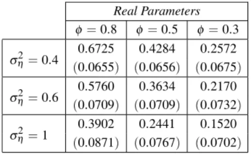
To give insights into the importance of how the signal parameters estimation might be affected by an additive Gaussian error we present in the context of time series analysis, a simple exam-ple regarding a zero mean AR(1) process 5].
In particular, to give a flavour of types of be-haviour of the Ordinary Least Square (OLS)
estimator, Table 1 shows the results of a set of simulations on 500 samples generated with pa-rametersn=200,φ =0:3, 0:5, 0:8,σ
2
η =0:4,
0:6, 1 andσ
2
ε = 1; wherenis the sample size,
φ is the autoregressive parameter and σ2
ε the variance of the driving noise.
Real Parameters
φ=0:8 φ=0:5 φ=0:3
0:6725 0:4284 0:2572 σ2
η=0:4
(0:0655) (0:0656) (0:0675)
0:5760 0:3634 0:2170 σ2
η=0:6
(0:0709) (0:0709) (0:0732)
0:3902 0:2441 0:1520 ση2=1
(0:0871) (0:0767) (0:0702)
Table 1.The means and standard errors(in brackets)of
the OLS estimates of an AR(1)+Noise model.
noise variances, SNR) decreases. However,
such a result is not surprising since the introduc-tion of the observaintroduc-tional noise affects the corre-lation structure of the original process. This can be easily shown for the AR(1)+Noise model.
In fact, since Y is the sum of two independent stationary components, we have that
γy(h)= 8 > > > <
> > > :
σ2
ε 1;φ
2 +σ
2
η forh=0
φh
1;φ
2
σ2
ε forh>0
whereγy(h) = Cov YtYt ;h
],his the temporal
lag and t the discrete index of times. Con-sequently, the autocorrelation function of the observed process is
ρy(h)=
γy(h)
γy(0) =
1+
σ2
η
σ2
ε
(1;φ
2
)
;1
φh
that shows that the processYtis not AR(1)
un-lessσ2
η =0.
Actually, the addition of white noise to an ARMA(mq)process was discussed in 5]. In
general, if m > q, and the process is observed
with error, the resulting observed process is an ARMA(mm) process. The resulting 2m
pa-rameters are a function of the original m+ q
parameters plus the variance of the observa-tional noise. A point worth noting is that the inclusion of the observational error is some-times related to the opportunity to find a more parsimonious model than simply fitting ARMA processes. This is particularly evident for the autoregressive case. In fact, provided the un-derlying process Xt is pure autoregressive —
AR(m);, it is only necessary to estimatem+1
parameters rather than 2m parameters for an ARMA(mm)process.
A natural way of estimating them+1
parame-ters isviaKalman filter 12]that directly allows
to take into account the presence of a measure-ment noise. However, out of the state space form, as we have seen in Table 1, a direct ap-plication of the OLS estimator leads to biased results which alter the one-step ahead prediction error variance.
The purpose of this paper is to propose an OLS estimator that, taking into account the presence of the observational error, can be used as aquick tool for autoregressive model order selection. The paper is outlined as follows. In Section 2 we present the spatial and temporal autore-gressive models as well as the Adjusted Least Square estimator(ALSE)that takes into account
the presence of an external source of error. The problem of model identification involving order selection and the information criteria used in the paper are described in Section 3. Performance of the methods discussed in Sections 2 and 3 is the principal subject of a simulation exercise, the design of which is the main component of Section 4. Finally, in Section 5 we conclude the paper with a discussion.
2. Models and Conditional Maximum Likelihood Estimation
In the framework of temporal and spatial ana-lysis, we investigate two different models.
2.1. Temporal Autoregressive Models
In this case we consider a zero-mean autore-gressive process of orderm 5], given by
m
X
j=0
φjXt;j
=εt φ0 =1 (2)
wheremis unknown,φj,j = 1:::m, are real
parameters such that all the roots of the polyno-mial
m
X
j=0
φjzj =0
lie outside the unit circle, andεt is a Gaussian
white noise process with varianceσ2
this context, several information criteria may be used to pick the lag order of the model.
2.2. Gauss Markov Random Fields
They are widely used as models in spatial ana-lysis of lattice data 6], 9], 7]. Because of the
strong association to image analysis we shall mainly think of the spatial sites as pixels of a
(RC)lattice. Thus, we say that the grey levels
are distributed according to a zero-mean Gauss Markov Random Field(GMRF)if the
distribu-tion ofXis multivariate normal with conditional means and conditional variances
E(XijXj:j2δi)= X
j2δi
βijxj
(3)
Var(XijXj :j2δi)=τ
2
(4)
where δi is the set of neighbors of pixel i(not
including i). Here x = (x1x2:::xn)
T is
a n;vector of grey-levels at pixel (ij), (i =
1:::R;j=1:::C). Note thatn=(RC)
and that the vectorxcontains the pixels in raster scan order-stacking the top row of the image, then the second row, etc. Specification of the model consists of specifying both the dimen-sion of the parameter vector β and the neigh-borhood system δi. In this case, two models
are distinct if their parameter spaces have dif-ferent dimensions, or they are associated with different neighborhood systems or both. To this
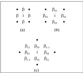
Fig. 1.Neighborhood systems and spatial interaction parameters of a GMRF.
purpose, Figure 1 serves to illustrate the model selection problem.
As it can be seen, the model depicted in Fig-ure 1(a)denotes a first order isotropic GMRF
with single parameterβ. In this case, each site has four neighbours. For the model in Figure 1(b), every site has again four nearest
neigh-bours; however, different parameters β01 and β10 are used for horizontal and vertical pairs
interactions. Finally, Figure 1(c)denotes a
sec-ond order GMRF where the neighbourhood sys-tem has an expanded graph which includes also the diagonal elements(and parameters) in the
southeast and northeast directions. Thus, since the impact of a specification error onto the qual-ity of standard estimation procedures is serious 10], in this case automatic selection criteria can
also be helpful when different models seem vi-able to fit the data.
2.3. TheALSEEstimator
In this section we present an estimator of model parameters that can be used to drive the auto-matic model order selection phase when the data are corrupted by a measurement error.
For the sake of simplicity, we describe the method for the temporal case, but the extension to the spatial case is straightforward 9].
Provided the order,m, of the process is known, the exact log-likelihood function for the pro-cess in (2), can be accomplished numerically
to obtain the maximum likelihood estimates of the parameters. In contrast, conditional on the firstmobservations, the log-likelihood assumes a simpler form and it is easy to show 12]that
the conditional maximum likelihood estimates
ˆ
φ =
X
t
˜ x0
tx˜t
;1
X
t
˜ xtxt
(5)
can be obtained as an OLS regression ofxt on
its own m lagged values placed in the vector ˜
xt. Notice that for the GMRF model the least
squares estimator is better known as maximum Pseudo-Likelihood estimator 3]. However, as
we have shown in the preceding section for the noisy case, a crude and direct application of this estimator leads to biased results. In order to obtain an estimator which takes care of the noise, let us specify ˜yt=x˜t+η˜t, where ˜ηt
observational noise. In this case, considering that X t ˜ y0
ty˜t= X
t
(x˜t+η˜t) 0
(x˜t+η˜t)
= X
t
(x˜ 0
tx˜t)+2 X
t
(x˜ 0
tη˜t)+ X
t
(η˜ 0
tη˜t)
we can use the properties of the moment esti-mators to show that
1 n
X
t=1 (x˜
0
tη˜t)=Op(n ;1=2
)
1 n
X
t
(η˜ 0
tη˜t)=σ
2
ηIm+Op(n ;1=2
) (6)
whereImis the(mm)identity matrix. Finally,
given that 1 n
X
t
(y˜tyt)=
1 n
X
t=1 (x˜
0
tx˜t)+σ
2
ηIm+Op(n ;1=2
)
(7)
it follows that substituting the large sample ap-proximations suggested by(6)and(7)into(5),
we have the Adjusted Least Square Estimator
(ALSE)based on the noisy series
˜ φ = X t ˜ y0
ty˜t;nσ
2
ηIm
;1 X t ˜ ytyt
(8)
Furthermore, since 1
n
X
t
y2t ;
1 n
X
t
x2t =σ
2
η+Op(n ;1=2
)
it is straightforward to show that the Adjusted estimate of the residual variance is
˜ σ2 = 1 n X t
(yt;
˜ φ0
˜ yt)
2
;σ
2
η(1+
˜ φ0˜
φ) (9)
whereσ2
η(1+φ˜ 0φ˜
)is the adjustment which takes
care of the noise.
Finally, notice that the estimator isweakly con-sistentforφ. In fact, from model assumptions,
(6),(7)and(8), it follows that
˜
φ =
ˆ
φ +Op(n ;1=2
) (10)
However, it is well known that the OLS is a consistent estimator forφ under the noise free model, i.e.
ˆ
φ =φ +op(1)
hence, from(10)we have that
˜
φ =φ +op(1)
as required. Thus, this results mean that the estimator is appropriate for large series.
3. Model Order Selection Using Information Criteria
Model identification involving order- selection criteria is usually based on the minimization of a loss function of the following form
H()+P(nm) (11)
where P(nm) is a nonnegative random
vari-able depending directly on sample sizenand the number of estimated parametersm of the can-didate model. In practice,P(nm)measures the
complexity of the candidate model and serves as a penalty term for overfitting. On the other hand,H()is a measure of goodness-of-fit of the
candidate model to the data and is dependent on the sample estimator in(9)of the residual
vari-ance ˜σ2
(or the conditional variance, ˜τ
2, in the
spatial case).
According to(11)a wide range of criteria have
been proposed in literature to estimate the ex-pected Kullback-Leibler information. They can be categorized in asymptotically efficient or consistent criteria. For example, those that are asymptotically efficient and frequently used for autoregressive models selection are AIC 1],
AICC 14]and CAT 19]. Those that are
consis-tent, in the sense of picking the true order of the system with probability one asymptotically, are BIC 2], SIC 20]and HQ 13]. For a review of
these methods and others which have not been mentioned here, see 4].
The model order selection approaches investi-gated here, are all based on theALSEestimator with some form of penalty term attached. In particular, to deal with small and large samples, the following two different methods are imple-mented
AICC=nlog ˜σ
2
+2n(m+1)=(n;m;2) (12)
SIC=nlog ˜σ
2
4. Simulation Results
For experimental purposes we have conducted some simulations to investigate, both in time and in space, the performance of the AICC and SIC statistics in the noisy case.
In particular, for the time series case, we have applied the information criteria to several sim-ulated autoregressive processes. However, to save space, we limit here our discussion to the following second order autoregressive process
Xt =0:99Xt ;1
;0:8Xt ;2
+εt
where εt N(01). We have generated 500
realizations with two different sample sizes: n = 35 and n = 100. To each realization
we have then added a white noise measure-ment error with variances σ2
η equal to 0.4 and 0.6. Finally, for each realization, parameters and residual variance of the candidate models were estimated by the ALSE estimator and the criteria expressed in(12)and(13)were used to
select from among the candidate models. Out of the 500 realizations the percentages of the model orders selected were tabulated for each criterion, sample size and model. The same simulation design was also followed for the GMRF model. In particular, we have simulated 200 zero-mean GMRFs images. In each set of simulation the images consist of (2020),
(32 32) and (128 128) pixels.
Further-more, as shown in Figure 1, we have simulated a first order isotropic process (IS-M) with
pa-rameter β = 0:35; a first order homogeneous
process (FO-M) with parameters β01 = 0:15
andβ10=0:3 and, finally, a second order model
(SO-M) with parametersβ01 = 0:2, β10 = 0,
β11 = 0 andβ1 ;1
= 0:2. In all cases the
con-ditional variance τ2 and the noise variance σ2
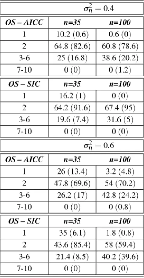
η were fixed, respectively, at 100 and 30 to obtain a SNR close to 4.5. The Tables 2 and 3 de-scribe the model order selection results for the temporal and spatial cases. As it can be seen from Table 2, AICC is most successful at small n, whereas SIC is most successful at large n. However, even if the highest frequencies are ob-served in correspondence of the correct model order, the difficulty of selecting the true order as the SNR decreases is evident. As regards the spatial context, the consistent property of the SIC statistic, that seems to pick the exact model
ση2=0:4
OS – AICC n=35 n=100
1 10.2(0.6) 0.6(0)
2 64.8(82.6) 60.8(78.6)
3-6 25(16.8) 38.6(20.2)
7-10 0(0) 0(1.2)
OS – SIC n=35 n=100
1 16.2(1) 0(0)
2 64.2(91.6) 67.4(95)
3-6 19.6(7.4) 31.6(5)
7-10 0(0) 0(0)
σ2
η=0:6
OS – AICC n=35 n=100
1 26(13.4) 3.2(4.8)
2 47.8(69.6) 54(70.2)
3-6 26.2(17) 42.8(24.2)
7-10 0(0) 0(0.8)
OS – SIC n=35 n=100
1 35(6.1) 1.8(0.8)
2 43.6(85.4) 58(59.4)
3-6 21.4(8.5) 40.2(39.6)
7-10 0(0) 0(0)
Table 2.The percentage of the order selected(OS)by
AICC and SIC criteria in 500 realizations of the AR(2)
process with measurement error variance equal to 0.4 and 0.6. In brackets are the percentage of the order
selected for the noise-free AR(2)process.
Selected
ISO-M FO-M SO-M
Simulated (2020)
ISO-M 70(88) 14.5(10) 15.5(2)
FO-M 36.5(37.5) 42(59.5) 21.5(3)
SO-M 5.5(1) 4(3) 90.5(96)
Simulated (3232)
ISO-M 81(93) 12.5(7) 6.5(0)
FO-M 9(3.5) 73.5(93) 17.5(3.5)
SO-M 0(0) 0(0) 100(100)
Simulated (128128)
ISO-M 91(95) 6.5(5) 2.5(0)
FO-M 0(1.5) 97.5(94) 2.5(4.5)
SO-M 0(0) 2(1.5) 98(98.5)
Table 3.The percentage of the order selected(OS)by
the SIC criterion in 200 realizations of the GMRF. In brackets are the percentage of the order selected for the
as the image size becomes larger is also evident. However, a point worth noting is that although an image of size (20 20) has 400
observa-tions, multidirectional dependence structure of the spatial data complicates the identification phase. In fact, for the first order GMRF, there are 30% and 58% of wrong model selections, for the isotropic and homogeneous case, respec-tively.
5. Conclusions
We conclude this paper with some considera-tions. In Section 2.3 we have proposed an esti-mator of autoregressive model parameters that can be used in the automatic model selection phase when the data are corrupted by a mea-surement error. Because of its consistency, it can be used when huge data sets are available. In fact, with respect to the minimization of the exactmaximum likelihood(EML)function the
ALSEestimator can be calculated quickly at the low computational cost of O(n) steps. In the
spatial and spatio-temporal context, Coli and Ippoliti 7] showed that under general
bound-ary conditions EML can be calculated at the computational cost ofO(n
2
)steps; however, for
images of dimensions (128 128) or larger,
the algorithm is computationally slow. Thus, the choice between EML and ALSE regards a trade-off between simplicity and efficiency. In all the simulations σ2
η was treated as fixed and known. However, several techniques may be considered to obtain very good estimates. For example, in the field of wavelets, theMAD estimator 8], gives robust estimates at the low
cost ofO(n)operations. Additional techniques
are also described in 15].
References
1] AKAIKE, H., A new look at the statistical model
identification,IEEE Trans. Automat. Control1974; 19, pp. 716–723.
2] AKAIKE, H., Time series analysis and control
through parametric models, in Findley, D. edition, Applied Time Series Analysis, Academic Press, New York, 1974.
3] BESAGJ., Efficiency of pseudolikelihood estimation
for simple Gaussian fields, Biometrika 1977; 64, pp. 616–618.
4] BHANSALI, R.J. Order selection for linear time
se-ries models: a review, in T. Subba Rao editor, Developments in Time Series Analysis, Chapman & Hall, 1993, pp. 50–66.
5] BOX, G.E.P.ANDJENKINS, G.M.,Time Series
Ana-lysis: Forecasting and Control, 2nd Edition, San Francisco, 1976.
6] CRESSIEN.A.C.,Statistics for Spatial Data, Wiley,
New York, 1993.
7] COLI, M.ANDIPPOLITI, L., Maximum Likelihood
Estimation of Noisy Gaussian Markov Random Fields, in Glavinic, V., Hljuz Dobric, V. and Simic, D. editors, Proceeding 24th International Confer-ence on Information Technology Interfaces ITI 2002; Cavtat, Croatia, June 24–27, 2002.
8] DONOHO D.L., JOHNSTONEI.M., Adapting to
un-known smoothness via wavelet shrinkage, JASA 1995; 90:1200–24.
9] DRYDENI., IPPOLITIL., ROMAGNOLIL., Adjusted
Maximum Likelihood and Pseudo-Likelihood Esti-mation for Noisy Gaussian Markov Random Fields, Journal of Computational and Graphical Statistics 2002; 11(2).
10] GRIFFITH, D.A.ANDLAGONA, F., On the quality of
likelihood-based estimators in spatial autoregressive models when data dependence structure is misspec-ified,Journal of Statistical Planning and Inference 1998, 69, pp. 153–174.
11] GUYON, X.ANDYAO, J.F., On the underfitting and
overfitting sets of models chosen by order crite-ria,Journal of Multivariate Analysis1999; 70, pp. 221–249.
12] HAMILTON, J.D., Time Series Analysis, Princeton
University Press, 1994.
13] HANNAN, E.J.ANDQUINN, B.G., The determination
of the order of an autoregression, J.R.S.S. 1979; B41, pp. 190–195.
14] HURVICH, C.M. AND TSAI, C.L., Regression and
time series model selection in small samples, Biometrika1989; 76, pp. 297–307.
15] IPPOLITI, L., ROMAGNOLI, L.ANDFONTANELLAL.,
A Noise Estimation Method for Corrupted Cor-related Data, Technical Report DMQTE 2/2003,
University of Pescara-Chieti.
16] JI, C.AND SEYMOUR, L., A consistent model
se-lection procedure for Markov random fields based on a penalized pseudolikelihood,Annals of Applied Probability1998; 6, pp. 423–443.
17] L ¨UTKEPOHL, H., Comparison of criteria for
estimat-ing the order of a vector autoregressive process, Journal of Time Series Analysis1985, 6, pp. 35–52.
18] NEWBOLD, P., Some recent developments in time
19] PARZEN, E., Some recent advances in time series
modelling and prediction problems, IEEE Trans. Auto. Control1974; AC-19.
20] SCHWARZ, G., Estimating the dimension of a model,
Ann. Statist., 1978, 8, pp. 461–464.
Received:June, 2003
Accepted:September, 2003
Contact address:
Mauro Coli, Lara Fontanella, Luigi Ippoliti Department of Quantitative Method and Economic Theory University “G. d’Annunzio”, Chieti Viale Pindaro 42 65127 Pescara, Italy e-mail:[email protected] [email protected] [email protected]
MAUROCOLIis professor of statistics at the Department of Quantitative Methods and Economic Theory, University G. d’Annunzio(Chieti),
where he is currently the coordinator of the Ph.D. courses in statistics. His main research interest includes spatial and spatio-temporal statis-tics with applications on social economic and environmental problems. He is a referee for the following journals: Statistica, Journal of Italian Statistical Society, Statistica Applicata; Ricerca Operativa.
LARAFONTANELLAreceived the Ph.D degree in statistics from the Uni-versity G. d’Annunzio of Chieti in 2001 and a postdoctoral research fellowship from 2001 to 2002. She is a member of the Department of Quantitative Methods and Economic Theory where she is currently a teaching and research assistant. Her research interests are in spatial and spatio-temporal geostatistical models with particular consideration to environmental phenomena.