Vol. 4, No. 4, 2011, 455-466
ISSN 1307-5543 – www.ejpam.com
Estimation and Selection in Regression Clustering
Guoqi Qian
1,∗, Yuehua Wu
21Department of Mathematics and Statistics, University of Melbourne, Melbourne, Australia
2Department of Mathematics and Statistics, York University, Toronto, Canada
Abstract. Regression clustering is an important model-based clustering tool having applications in a variety of disciplines. It discovers and reconstructs the hidden structure for a data set which is a random sample from a population comprising a fixed, but unknown, number of sub-populations, each of which is characterized by a class-specific regression hyperplane. An essential objective, as well as a preliminary step, in most clustering techniques including regression clustering, is to determine the underlying number of clusters in the data. In this paper, we briefly review regression clustering methods and discuss how to determine the underlying number of clusters by using model selection techniques, in particular, the information-based technique. A computing algorithm is developed for estimating the number of clusters and other parameters in regression clustering. Simulation studies are also provided to show the performance of the algorithm.
2000 Mathematics Subject Classifications: 62H30, 68T10, 91C20
Key Words and Phrases: Regression clustering, Least squares estimation, Model selection
1. Introduction
Cluster analysis is an important scientific tool for examining multivariate data with a view to uncovering or discovering clusters or groups of homogeneous observations. It finds clusters in the data such that observations are as “similar” as possible within clusters (internal cohe-sion or homogeneity), and as “dissimilar” as it could be between clusters (external separation or heterogeneity). Cluster analysis should be distinguished from the related problem of dis-criminant analysis in that it actually establishes the clusters, whereas in disdis-criminant analysis, known clusterings (or groupings) of some observations are used to categorize others and infer the structure of the data as a whole.
Clustering techniques range from those that are largely heuristic and descriptive to more formal procedures based on statistical models. In general, they follow either a hierarchical strategy or partitioning type of methods. Hierarchical methods proceed by stages producing a series of partitions, which may run from a single cluster containing all objects to as many
∗Corresponding author.
Email addresses:g.qianms.unimelb.edu.au(G. Qian),wuyhmathstat.yorku.a(Y. Wu)
clusters as the total number of objects, with each containing a single object. They can be either “agglomerative”, meaning that groups are merged, or “divisive”, in which one or more groups are split at each stage.
At each stage of hierarchical clustering, the splitting or merging is chosen so as to optimize some criterion. Conventional agglomerative hierarchical methods use heuristic criteria, such as single linkage (nearest neighbor), complete linkage (furthest neighbor), centroid cluster-ing, or sum of squares etc. [11]. In applications, divisive methods are less commonly used than agglomerative procedures since they are computationally demanding.
Yet a significant drawback of hierarchical clustering methods is that the divisions or fu-sions, once made, are irrevocable. When an agglomerative algorithm has joined two objects into a cluster they cannot subsequently be separated, and when a divisive algorithm has made a split, the objects cannot be recombined. As Kaufman and Rousseeuw[11]comment: “A hi-erarchical method suffers from the defect that it can never repair what was done in previous steps”.
In contrast, a partitioning method constructs a fixed number of clusters, sayk. It classifies the data intokclusters, which together satisfy two requirements of a partition: (i) each cluster must contain at least one object; (ii) each object must belong to exactly one cluster. Usually, partitioning methods move observations iteratively from one cluster to another, starting from an initial partition, to achieve some pre-chosen optimization. In most circumstances, the number of clusters has to be specified in advance and typically does not change during the course of the iteration. For instance, the most commonly used relocation methods – the
k-means type of methods: k-means, k-modes, k-medians and k-mediods [9, 10] – reduce the average within-group distance of objects to their nearest representatives (means, modes, medians or medoids).
We can easily envision that to identify possible clusters of observations in data, it is of essential importance to have the knowledge of how “close” individuals are to each other, or how far apart they are. The aforementioned methods such as the single linkage, complete linkage, k-means, etc. are usually considered as descriptive methods since they are mainly heuristically motivated and use descriptive statistics as the measures of similarity or dissimi-larity between observations. For instance, the k-means type of methods are characterized by taking the distance (Euclidean or Manhattan or Minkowski distances) of each object to the cluster centres (mean, median, mode, medoid) as the similarity or dissimilarity measure. On the other hand, model-based clustering uses a probability model as the similarity or dissimi-larity measure, i.e. objects have the same model specification within clusters. Furthermore, model-based clustering techniques use inferential statistics by means of probabilistic mod-els, not only for checking the significance of clusters and clustering, but also for providing a firm theoretical basis for clustering methods and strategies. Model-based methods can be applied both in hierarchical clustering and partitioning-type clustering. This research focuses on partitioning-type model-based approaches.
the mathematical relationship between high-density clusters and the single-linkage clustering method.
Consider a finite set of n objects O = {1, . . . ,n} together with data y1, . . . ,yn ∈Rp de-scribing the properties of these objects. Based on these data, our problem is to recover the latent partitioning Π = (C1, . . . ,Ck) ofO and to construct a clustering of the corresponding objects. A model-based or probabilistic clustering approach assumes that the observed data y1, . . . ,yn are a sample of random vectorsY1, . . . ,Yn that belong to a structured population.
It characterizes the clusters by specifications for the probability distribution of the random vectorsY1, . . . ,Yn which may differ from cluster to cluster.
Roughly speaking, stochastic model-based clustering techniques can be divided into the following two categories: (1) Parametric approach in which the probability distribution of Y1, . . . ,Yn is assumed to have a known parametric form but with unknown parameters; (2)
Non-parametric approach in which no distributional assumption is explicitly made for the individual clusters.
This paper will focus on parametric model-based partitioning-type clustering methods, in particular, the likelihood method. Further, we study only the regression clustering problem, which means the data y1, . . . ,yn contain observations of both dependent and explanatory variables and their relationship is of our interest. In Section 2, we review regression clustering. In Section 3, we discuss a procedures for estimating the parameters and the number of clusters in linear regression clustering under the classification likelihood framework. In Section 4, an algorithm is given for selecting the clustering and the number of clusters in regression clustering. The simulation study is presented in Section 5. Finally, Section 6 provides some discussions and concludes the paper.
2. Regression Clustering
Regression clustering refers to estimating the class-specific regression hyperplanes under-lying the data that randomly come from a population consisting of distinct classes. Note that the notion hyperplane used here is a generic one, which means it does not necessarily pass through the origin in the space. It should be more correctly called an affine set. But we do not distinguish them in this paper.
For the regression clustering problem, the data have the form(yj,x′j),j=1, . . . ,n, where xj ∈Rp is a (non-random) explanatory column vector and yj ∈Ra random dependent
vari-able for the j-th object. As in the general setting of model-based clustering, there are also two different approaches for regression clustering in the literature. One is the random partition re-gression clustering. The discussion can be found in[16, 15]among others. Another one is the fixed partition regression clustering. As discussed in[4, 5, 6, 7], the classification likelihood model or the fixed partition regression clustering model for any partitionΠ = (C1, . . . ,Ck)of O is:
Yj∼ f(·;βi,σi)∼φ(x′jβi,σi)for all j∈ Ci, i=1, . . . ,k.
Equivalently, it can be written in the form of a group of linear models:
Under the fixed-partition model (1), the log-likelihood function is given by
logLn(k,(βi,σ2i)i=1,...,k) =−
1 2
k
X
i=1
X
j∈Ci
log 2π+logσ2i +(yj−β
′
ixj)2
σ2i
. (2)
For given( ˆβi,σˆ2i)i=1,...,k, (2) is maximized at settingCi to
ˆ
Ci=arg min
i logσˆ
2
i +
(yj−βˆ′ixj)2
ˆ σ2i
!
. (3)
For given Cˆi, (2) is the sum of the usual log-likelihood functions for homogeneous linear
regressions within clusters. Hence, it is maximized by the LS-estimator βˆi from the data points(yj,xj)with j∈ Ci and
ˆ σ2i =
P
j∈Cˆi(yj−
ˆ β′ixj)2
ˆ
ni , i=1, . . . ,k, (4)
where nˆi =|Cˆi| is the number of data points inCi. Then logˆLn is monotonically increased if the steps (3) and (4) are carried out alternately. This algorithm leads to a local maximum (one would hope, to an approximation of the global maximum by proper initialization) in finitely many steps.
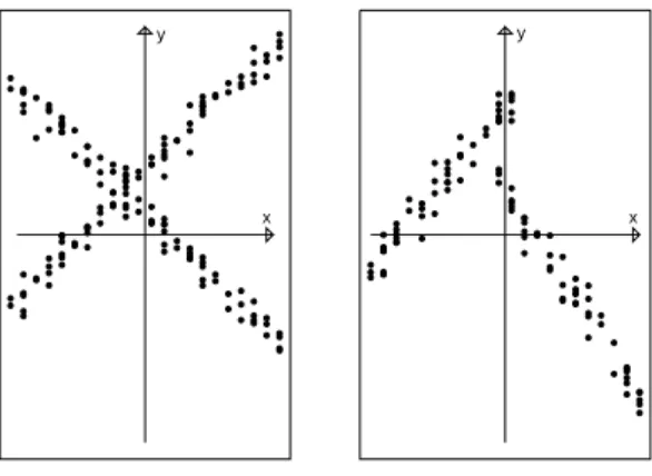
The fixed partition approach has a particular advantage over the random partitioning in the context of regression clustering. As observed by Hennig[1], the mixture model presumes implicitly anassignment independenceof each object to clusters with respect to the covariate vectorsxj. That is, the clusters keep the same conditional proportionsπi,i=1, . . . ,kfor every
fixed covariate vectorxj. In other words, the probability of a point(yj,x′j)to be generated by
clusteriis independent ofx and j. This is generally not true as shown in Figure 1, which is adapted from[1]. On the other hand, the fixed partition model (1) supposes that the cluster membership of each object or cluster labels are explicitly parametrized and are determined by the estimation ofβbi andσˆ2i through the points(yj,x′j)(j∈ Ci). Hence the fixed partition model does make allowance of possibleassignment dependencebetween the j-th object and the associated covariatexj.
3. Procedures for Estimating the Parameters and the Number of Clusters in
Regression Clustering
Suppose that we havenobjectsO(n)={1, 2, . . . ,n}with the associated data points
(x1,y1), . . .,(xn,yn). Here xj ∈Rp is a non-random explanatory p-vector and yj ∈R is a
x y
x y
Figure 1: Assignment independence – assignment dependence
this population, there exists an underlying partitionΠ(k0n)={O1(n), . . . ,Ok0(n)}, and each cluster
O(n)
i ¬{i1, . . . ,ini} ⊆ O
(n)is represented by
yO
i =XOiβ0i+eOi, eOi ∼N(0,σ 2
iIni), (5)
whereyO
i = (yi1, . . . ,yini) ′,X
Oi = (xi1, . . . ,xini)
′is ann
i×pdesign matrix in the clusterOi,eOi is anni-vector of random errors,Ini is anni×niidentity matrix, andni=|Oi|fori=1, . . . ,k0. Here,(β′0i,σi)′∈Rp×R+, 1≤i≤k0, arek0unknown parameter vectors.β0i, 1≤i≤k0, are
assumed to be distinct from one another. It is clear thatn=n1+. . .+nk
0. In the following, we
assume thatk0≤K, whereKis a known positive integer. Note that in (5) we have suppressed
theninOi(n)for convenience.
The objective is to reconstruct the underlying structure (5) from the observed data by estimating the number of clustersk0 and then classifying the data and estimating the
class-specific parameters accordingly. What can be done in practice, however, is to first consider every given partition of these n observations: Π(kn) = {C1(n), . . . ,Ck(n)}, where k ≤ K is a positive integer. For such a partition, one then fitskclusterwise regression models and obtain
kLeast Squares (LS) estimatesβbi,i=1, . . . ,k. By this stage, one can use a criterion to select the best k and the associated partition. Shao and Wu [14] propose an information-based criterion for determining the number of clusters as following: Letq(k)be a strictly increasing positive function ofk, andAn be a sequence of positive constants. Define
Dn(Π(kn)) =
k
X
i=1 ||yC(n)
i
−XC(n)
i
ˆ
βi||2+q(k)An, (6)
andˆkn, the estimate ofk0, is the integer that minimizes this criterion, i.e.
Dn(ˆkn) = min
1≤k≤KminΠ(n)
k
Dn(Π
(n)
where 1≤k≤K. It can be seen that in (6), the first term is the residual sum of squares which measures the goodness of fit of the model and the second term is the penalty for over-fitting. Furthermore, the criterion (7) shows that one determines the optimal number of clusters and the corresponding partitioning simultaneously. We shall call (7) Criterion LS-C in the sequel, which stands for clustering by the LS method.
Under some mild conditions, it is shown in Shao and Wu [14] that the proposed crite-rion selects the true number of regression hyperplanes with probability one among all class-growing sequences of classifications, when the number of observationsnfrom the population increases to infinity.
Note that the assumption eOi ∼ N(0,σ 2
iIni) in (5) is not required in computing the LS-estimatesβbi and the criterion function Dn(Π
(n)
k ). But the least squares estimates are known
to be sensitive to outliers and violation of the normality assumption in the data. This implies that the LS-C criterion is expected to work well for selecting the number of clusters and estimating the partition in linear regression clustering only when the normality assumption is not seriously violated. Recently, a consistent robust procedure for determining the number of clusters in regression clustering is proposed in[2]. However, we will not get into its theoretic detail here to keep this paper into reasonable length. We will use only the simulation in section 5 to illustrate the sensitivity of the LS-C criterion against normality.
Finally, it seems that each squared residual sum in the first term of (6) should be scaled by the corresponding variance estimateσˆ2i. Actually ignoring this scaling does not affect the asymptotic properties of the criterion functionDn(Π
(n)
k ). It turns out that ignoring the scaling
would improve the robustness of the clustering procedure. This is because a largeσ2
i estimate
is more likely to be associated with a cluster with large variability, thus being less separable from the other clusters. Ignoring the scaling would favor not including the outlaying data points in the current cluster.
4. An Algorithm for Estimation and Selection in Regression Clustering
We give an iterative algorithm in this section to implement the procedures in the previous section for selecting the optimal clustering and estimating the number of clusters in regression clustering.
For each fixed k, we obtain the optimal clustering of the dataΠk={C1, . . . ,Ck}by
mini-mizing the within-cluster sum of residual squares. The quantity to be minimized is then
SRSS(Πk) =
k
X
i=1
||yCi −XC′
iβbi||
2 (8)
where βbi, i = 1,· · ·,k, are the least squares estimators based on given {C1, . . . ,Ck}. This
minimization can be accomplished according to the following algorithm:
(i) Label all the data points in the sample as 1 ton. Given an initial partition
(ii) Seti=i+1 and reseti=1 ifi>n. Supposei∈ Cj. Then moveiintoCh,h=1, . . . ,k,
h6= j respectively. For each of these k−1 relocations, re-fit the regression models for the changed clusters and calculate the overall sum of the squared residuals accordingly. Denote the smallest one by SRSSh. If SRSSh<SRSS0, redefine
Cj=Cj− {i},Ch=Ch+{i}, and set SRSS0=SRSSh. Otherwise keepiinCj.
(iii) Repeat (ii) until the objective function (8) could not be reduced any further, which means no observation relocation is necessary and the optimal clustering is achieved for thisk.
The idea behind the above algorithm comes from[7]. Once the optimal clustering is done for each possiblek, the Criterion LS-C is used as a rule to select the best number of clusters.
It is noted that the initial partition of O = {1, . . . ,n}, if properly set, will facilitate the convergence and performance of the algorithm above. Denote the complement set of a setC
byCc. We propose to generate an initial partition of a dataset as follows:
Step 1. Consider the linear model
yi=x′iβ+ei. (9)
Based on the whole dataset, one estimates β by a robust method, e.g. least median squares method or least trimmed squares method[13].
Step 2. Put all data points, whose distances to the regression hyperplane estimated in Step 1 is less than a predetermined number, sayδ, into a setC1. If|C1| and|C1c|are both larger than a predetermined integer, saym, setℓ=1 and go to the next step; otherwise, set ℓ=0 and go to Step 5.
Step 3. Based on the datasetTℓi=1Cic, one estimatesβ in (9) by the same robust method used in Step 1.
Step 4. Put all data points inTℓi=1Cic, whose distances to the regression hyperplane estimated in Step 3 is less thanδ, into a setCℓ+1. If|Cℓ+1|and|Tℓi=+11Cic|are both larger thanm, setℓ=ℓ+1 and repeat Step 3; otherwise, go to Step 5.
Step 5. The initial partition is {C1, . . . ,Cℓ,Tℓi=1Cic} if ℓ > 1 or just the whole dataset itself if ℓ=0.
5. Simulation study
In this section we assess the finite sample performance of Criterion LS-C together with the use of the algorithm in the previous section. Simulated data sets are to be used to perform regression clustering for the assessment.
While many types of data sets can be simulated, we consider only two factors in determin-ing the type: number of clusters (2 or 3), and error distributions (standard normalN(0, 1)or
There will be only one covariate involved in the regression in each cluster, and the covariate is generated fromN(0, 1). The parameters used for each case are given in Table 2. Then the fixed partition regression clustering model yji = x′jiβ0i +eji,j = 1, . . . ,ni, i = 1, . . . ,k0 is applied to generate the response values yji, where eji is a random number originating from
N(0, 1) or t(3), and the first element of xji is the constant 1 corresponding to the intercept term in the model.
Table 1: Shorthand notation for the four cases.
N1C2 Case 1, two regression lines Normal error T1C2 Case 2, two regression lines t(3)error N1C3 Case 3, three regression lines Normal error T1C3 Case 4, three regression lines t(3)error
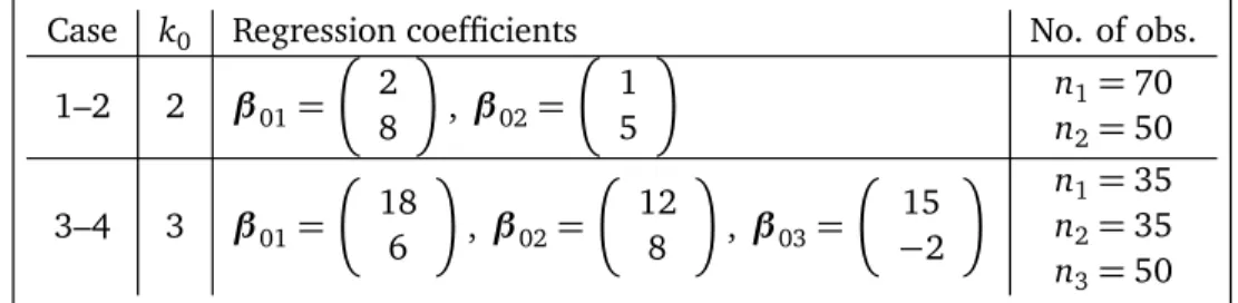
Table 2: Parameter values used in the simulation study of regression clustering.
Case k0 Regression coefficients No. of obs.
1–2 2 β01=
2 8
, β02=
1 5
n1=70
n2=50
3–4 3 β01=
18 6
, β02=
12 8
, β03=
15 −2
n1=35
n2=35
n3=50
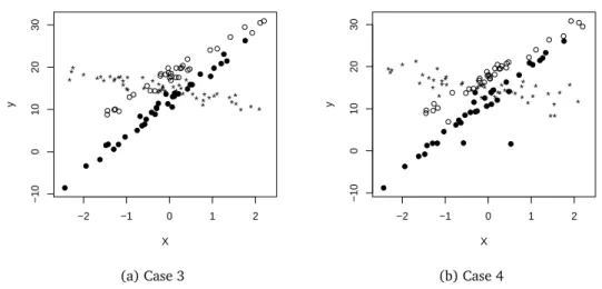
Figures 2 and 3 illustrate what the data typically would look like for Cases 1 to 4 with Normal ort(3)errors. These figures show that the groupings of the linear patterns are visible with standard normal random errors and getting worse witht(3)random errors.
−2 −1 0 1 2
−20
−10
0
10
20
X
y
(a) Case 1
−2 −1 0 1 2
−15
−5
0
5
10
15
20
X
y
(b) Case 2
−2 −1 0 1 2 −10 0 10 20 30 X y * * * * * ** ** * * * * * * * ** * * * * * * ** * * * * * * * * * * * * * * * * * * * * * * * *
(a) Case 3
−2 −1 0 1 2
−10 0 10 20 30 X y * * * * * * * * * * * * * * * * ** * * * * * * * * * * * * * * * * * * * * * * * * * * * * * * * *
(b) Case 4
Figure 3: Simulated data with three clusters.
In this study, we setq(k) =kpin Criterion LS-C (6), where pis the number of regression coefficients in the model and is a constant in our study; andkis the number of clusters used in the regression clustering under assessment. It is noted that in an information model selection criterion, a penalty function, which is An in (6), is usually chosen as clog(n) or clog log(n)
with a constant c > 0. In light of the fact that limλ→0
(logn)λ−1/λ= log logn, we set
An=(logn)3−1/3.
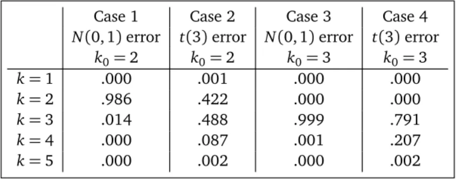
For each of the four cases, we conduct 1000 simulations using Criteria LS-C. To apply the algorithm given in Section 4, we set δ = 0.2 and m = 2p. The algorithm is then used to estimate the number of clusters in linear regression clustering. In Table 3 we summarize the results from the simulation study, where each number represents the relative frequency of selecting a given numberkclusters in regression clustering out of the 1000 replications.
From Table 3 we see that Criterion LS-C performs almost perfectly in Cases 1 and 3, which is expected since the errors are standard normal distributed. However, the criterion tends to over-estimate the number of clusters when the error distribution becomes heavy-tailed, as shown in Cases 2 and 4. This is also expected but it indicates that the direction of non-robustness of LS-C against normality is more likely to be over-clustering rather than under-clustering.
The cluster-specific regression lines can also be estimated during applying the criterion LS-C. Table 4 presents the estimation of the regression parameters by applying LS-C to the data shown in Figures 2 and 3. From the table, one can conclude that when the errors are
Table 3: Relative frequencies of selectingkbased on 1000 simulations for Cases 1-4.
Case 1 Case 2 Case 3 Case 4
N(0, 1)error t(3)error N(0, 1)error t(3)error
k0=2 k0=2 k0=3 k0=3
k=1 .000 .001 .000 .000
k=2 .986 .422 .000 .000
k=3 .014 .488 .999 .791
k=4 .000 .087 .001 .207
k=5 .000 .002 .000 .002
Table 4: The estimation of the regression parameters by applying LS-C to the data shown in Figures 2 and 3
k0 Case Clusters β1 β2 β3 β4
2 True
2 8
1 5
1 LS-C
2.12 8.02
0.76 5.11
2 LS-C
1.48 5.56
−1.13 5.87
4.46 6.18
3 True
18
6
12 8
15 −2
3 LS-C
18.05
6.06
11.97 8.02
14.66 −1.85
4 LS-C
17.74
6.14
12.02 8.16
10.73 −2.87
15.54 −1.70
6. Discussion
In this paper we review the general cluster analysis methods, then focus on regression clustering which uses the model-based fixed partition method and also takes into account the dependence between the response and explanatory variables. Regression clustering has not been widely used in practice even though it has a great potential. A possible reason is the computing complexity involved in the method. This paper provides a computing procedure and a feasible algorithm for estimation and selection involved in regression clustering. The simulation study concludes a satisfactory finite sample performance of the algorithm when the error distribution involved is close to normal. It also suggests the need to use a robust clustering method when the error distribution strays away from the normal.
References
[1] C Hennig. Identifiability of models for clusterwise linear regression. Journal of Classifi-cation, 17:273–296, 2000.
[2] C Rao and Y Wu and Q Shao. An M-Estimation-Based Procedure for Determining the Number of Regression Models in Regression Clustering. Journal of Applied Mathematics and Decision Sciences, 2007, 2007.
[3] D Pollard. Strong consistency ofk-means clustering.The Annals of Statistics, 9:135–140, 1981.
[4] H Bock. The equivalence of two extremal problems and its application to the iterative classification of multivariate data. Manuscript for the medizinische statistik conference, Forschungsinstitut Oberworfachl, 1969.
[5] H Bock. Probability models and hypotheses testing in partitioning cluster analysis. In P Arabie and L Hubert and G De Soete, editor,Clustering and Classification., pages 377– 453, River Edge, New Jersey., 1996. World Scientific Publishing.
[6] H Späth. Clusterwise linear regression.Computing, 22:367–373, 1979.
[7] H Späth. Algorithm 48: A fast algorithm for clusterwise linear regression. Computing, 29:175–181, 1982.
[8] J Hartigan. Consistency of single linkage for high-density clusters. Journal of the Amer-ican Statistical Association, 76:388–394, 1981.
[9] J Hartigan and M Wong. Algorithm as 136: Ak-means clustering algorithm. Applied Statistics, 28:100–108, 1978.
[11] L Kaufman and P Rousseeuw. Finding Groups in Data. Wiley-Interscience, New York, 1990.
[12] M Wong. A hybrid clustering method for identifying high-density clusters. Journal of the American Statistical Association, 77:841–847, 1982.
[13] P Rousseeuw and A Leroy. Robust Regression and Outlier Detection. Wiley, New York, 1987.
[14] Q Shao and Y Wu. A consistent procedure for determining the number of clusters in regression clustering. Journal of Statistical Planning and Inference, 135:461–476, 2005.
[15] R Quandt and J Ramsey. Estimating mixtures of normal distributions and switching regressions.Journal of the American statistical Association., 73:730–752, 1978.