https://doi.org/10.5194/os-15-601-2019
© Author(s) 2019. This work is distributed under the Creative Commons Attribution 4.0 License.
Numerical issues of the Total Exchange Flow (TEF) analysis
framework for quantifying estuarine circulation
Marvin Lorenz1, Knut Klingbeil1, Parker MacCready2, and Hans Burchard1
1Leibniz Institute for Baltic Sea Research Warnemünde, Physical Oceanography and Instumentation, Rostock, Germany 2University of Washington, College of Environment, School of Oceanography, Seattle, WA, USA
Correspondence:Marvin Lorenz ([email protected]) Received: 18 December 2018 – Discussion started: 4 February 2019 Revised: 23 April 2019 – Accepted: 6 May 2019 – Published: 29 May 2019
Abstract.For more than a century, estuarine exchange flow has been quantified by means of the Knudsen relations which connect bulk quantities such as inflow and outflow volume fluxes and salinities. These relations are closely linked to es-tuarine mixing. The recently developed Total Exchange Flow (TEF) analysis framework, which uses salinity coordinates to calculate these bulk quantities, allows an exact formulation of the Knudsen relations in realistic cases. There are how-ever numerical issues, since the original method does not converge to the TEF bulk values for an increasing number of salinity classes. In the present study, this problem is in-vestigated and the method of dividing salinities, described by MacCready et al. (2018), is mathematically introduced. A challenging yet compact analytical scenario for a well-mixed estuarine exchange flow is investigated for both meth-ods, showing the proper convergence of the dividing salinity method. Furthermore, the dividing salinity method is applied to model results of the Baltic Sea to demonstrate the analy-sis of realistic exchange flows and exchange flows with more than two layers.
1 Introduction
The Total Exchange Flow (TEF) analysis framework calcu-lates time-averaged net volume and mass transport between enclosed volumes of the ocean and ambient water masses, sorted by salinity classes. Since oscillatory inflow and out-flow components occurring at the same salinity compensate for one another, TEF characterises the net exchange flow with the ambient ocean. Salinity rather than density or tem-perature is used as a coordinate for calculating estuarine
ex-change flow, since only the salt budget is entirely controlled by the exchange flow. Therefore, salt is the only conserved quantity. In contrast, temperature and thus density are addi-tionally affected by the freshwater runoff and the surface heat fluxes.
A first bulk approach based on inflow and outflow salin-ity and volume transport had been developed and applied to the exchange flow of the Baltic Sea by Knudsen (1900). The theoretical framework based on a continuous salinity space was first developed by Walin (1977) and was later applied to exchange flow in the Baltic Sea (Walin, 1981). A comparable framework had been applied by Döös and Webb (1994) for quantifying meridional overturning circulation in the South-ern Ocean. Both the bulk concept by Knudsen (1900) and the continuous concept by Walin (1977) had been consistently combined by MacCready (2011), who also coined the term TEF.
The TEF analysis framework considers a time-averaged transport of a tracerc,Qc, through the cross-sectional area
A(s > S), which has a salinitysabove a specific valueS.Qc
is defined as
Qc(S)= *
Z
A(s>S) c udA
+
, (1)
whereuis the incoming velocity normal toA(s > S)with the definition that positiveubrings water into the estuary andh i denotes temporal averaging. The exchange profile of tracer flux per salinity as a function of the salinity is then obtained by differentiatingQc(S)with respect toS:
qc(S)= −∂Q
c(S)
such that Qc can be also obtained via integration ofqc in salinity space:
Qc(S)= Z
S0>S
qc(S0)dS0=
Smax Z
S
qc(S0)dS0. (3)
Based on these quantities, consistent Knudsen bulk values for inflowing and outflowing salinity (sin,sout), volume flux (Q1in=Qin,Qout) and salt flux (Qsin,Qsout), obeying
sin=
Qsin Qin
, sout=
Qsout Qout
, (4)
can be obtained. MacCready (2011) calculates the inflowing and outflowing bulk fluxes by integrating over positive and negative parts ofqc:
Qc,insign=
Smax Z
Smin
(qc)+dS, Qc,outsign=
Smax Z
Smin
(qc)−dS, (5)
where, for any function a, the positive part is calculated as (a)+=max(a,0)and the negative part is calculated as
(a)−=min(a,0). In (5),SminandSmaxare the minimum and maximum salinities. We will call this method of integrating positive and negative contributions separately to obtain the
QcinandQcoutsign method in the following.
Recently, Klingbeil et al. (2019) showed the relation be-tween TEF and thickness-weighted averaging. The concepts by Knudsen (1900), Walin (1977) and MacCready (2011) were focused on estuarine systems, which are characterised by distinct volume inflow Qr of water masses of (almost) zero salinity. The exchange flow between the estuary and the ocean is described by the Knudsen bulk values. The TEF analysis framework provides one consistent calculation method for these bulk values, which for this case describe the net exchange flow. Since there is no clear definition of the Knudsen bulk values, we will call these “TEF bulk val-ues” to distinguish between other bulk values which also ful-fill the Knudsen relations, e.g. bulk values computed from a Eulerian version of TEF. The Knudsen relations have been reviewed in detail for exchange flow in the western Baltic Sea by Burchard et al. (2018). Recently, MacCready et al. (2018) showed how the bulk concept can be used to esti-mate the volume-integrated average mixing M (defined as the rate of reduction of the net salinity variance due to mix-ing) in estuaries:M≈sinsoutQr, i.e. the volume-integrated average mixing in an estuary is approximated by the product of inflow and outflow salinity with the estuarine freshwater supply. This mixing estimate by MacCready et al. (2018) ap-proximates the TEF-based exact formulations developed by Burchard et al. (2018b).
Since the TEF analysis framework is continuous in salin-ity, a discretisation in salinity space is required when
analysing data from numerical model simulations or field ob-servations. In their Appendix A2, Klingbeil et al. (2019) pre-sented the remapping of discrete data into bins. As a result, the output of a numerical model consists of a finite number of transport values associated with the same number of dis-crete salinities. Comparable to a histogram, the transport data are binned into salinity classes according to their associated salinities. As discussed by MacCready et al. (2018), the re-sulting TEF profiles can become noisy, i.e. the sign changes inqc, when the number of discrete salinity classesN is cho-sen too high. For data sets with pairwise disjunct salinities, the number of transport values assigned to a single salinity bin decreases with the number of the salinity bins. After ex-ceeding a threshold number of salinity classes, the bins will be sufficiently small to hold at most one transport value. In this case,Qsignin is equal toQabsin , with
Qabsin = *
Z
A u+dA
+
. (6)
In most practical applications, the salinity data are neither constant in space nor time, and in the limit of an infinite num-ber of salinity classesQsignin will converge toQabsin , which is not the desired result forQin.
In order to obtain robust bulk values, which are less sensi-tive to the number of salinity bins, MacCready et al. (2018) suggested an alternative to the sign method. Instead of find-ing an optimal number of bins (a problem well known for histograms; Knuth, 2006), they suggested to find a divid-ing salinitySdiv which separates the inflow and outflow of a classical two-layer estuary with inflow at high and out-flow at low salinity classes, i.e.qc(Sdiv)=0 andQc(Sdiv)= max(Qc(S)). The bulk values for inflow and outflow are then obtained by integrating
Qc,indiv=
Smax Z
Sdiv
qcdS, Qc,outdiv=
Sdiv Z
Smin
qcdS. (7)
It should be noted that analytically, and for smoothqc with only one zero crossing, both methods coincide. We will show in Sect. 2 the different convergence behaviours and will show that the dividing salinity method indeed converges towards robust TEF bulk values, e.g. lim
N→∞Q div
in (N )=Qin, where
Qdivin denotes the inflowing volume flux computed with the dividing salinity method (7) forc=1.
nu-merical output from a model of the Baltic Sea, before we conclude in Sect. 5.
2 Convergence analysis for an analytical classical exchange flow
To demonstrate the different convergence behaviours of the sign method and the dividing salinity method, we take the analytical example from Burchard et al. (2019). It describes a well-mixed tidal flow with oscillating salinity as it occurs, e.g. in the Wadden Sea (Purkiani et al., 2015). The velocity and salinity are given by
u(t )=ur+uacos(ωt ), s(t )=sr+sacos(ωt+φ), (8) with the residual velocity ur<0, the residual salinity sr, the velocity and salinity amplitudesua>0 andsa>0, with
sr−sa≥0, the tidal frequencyω=2π/T with the tidal pe-riod T and the tidal phaseφ. The tidally averaged salinity transport is given by
1
T T Z
0
usdt=ursr+
uasa
2 cos(φ). (9)
Zero residual salt transport therefore requires cos(φ)= −2ursr
uasa
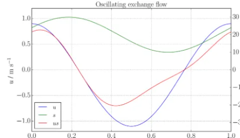
with uasa≥2|ur|sr. (10) Figure 1 shows an example for u(t ), s(t ) and u(t )·s(t ), with A=10 000 m2, ur= −0.1 m s−1, ua=1 m s−1, sr= 20 g kg−1 and s
a=10 g kg−1, resulting in φ= −1.16= −0.185·2π. In this case,Q(S),Qs(S)andSdivcan be calcu-lated analytically by either (5) or (7) (see Appendix A) and are shown in Fig. 2d. By means of (4), the inflow and out-flow volume fluxes and salinities,Qin,Qout,sinandsout, can then be exactly calculated. The resulting analytical TEF bulk values areQin=813.240 m3s−1,Qout= −1813.240 m3s−1,
sin=28.424 g kg−1andsout=12.748 g kg−1.
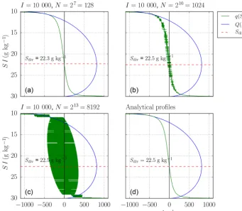
We created a time series ofI =105time steps of (8) and computedq(S)andqs(S)for a varying numberNof salinity classes betweenSmin=10 g kg−1andSmax=31 g kg−1; see Fig. 2. In Fig. 2a (N=128), the smallNleads to smooth pro-files for bothqandQ. Profiles of higher numbers (N=1024,
N =8192) of salinity classes exhibit more noisyqbut appar-ently still smoothQ(Fig. 2b, c). Comparison with the ana-lytical solution (Fig. 2d) shows thatQis similar for allNand
q becomes more noisy. This is a result of the numerical dis-cretisation of the data. Most likely, the numerical values (e.g. due to round-off errors) for these salinities are all different. Other than in continuous salinity space where inflows and outflows in the same salinity class partially compensate for one another, the corresponding discrete values could be as-sociated with different salinity classes and the compensation does not occur anymore, resulting in noisy profiles, which
Figure 1.Oscillating exchange flow (see Sect. 2): time series of velocity (blue), salinity (green) and salinity flux (red) for the oscil-lating exchange flow scenario (8).
leads to errors in the results of the sign method.Qonly ap-pears to be smooth, but the noise is of course apparent since
Qandqare dependent on each other. The integration process of the discreteqc(see (3)) smooths the resultingQc.
To study the convergence of the two different methods (the sign method and dividing salinity method), one can com-pare the errors in discrete form to the analytical values. Fig-ure 3 shows the relative error,|Qin(I, N )−Qin|/|Qin|, of the numerically computed inflow bulk values depending on the number of time stepsI and the number of salinity classes
Figure 2.Oscillating exchange flow (see Sect. 2): from (14) and (15) numerically(a–c)and analytically(d)foundQ(S)(blue),q(S)(green), dividing salinity,Sdiv(dashed, red), forI=104time steps for one tidal cycle and varying number of salinity classesN. With increasingN, qbecomes more noisy, whereasQseems unchanged.
Figure 3.Oscillating exchange flow (see Sect. 2): relative error ofQincomputed with(a)the dividing salinity method and(b)the sign
3 Extended dividing salinity method 3.1 Mathematical formulation
Encouraged by the good convergence behaviour of the di-viding salinity method demonstrated in the previous section, we introduce here a general formulation which includes in-verse estuaries and exchange flows with more than two lay-ers. The general idea is to identify the salinities which di-videqcinto inflowing and outflowing parts. This corresponds to zero crossings, dividingqc>0 andqc<0. Analytically, the zero crossings are calculated by solvingqc(Sdiv)=0 for
Sdiv. However, as the discreteqc might be very noisy with too many zero crossings (see Sect. 2), we propose finding the extrema of the discreteQcprofiles, which share the same salinities as the zero crossings. Figure 4 shows a hypothet-ical exchange flows of four layers, separated by five divid-ing salinities which can be sorted in ascenddivid-ing order:Smin=
Sdiv,1< Sdiv,2< Sdiv,3< Sdiv,4< Sdiv,5=Smax. The fluxes
1Qcj in each layer can be calculated by
1Qcj=
Sdiv, j+1 Z
Sdiv, j
qcdS=Qc(Sdiv, j+1)−Qc(Sdiv, j). (11)
In the next step, inflow segments with1Qcj>0 and outflow segments with1Qcj<0 can be identified and indexed. For the example in Fig. 4, we index starting fromSmin:Qcout,1=
1Qc1,Qcin,1=1Qc2,Qcout,2=1Qc3andQcin,2=1Qc4. The representative salinities are calculated for each inflow and outflow similar to (4):
sin, m= Qsin, m Qin, m
, sout, m= Qsout, m Qout, m
, (12)
wheremdenotes the index withm=1,2 and so on. For a classical estuary, (11) reads as (7), where the only dividing salinity exceptSminorSmaxisSdiv=S(max(Qc)).
The mixing relations of MacCready et al. (2018) and Bur-chard et al. (2019) require only one value each for the inflow properties and outflow properties, respectively. These can be obtained from a multi-layer transect by applying weighted averages, i.e. for the inflowing bulk values:
Qcin=X
m
Qcin, m, cin= P
mQcin, m P
mQin, m
= P
mcin, mQin, m P
mQin, m
, (13)
and accordingly forQcoutandcout. 3.2 Discrete formulation
The output from a numerical model along a transect across an estuary is assumed to consist of I time steps with 1≤i≤I and 1≤k≤K, which are spatial increments per each time step. The output should include collocated model
Figure 4.Sketch of hypothetical TEF profiles of a four-layered sys-tem with alternating inflows and outflows,Qcin, mandQcout, m. The respective inflows and outflows are divided by the zero crossings of
qc(S)(green), so-called dividing salinities,Sdiv, j (dashed, black),
which correspond to the minima and maxima ofQc(S)(blue).
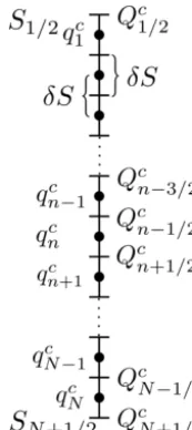
dataski (salinity),cik (tracer) and uik (incoming normal ve-locity) which are available on cross-sectional area incre-mentsAik. The salinity interval[S1/2, SN+1/2], withS1/2<
SminandSmax< SN+1/2, whereSmin=min(s)andSmax= max(s), is divided into N equidistant intervals of length
δS=(SN+1/2−S1/2)/N; compare Fig. 5. The discrete pro-files ofqc should be obtained directly without numerically calculating the volume flux profileQcbefore to avoid trun-cation errors due to numerical derivatives and to save com-putational time:
qnc= 1
I δS X
i X
k (forn=ni
k)
uikcikAik, with nik= $
ski−S1/2
δS !%
,
(14)
whereb·c is the integer truncation function. With this, the tracer flux increments are directly added to the respective salinity class; see the dots in the sketch of Fig. 5. Compu-tation ofQc(S) can be easily carried out by summation of
qnc:
Qcn−1/2=δS N X
n0=n
Figure 5.Sketch of howQcandqcare located in a discrete salin-ity space. The salinsalin-ity interval [S1/2, SN+1/2] is divided intoN
equidistant salinity classes of lengthδS. The entries ofQc(Qcn) are located on the lines, and the entries of qc (qnc) are located on the dots.
Using the extended dividing salinity method defined in (11), the calculation for the transport reads
1Qcj=Qcn=ndiv, j+1−Q c
n=ndiv, j, (16)
wherendiv, j andndiv, j+1 describe the indexes, where two consecutive extrema ofQc are located. The dividing salin-ity indices are calculated with an algorithm which searches
Q for local extrema by comparing every entry Qn+1/2 to its nearest neighbours (Qn−1/2 and Qn+3/2). If Qn+1/2 is greater (smaller) than its two neighbours,n+1/2 is stored as
ndiv, jand denoted maximum (minimum). Afterwards,
trans-port is computed according to (16), and only dividing salin-ities with transport greater than a threshold transportQthresh are considered. Please see Appendix B for a detailed descrip-tion.
4 Application to exchange flow in the Baltic Sea The Baltic Sea, shown in Fig. 6, can be considered as a large estuary with a long-term averaged river runoff of around 16 000 m3s−1and about balanced precipitation and evapora-tion (Matthäus and Schinke, 1999). In the estuarine classifi-cation diagram by Geyer and MacCready (2014), the Baltic Sea has been classified as a fjord type and a strongly strati-fied estuary, due to its relatively low runoff and relatively low mixing. The topography of the Baltic Sea consists of several basins of which the Gotland Basin in the central Baltic Sea, denoted as GB in Fig. 6, is the largest with a water depth of about 240 m. The shallow and narrow Danish Straits in the southwest provide the only connection to the saline North Sea.
Episodic inflow events of water consisting of a mixture of saline North Sea water and recirculated brackish Baltic Sea water (Meier et al., 2006) transport large amounts of salt and oxygen into the Baltic Sea. These inflows may either occur as major Baltic inflows (MBIs; i.e. as well-mixed, barotropic inflows) during winter months (Matthäus and Schinke, 1999; Mohrholz et al., 2015) or as baroclinic summer inflows (Feis-tel et al., 2004, 2006). These large inflow events propagate as dense bottom currents from basin to basin, where they are subject to entrainment of overlaying less saline water. The volume of the inflows increases and their salinity decreases on the way into the central Baltic Sea, where they ventilate the typically anoxic bottom layers (Reissmann et al., 2009). More frequent but weaker and less saline inflow events prop-agate through the western Baltic Sea (Sellschopp et al., 2006; Umlauf et al., 2007) and have the potential to ventilate in-termediate layers but not the bottom layers in the central Baltic Sea (Reissmann et al., 2009). The major mixing pro-cess to transport saline bottom waters towards the surface of the central Baltic Sea has been identified as boundary mix-ing (Holtermann et al., 2012, 2014). However, recently dou-ble diffusion in the stratified interior has been discussed as another possibly efficient mixing process in the Baltic Sea (Umlauf et al., 2018). Finally, various surface mixed layer processes mix the salt into the surface layer of the Baltic Sea, such that a horizontal surface salinity gradient is established, with salinities varying from 25 g kg−1 in the Kattegat (K) to 5 g kg−1in the Bothnian Bay (BoB). A permanent halo-cline separates these surface waters from the saline bottom waters. The halocline is located approximately in 70–90 m depth in the Gotland Basin. In addition, a seasonal thermo-cline develops during summer between 10 and 30 m (Reiss-mann et al., 2009). At times, salinity inversions occur in the strongly stratified thermocline, with surface waters being slightly more saline than waters in the thermocline (Burchard et al., 2017).
Above the halocline, driven by wind, inflows and Earth rotation, a cyclonic circulation is generally present in the central Baltic Sea, with net northward flow in the east of Gotland and southward flow in the west of Gotland (Meier, 2007; Omstedt et al., 2014). This cyclonic circulation is also present in the deeper layers of the central Baltic Sea, pos-sibly driven by inflows and boundary mixing processes (Ha-gen and Feistel, 2007; Meier, 2007; Holtermann and Umlauf, 2012). This deep-water mean circulation is overlaid by to-pographic waves and inertial oscillations (Holtermann et al., 2014).
Figure 6.Map and bathymetry of the Baltic Sea. K: Kattegat, D: Darss Sill and the Darss Sill transect (red), G: the Gotland island, GB: Gotland Basin and the Gotland transect (green), BoB: Bothnian Bay.
4.1 Exchange flow over Darss Sill
In their recent review paper, Burchard et al. (2018) applied the Knudsen relations and the TEF analysis framework to analyse 65 years of high-resolution numerical model output for the western Baltic Sea using the General Estuarine Trans-port Model (GETM) (Burchard and Bolding, 2002; Hofmeis-ter et al., 2010; Klingbeil and Burchard, 2013). Here, we in-vestigate numerical properties of the TEF calculations based on the same numerical model output for the complex inflow years (2002/2003) with several barotropic and baroclinic in-flows (Feistel et al., 2006) over the Darss Sill transect shown in Fig. 6.
The horizontal resolution of the model is about 600 m, and the water column is discretised by 42 vertical adaptive layers, the thickness of which vary in time and space (Gräwe et al., 2015). The salinity, velocity and layer thickness data are in-terpolated to 95 locations equally spaced by 1x=545 m along the 52 km long Darss Sill transect which is directed in northwest–southeast direction, such that the number of data points per time step is K=42·95=3990. The model out-put time step is1t=3 h, such thatI =5840 time steps for two simulation years are stored. These 3-hourly values are obtained by thickness-weighted averaging (Klingbeil et al., 2019) of the model layer values from all model time steps within the output interval.
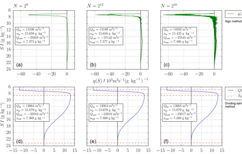
Application of the TEF analysis framework forN differ-ent salinity classes is shown in Fig. 7, where a classical two-layer exchange flow with inflow at high salinities is seen.
The upper panels showq and the respective TEF bulk val-ues, computed with the sign method.q becomes more noisy with increasingN. The bulk values still change with increas-ingN. The lower panels showQ for the sameN and the TEF bulk values computed with the extended dividing salin-ity method. These bulk values do converge for increasing
N towards constant values. For this case,Qthreshwas set to
Qthresh=100 m3s−1.
The values found in this study with the dividing salinity method confirm that the found bulk values in Burchard et al. (2018) are correct and did not experience great errors from using the sign method.
Similar to the dependency of the TEF bulk values onI in the oscillating exchange flow in Sect. 2, we investigate the dependency of the TEF bulk values on the temporal resolu-tion of the exchange flow. In order to do so, we repeated the TEF analyses for data obtained by thickness-weighted av-eraging of the 3-hourly model output to intervals of 12 h, and 1, 3, 5 and 10 d. For the dividing salinity method, the relative differences to estimated reference values for differ-ent time steps of the model output are calculated. The refer-ence bulk values have been calculated by the dividing salin-ity method forN=216=65 536 salinity classes and the 3-hourly output, since the exact values are not available. The hydrodynamic model was forced with 3-hourly atmospheric data, meaning that external processes of smaller timescales are not included. Therefore, the estimated bulk values can be considered as good estimations. Figure 8a showsQ(S, 1t )
with the corresponding dividing salinities. With coarser tem-poral resolution (larger1t), the maximum ofQmoves to-wards greater salinities and smaller transport values, show-ing a weakened exchange flow. For1t=10 d, the maximum shifts back to smaller salinities, indicating that some pro-cesses are not resolved anymore. Furthermore, the maximum salinities decrease with reduced temporal resolution, which indicates that the inflows of high salinities are not captured. In Fig. 8b, the relative deviations of the TEF bulk values are shown for the inflow. With increasing time step1t, the devia-tions increase rapidly as one would expect since processes of smaller timescales are not resolved anymore. For1t≥3 d, the deviations fluctuate around a constant value with the ex-ception of 1t=5 d. The deviations for this time step are smaller than expected. Figure 8a shows that the shape of
Figure 7.Exchange flow over Darss Sill: profiles ofq(a, b, c)andQ(d, e, f)for the Darss Sill transect in 2002/2003 depending on the number of salinity classesN:(a, d)N=28=256,(b, e)N=212=4096,(c, f)N=216=65 536. The respective TEF bulk values are calculated with the sign method (5) in panels(a, b, c)and the extended dividing salinity method (11, 16) in panels(d, e, f).
4.2 Cross section through the Gotland Basin
In this section, the capability of the extended dividing salin-ity method to be applied to exchange flows or transects with more than two layers is demonstrated. Here, example results are shown for model data of the Gotland Basin in the Baltic Sea. The analysed transect uses the model run from Burchard et al. (2018) consisting of 156 equally spaced locations with 1 nmi resolution and 50 vertical adaptive layers. Daily aver-ages from 2 simulation years, 2002 and 2003, are analysed. These 2 years show a complex inflow activity, with baroclinic inflows during summer 2002 and summer 2003 and an MBI during winter 2002/2003 (Feistel et al., 2006).
Figure 9a shows q for N=28=256 salinity classes to visualise the exchange flow, whereas Fig. 9b shows Qfor
N =216=65 536, which is used to compute the bulk values using the extended dividing salinity method (11 and 16). For this data set, five dividing salinities are found usingQthresh= 0.01·max(|Q|)≈700 m3s−1, separating two inflows (Qin,1 andQin,2) and two outflows (Qout,1andQout,2). These are listed with their respective salinities (sin,1,sin,2,sout,1and
sout,2) on the right of Fig. 9 forN=216salinity classes.
The net southward transport of 11 300 m3s−1results from the fact that most river input is entering the Baltic Sea north of the transect.Qin,1andQout,1belong to the cyclonic sur-face circulation of the Gotland Basin described above. With the main river input in the north, the outflowQout,1 is less saline than the inflowQin,1which experiences more entrain-ment of saline bottom waters during the recirculation.Qin,2 describes the net northward transport of the deep circula-tion which is fed with high salinities of the inflow events.
Figure 8.Exchange flow over Darss Sill: comparison ofQ(S)(N=216=65 536) for different1tin panel(a)and the relative deviations of
Qinandsinin dependency1tto the bulk values for1t=3 h in panel(b). The bulk values were computed fromQ(1t )using the extended
dividing salinity method (11, 16). The dashed lines in panel(a)show the dividing salinities used to compute the bulk values in panel(b). With different temporal resolutions, the shape ofQ(S)changes considerably and the resulting bulk values deviate significantly from the ones for 3-hourly data.
Figure 9.Cross section through Gotland Basin: profiles ofqforN=28=256(a)andQforN=216=65 536(b)for the Gotland transect in 2002/2003. Five dividing salinities separate two inflows and two outflows. The corresponding TEF bulk values are listed on the right.
5 Discussion and conclusions
This study investigated the numerical issues of the TEF anal-ysis framework, proposed by MacCready (2011). Two exist-ing calculation methods for the computation of the bulk val-ues of an exchange flow, the sign method (5) (MacCready, 2011) and the dividing salinity method (7) (MacCready et al., 2018), were compared in their respective convergence
con-vergent and robust calculation of TEF bulk values. An ex-tended formulation of the dividing salinity method is pre-sented which includes exchange flows of more than two lay-ers as well as invlay-erse exchange flows. We showed the appli-cation to two transects of the Baltic Sea. The main challenge of the extended dividing salinity method is finding the divid-ing salinities. We provide a detailed description of a robust algorithm to obtain extrema of Qwhich is required to de-termine the dividing salinities in Appendix B. Moreover, we investigated the dependency of the calculated bulk values on the frequency of model output. The results confirm that the output of the model for a transect which should be analysed by the application of TEF is strongly dependent on the phys-ical mechanism controlling the exchange flow.
Based on our results, we propose a best-practice procedure for calculating TEF from a numerical model:
1. At the level of setting up a numerical model, the spatial (horizontal and vertical) resolution should be chosen as high as possible to reproduce return flows due to lateral eddies and smaller overturns.
2. Once a transect for the TEF analysis has been identi-fied, the frequency for storing the output along that tran-sect has to be chosen. For analytical correctness, the binning of data of volume and salt fluxes into salinity classes should be done online within the hydrodynamic model at every model time step. Time-averaged model output of these binned data can directly be used for the TEF analysis. If the model only provides output within the model layers, the binning and averaging must be done offline during postprocessing. This would induce different kinds of errors: (i) instantaneous data snap-shots which skip intermediate model time steps do not conserve fluxes and do not consider intermediate salin-ity variations; (ii) model data obtained by thickness-weighted averaging over model time steps conserve fluxes but merge data of different salinities. Both types of errors can be reduced with a sufficiently high output frequency, such that the output data still resolve the dy-namics of the flow.
3. If the binning is not done online, required output fields are the velocity component normal to the transect, the salinity and the grid box area along the transect. We suggest that these variables are stored as thickness-weighted averaged values (Klingbeil et al., 2019) be-tween two output time steps to ensure the conservation of volume and salinity.
4. The results should be analysed for a large range of salin-ity classes N with the dividing salinity method (11) and (12) to check the convergence of the TEF bulk val-ues. In this study, N≈1000 salinity classes (∼δS= 0.02 g kg−1) were sufficient enough for all three inves-tigated examples with errors or deviations smaller than 0.1 %.
5. Visualisation of the exchange flow should still be done with a smoothq, since it shows the inflows and outflows more clearly. We suggest to chooseN≈250 for estuar-ies with a wide range of salinitestuar-ies or a step size in salin-ity space of∼0.05 g kg−1, i.e. 20 steps per 1 g kg−1, for estuaries with smaller salinity ranges.
Appendix A: Analytical solution forQ(S)andQs(S)
For the oscillating exchange flow given in (8), the analyti-cal solution is given here for the volume flux profile Q(S)
and the salinity flux profileQs(S). According to (1), these profiles are calculated as
Q(S)= *
Z
A(S) udA
+ =A
T t(2)(S)
Z
t(1)(S) u(t )dt
= A
ωT h
urωt+uasin(ωt ) it(2)(S)
t(1)(S), (A1)
and
Qs(S)= *
Z
A(S) usdA
+
=A
T t(2)(S)
Z
t(1)(S)
u(t )s(t )dt
= A
ωT
ursrωt+uasrsin(ωt )+ursasin(ωt+φ)
+uasacos(φ)
2 (ωt+sin(ωt )cos(ωt ))
−uasasin(φ)
2 sin
2(ωt )
t=t(2)(S)
t=t(1)(S)
, (A2)
with
t(1)(S)= −1
ω
arccos S−s
r sa +φ ,
t(2)(S)= 1
ω
arccos S−s
r sa −φ , (A3)
which ensures that s(t )≥S for t(1)(S)≤t≤t(2)(S) and
s(t ) < Sfort(2)(S) < t < t(1)(S)+T.q(S)is calculated ac-cording to (2):
q(S) = A
ωT q
s2
a−(S−sr)2 h
ut(1)+ut(2)i
= 2A
ωT q
s2
a−(S−sr)2
ur+ua
S−sr
sa
cos(φ)
.
(A4) The dividing salinity can be calculated by finding the root of
q(S). Solving (A4) withq(Sdiv)=0 forSdiv:
Sdiv= −saur
uacos(φ)
+sr. (A5)
The TEF bulk values can be calculated according to (7) and (4).
Appendix B: Algorithm description
The algorithm finding the extrema ofQworks as follows. First, every entryQn+1/2ofQis compared with its nearest neighboursQn−1/2andQn+3/2. IfQn+1/2is either the max-imum (minmax-imum) in this interval, the indexn+1/2 is stored and denoted by max (min), respectively. Afterwards, consec-utive maxima or minima are deleted, leaving only the great-est maxima or the smallgreat-est minima. Now, minima and max-ima should be alternating. At this stage, there are probably physically insignificant extrema found. Therefore, transport is calculated according to (16); their absolute values|1Qj| are compared to a given threshold valueQthresh, which we recommend to set to a value of 0.01·max(|Q|)m3s−1. If the transport |1Qj| is smaller than Qthresh,Q(Sdiv, j ) and Q(Sdiv, j+2)are compared and only the greater (smaller) of the two is kept to ensure that the greater maxima (smaller minima) remains. The two dividing salinities which belong to the smaller (greater) transport are then not considered any-more. If the first or last extremum is involved in this pro-cedure, only the extremum which is not the first or last ex-tremum is deleted. If this needs to be done, then the first or last extremum changes its property from either minimum to maximum or the other way round to ensure alternating min-ima and maxmin-ima. The last step is to adjust the first and last extrema to the index whereQn+1/2starts to differ fromQ1/2 (low salinities) or whereQn+1/2differs from 0 (high salin-ities). This step is not necessary for calculating the correct TEF bulk values since only the dividing part is important and not the exact value of the dividing salinity. Nevertheless, this procedure ensures thatSdiv,1 is the salinity class next to min(s)andSdiv, J+1is next to max(s), withJ being the number of layers.
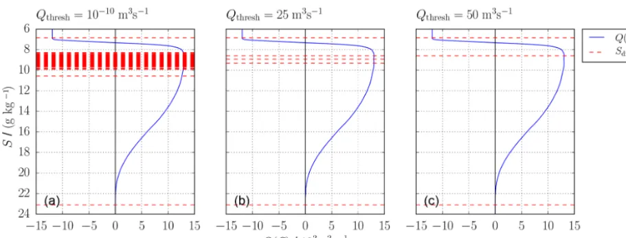
Figure B1 shows the sensitivity of the number of di-viding salinities on Qthresh for the data from Sect. 4.1 for N=4096 salinity classes. In Fig. B1a, for Qthresh= 10−10m3s−1 (to filter out numerical noise of double-precision data), 135 dividing salinities, most between 8 and 10 g kg−1, are found. Most of them are noise carried on from the q profile to Q and have no physical meaning. How-ever, two major transport values are found: −24 885 and 12 603 m3s−1. ForQthresh=25 m3s−1, noise-related trans-port values are filtered out, leaving two small transtrans-port val-ues of 63 and −44 m3s−1. The two main transport val-ues change to −25 016 and 13 045 m3s−1. Increasing to
the exact same results as Fig. 7b, whereQthresh=100 m3s−1 was used.
Figure B1.Comparison of the algorithm for(a)Qthresh=10−10m3s−1,(b)Qthresh=25 m3s−1and(c)Qthresh=50 m3s−1for the Darss
Competing interests. The authors declare that they have no conflict of interest.
Acknowledgements. This paper is a contribution to BMBF-GROCE FKZ 03F0778. Hans Burchard and Marvin Lorenz were supported by Research Training Group Baltic TRANSCOAST GRK 2000 funded by the German Research Foundation. Knut Klingbeil was supported by the Collaborative Research Centre TRR 181 on En-ergy Transfer in Atmosphere and Ocean funded by the German Re-search Foundation (project no. 274762653), and Parker MacCready was supported by US National Science Foundation (grant no. OCE-1736242).
Financial support. The publication of this article was funded by the Open Access Fund of the Leibniz Association.
Review statement. This paper was edited by Eric J. M. Delhez and reviewed by two anonymous referees.
References
Burchard, H. and Bolding, K.: GETM, A General Estuarine Trans-port Model: Scientific Documentation, Tech. Rep. EUR 20253 EN, Eur. Comm., 2002.
Burchard, H., Basdurak, N. B., Gräwe, U., Knoll, M., Mohrholz, V., and Müller, S.: Salinity inversions in the thermocline under upwelling favorable winds, Geophys. Res. Lett., 44, 1422–1428, 2017.
Burchard, H., Bolding, K., Feistel, R., Gräwe, U., Klingbeil, K., MacCready, P., Mohrholz, V., Umlauf, L., and van der Lee, E. M.: The Knudsen theorem and the Total Exchange Flow analysis framework applied to the Baltic Sea, Prog. Oceanogr., 165, 268– 286, https://doi.org/10.1016/j.pocean.2018.04.004, 2018. Burchard, H., Lange, X., Klingbeil, K., and MacCready, P.:
Mix-ing Estimates for Estuaries, J. Phys. Oceanogr., 49, 631–648, https://doi.org/10.1175/JPO-D-18-0147.1, 2019.
Döös, K. and Webb, D. J.: The Deacon cell and the other meridional cells of the Southern Ocean, J. Phys. Oceanogr., 24, 429–442, 1994.
Feistel, R., Nausch, G., Heene, T., Piechura, J., and Hagen, E.: Evi-dence for a warm water inflow into the Baltic Proper in summer 2003, Oceanologia, 46, 581–598, 2004.
Feistel, R., Nausch, G., and Hagen, E.: Unusual Baltic inflow activ-ity in 2002-2003 and varying deep-water properties, Oceanolo-gia, 48, 21–35, 2006.
Geyer, W. R. and MacCready, P.: The estuarine circulation, Annu. Rev. Fluid Mech., 46, 175–197, 2014.
Gräwe, U., Holtermann, P., Klingbeil, K., and Burchard, H.: Ad-vantages of vertically adaptive coordinates in numerical models of stratified shelf seas, Ocean Model., 92, 56–68, 2015. Hagen, E. and Feistel, R.: Synoptic changes in the deep rim current
during stagnant hydrographic conditions in the Eastern Gotland Basin, Baltic Sea, Oceanologia, 49, 185–208, 2007.
Hofmeister, R., Burchard, H., and Beckers, J.-M.: Non-uniform adaptive vertical grids for 3-D numerical ocean models, Ocean Model., 33, 70–86, 2010.
Holtermann, P. L. and Umlauf, L.: The Baltic Sea Tracer Release Experiment: 2. Mixing processes, J. Geophys. Res.-Oceans, 117, https://doi.org/10.1029/2011JC007445, 2012.
Holtermann, P. L., Umlauf, L., Tanhua, T., Schmale, O., Re-hder, G., and Waniek, J. J.: The Baltic Sea Tracer Release Experiment: 1. Mixing rates, J. Geophys. Res.-Oceans, 117, https://doi.org/10.1029/2011JC007439, 2012.
Holtermann, P. L., Burchard, H., Graewe, U., Klingbeil, K., and Umlauf, L.: Deep-water dynamics and boundary mixing in a non-tidal stratified basin: A modeling study of the Baltic Sea, J. Geo-phys. Res.-Oceans, 119, 1465–1487, 2014.
Klingbeil, K. and Burchard, H.: Implementation of a direct non-hydrostatic pressure gradient discretisation into a layered ocean model, Ocean Model., 65, 64–77, 2013.
Klingbeil, K., Becherer, J., Schulz, E., de Swart, H. E., Schutte-laars, H. M., Valle-Levinson, A., and Burchard, H.: Thickness-Weighted Averaging in tidal estuaries and the vertical distribution of the Eulerian residual transport, J. Phys. Oceanogr., accepted, 2019.
Knudsen, M.: Ein hydrographischer Lehrsatz, Annalen der Hydro-graphie und Maritimen Meteorologie, 28, 316–320, 1900. Knuth, K. H.: Optimal Data-Based Binning for Histograms, arXiv
e-prints, physics/0605197, 2006.
MacCready, P.: Calculating estuarine exchange flow using isohaline coordinates, J. Phys. Oceanogr., 41, 1116–1124, 2011.
MacCready, P., Rockwell Geyer, W., and Burchard, H.: Estuarine Exchange Flow is Related to Mixing through the Salinity Vari-ance Budget, J. Phys. Oceanogr., 48, 1375–1384, 2018. Matthäus, W. and Schinke, H.: The influence of river runoff on deep
water conditions of the Baltic Sea, in: Biological, Physical and Geochemical Features of Enclosed and Semi-enclosed Marine Systems, edited by Blomqvist, E. M., Bonsdorff, E., and Essink, K., 1–10, Springer Netherlands, Dordrecht, 1999.
Meier, H. E. M.: Modeling the pathways and ages of inflowing salt-and freshwater in the Baltic Sea, Estuarine Coast. Shelf Sci., 74, 610–627, 2007.
Meier, H. M., Feistel, R., Piechura, J., Arneborg, L., Burchard, H., Fiekas, V., Golenko, N., Kuzmina, N., Mohrholz, V., Nohr, C., Paka, T. V., Sellschopp, J., Stips, A., and Zhurbas, V.: Ventilation of the Baltic Sea deep water: A brief review of present knowledge from observations and models, Oceanologia, 48, 2006.
Mohrholz, V., Naumann, M., Nausch, G., Krüger, S., and Gräwe, U.: Fresh oxygen for the Baltic Sea – an exceptional saline inflow after a decade of stagnation, J. Marine Syst., 148, 152–166, 2015. Omstedt, A., Elken, J., Lehmann, A., Leppäranta, M., Meier, H., Myrberg, K., and Rutgersson, A.: Progress in physical oceanog-raphy of the Baltic Sea during the 2003–2014 period, Prog. Oceanogr., 128, 139–171, 2014.
Purkiani, K., Becherer, J., Flöser, G., Gräwe, U., Mohrholz, V., Schuttelaars, H. M., and Burchard, H.: Numerical analysis of stratification and destratification processes in a tidally energetic inlet with an ebb tidal delta, J. Geophys. Res.-Oceans, 120, 225– 243, 2015.
Verti-cal mixing in the Baltic Sea and consequences for eutrophication – A review, Prog. Oceanogr., 82, 47–80, 2009.
Sellschopp, J., Arneborg, L., Knoll, M., Fiekas, V., Gerdes, F., Bur-chard, H., Lass, H. U., Mohrholz, V., and Umlauf, L.: Direct ob-servations of a medium-intensity inflow into the Baltic Sea, Cont. Shelf Res., 26, 2393–2414, 2006.
Umlauf, L., Arneborg, L., Burchard, H., Fiekas, V., Lass, H., Mohrholz, V., and Prandke, H.: Transverse structure of turbu-lence in a rotating gravity current, Geophys. Res. Lett., 34, https://doi.org/10.1029/2007GL029521, 2007.
Umlauf, L., Holtermann, P. L., Gillner, C. A., Prien, R., Merckel-bach, L., and Carpenter, J. R.: Diffusive convection under rapidly varying conditions, J. Phys. Oceanogr., 48, 1731–1747, 2018. Walin, G.: A theoretical framework for the description of estuaries,
Tellus, 29, 128–136, 1977.