Sharif University of Technology
Scientia IranicaTransactions E: Industrial Engineering www.scientiairanica.com
The combination of TOPSIS method and Dijkstra's
algorithm in multi-attribute routing
E. Roghanian
and Z. Shakeri Kebria
Faculty of Industrial Engineering, Khaje Nasir University of Technology, Tehran, Iran. Received 26 September 2015; received in revised form 12 June 2016; accepted 27 August 2016
KEYWORDS Multi-attribute routing; Multi-attribute Dijkstra;
Dijkstra's algorithm; Shortest path; TOPSIS; Multi-criteria decision-making problems.
Abstract.This paper introduces a new method called multi-attribute Dijkstra that is an extension of Dijkstra used to determine the shortest path between two points of a graph while arcs between the points, in addition to the distance, have other attributes such as time (distance), cost, emissions, risk, etc. Technique for order preferences by similarity to the ideal (TOPSIS) method is used for ranking and selecting the routes which is a method for solving Multi-Attribute Decision-Making problems (MADM). In this regard, we try to choose appropriate weights for the attributes to consider the right decision for creating a balance between the eective elements in route selection. In this paper, the algorithm of Dijkstra and TOPSIS will be reviewed, and the proposed method obtained by the combination of these two will also be described. Finally, three examples with dierent conditions are presented to represent the performance of the model. Then, these examples are compared with single-attribute Dijkstra to realize the eectiveness of the proposed method. Obviously, in solving large-scale examples, the approach is based on coding in appropriate software.
© 2017 Sharif University of Technology. All rights reserved.
1. Introduction
Nowadays, with the development of road transport networks and the increased number of complex com-munication paths, the issue of nding the shortest path between two places has become widespread. In addition to economic problems, this becomes more important when social and environmental issues, such as routing for the emergency services, reducing emis-sions from vehicles, trac and risk, are also included. Finding the shortest path in graph theory is dened as nding a way between two vertices, such that the total weight of the forming edges is minimized. In
*. Corresponding author. Tel.: +98 21 8406336
E-mail addresses: E [email protected] (E. Roghanian); [email protected] (Z. Shakeri Kebria)
doi: 10.24200/sci.2017.4390
this case, the vertices represent the locations and the edges represent the sections of paths that are weighted according to the time required to go through them. For example, the traveling salesman problem can be dened as nding the shortest path that exactly passes from all vertices once and returns to the beginning. Other uses of this issue include facility and factory locations, robotics, transportation, Very-Large-Scale Integration (VLSI) design, automatic nding of the shortest path between the physical locations of vector maps and Google Maps [1,2].
The problem of nding the shortest path between points can be considered in the following modes:
The problem of nding the shortest path from a single beginning point where the goal is to nd the shortest path from the beginning vertex, v, to all vertices in the graph;
destination where the goal is to nd the shortest path to destination vertex, v, from all vertices in the graph;
The problem of nding the shortest path between any two vertices where the goal is to nd the shortest path between each pair of vertices v and v0 in the
graph, used in this article.
The most important algorithms for solving these issues include:
Dijkstra's algorithm: It solves the problem of nding the shortest path between two vertices, from a single beginning to a single destination [3,4];
Bellman-Ford algorithm: It solves the problem of nding the shortest path from a beginning point, such that edge weights could be negative [5];
A search algorithm: With the help of innovative
methods of searching, this method accelerates the problem of nding the shortest path between two vertices [6,7];
Floyd-Warshall algorithm: It solves the problem of nding the shortest path between any two ver-tices [8,9];
Johnson algorithm: It solves the problem of nding the shortest path between any two vertices and may work faster than Floyd-Warshall in scatter graphs [10,11].
Sometimes, to nd the shortest path, it is required to nd the path associated with the least distance or time; moreover, companies tend to reduce other attributes such as pollution produced by vehicles, the time spent in trac, the risk of the path, etc. However, the literature review shows that the existing algorithms for nding the shortest path, like Dijkstra, are just capable of solving the graphs with single-attribute edges.
In this regard, it is required to incorporate the existing algorithms into nding the shortest path us-ing multi-criteria decision-makus-ing methods for solvus-ing problems; the proposed method is able to meet that need, and it can repeat the classic Dijkstra's algorithm even through choosing specic weights. In the next section, a review of the published articles in the eld of nding the shortest path, Dijkstra's algorithm, and TOPSIS method is provided. In Section 3, the proposed method, multi-attribute Dijkstra, which is the combination of TOPSIS and Dijkstra, is described. Three numerical examples are presented in Section 4. In Section 5, we compared the proposed method with Dijkstra. The nal section concludes and presents areas for future research.
2. Review of the literature
2.1. Literature of TOPSIS method
The term TOPSIS was introduced for the rst time by Hwang and Yoon [12] in 1981. TOPSIS algorithm is a very technical and strong decision-making process to prioritize options through making them appear as the ideal solution. The selected option by this method must have the shortest distance from the positive ideal and the largest distance from the negative ideal [13]. The positive ideal solution has the highest standards of prot and the negative ideal solution includes the maximum standard of cost [14]. The advantages of using this method include the qualitative and quantitative attributes, a cost-benet evaluation of information at the same time, considering a signicant number of measures, quick and simple implementa-tion, having a good and acceptable performance, the ability to change the input data easily and examine the response of the system based on these changes, having an adaptive relations used to normalize the data, calculating the distances and the method of determining the weights of indicators based on the in-formation of the problem. Triantaphyllou and Lin [15] presented a fuzzy version of TOPSIS method based on fuzzy mathematical operations leading to fuzzy relative proximity to each alternative. Chen [16] used the fuzzy TOPSIS method to solve a numerical example of selecting the engineers for a software company. Tsaur et al. [17] used the AHP method to determine the weighting of the indices and TOPSIS to rank them and to evaluate the quality of services of airline companies. Byun and Lee [18] presented a Decision Support System for selecting a rapid prototyping pro-cess using TOPSIS method. Wang [19] investigated the nancial performance of Taiwan's domestic airlines using TOPSIS method. Ertugrul and Karakasoglu [20] used fuzzy AHP and fuzzy TOPSIS methods and compared these two methods for selecting the location of facilities. In the paper presented by Ertugrul and Karakasoglu [21], FAHP and TOPSIS methods were applied using nancial ratios and subjective judgment of the decision-makers for evaluating the performance of 15 Turkish cement companies. Feng et al. [22] used the TOPSIS method for solving uncertain fuzzy multi-attribute decision-making problems with clear information of weight. In the paper presented by Tor et al. [23], locations were specied to create central depots with respect to the allocation of customers and the paths to achieve the lowest cost using fuzzy AHP and fuzzy TOPSIS.
2.2. Literature of shortest path
Chabrier [24] examined vehicles' routing using column generation which is a sub-problem of the shortest path. This problem is presented as SPRCTW considering
time window and resource constraints. Felner [25] used A search algorithm to nd the shortest path
between two points. Azi et al. [26] oered an ex-act algorithm for vehicle routing problem with time window and multiple paths. The article focuses on the short routes of vehicles for delivering the domestic perishable goods and presents the elementary shortest path algorithm with resource constraints. Donati et al. [27] combined the robust shortest path algorithm with a time-dependent vehicle routing model. Lee et al. [28] analyzed a new algorithm to search the shortest path to multiple vehicles with split pick-up that is an objective function to minimize the costs resulting from the number of vehicles and passing routes.
2.3. Literature of Dijkstra's algorithm
In graph theory, Dijkstra's algorithm is a graph traver-sal algorithm presented by a Dutch computer scientist, Edsger W. Dijkstra, in 1959. Dijkstra's algorithm is also known as the single-source shortest path algorithm which is similar to Prime's algorithm [29]. Using the Dijkstra's algorithm to nd the shortest path in the directed graph with a non-negative length is one of the basic and important issues in algorithmic problems [30,31]. Eklund [32] presented the modied Dijkstra's algorithm that includes both static and dynamic components, simultaneously used for routing the emergency vehicles in the simulation of earthquake in Okayama, Japan. In the paper by Peyer [33], a new algorithm called Generalized Dijkstra was introduced which is a fast technique for Dijkstra's algorithm. Its dierence from the previous method is labeling on the set of vertices, instead of labeling on each vertex. Wen et al. [34] addressed the problem of nding the path with minimum cost in the road network with time dependency, and also two innovative methods were analyzed for solving the path with minimum cost between a pair of nodes with respect to the cost known as congestion charging; it was shown that the classical Dijkstra's algorithm is too weak to select the multi-attribute mode paths. Therefore, it is necessary to develop this algorithm and combine it with the existing multi-attribute decision-making methods. Yong Deng et al. [35] proposed a generalized Dijkstra algorithm to handle the shortest path problem in an uncertain environment. The advantage of the proposed method for the shortest path problem under fuzzy arc lengths is based on the stratied mean integration representation of fuzzy numbers. Zhou Chen et al. [36], in their paper, included a dynamic road network model built for vehicles evacuation based on Dijkstra algorithm in case of emergency events, such as earthquakes, hurricanes, res, nuclear accidents, terror attacks, and other events, which may lead to the endangering of human health.
2.4. Literature of multi-attribute vehicle routing problem
The resulting Multi-Attribute Vehicle Routing Prob-lems (MAVRP) are the support of comprehensive literature, focused for the most part on introducing new problem-specic strategies. However, the literature still critically lacks unied methods for addressing or developing several VRP. This deciency limits the ability of applying the current state-of-the art opti-mization methods to industrial cases and the overall understanding of prospering resolution concepts for a large range of problems [37]. Yin et al. studied the case of nding a solution which would decrease logistics' cost by implementing simultaneous delivery and pickup as a part of the multi-attribute vehicle routing problem; they explained split load vehicle routing problem [38]. The main classes of attributes were reviewed by Vidal et al. [39], providing a survey of heuristics and meta-heuristics for Multi-Attribute Vehicle Routing Problems (MAVRP). The extremely broad ranges of actual applications where routing issues are found lead to the denition of attributes complementing the traditional CVRP formulations and leading to a diversity of Multi-Attribute Vehicle Rout-ing Problems (MAVRPs). Vidal et al. [40] addressed the development of a single, general-purpose algorithm for a large number of variants with a component-based design for heuristics, targeting multi-attribute vehicle routing problems, and an eective general-purpose solver. The proposed integrated hybrid genetic search metaheuristic relies on problem-independent integrated local search, genetic operators, and advanced variety of management methods. Sicilia et al. [41] presented a novel optimization algorithm that consists of meta-heuristic processes to solve the problem of the capillary distribution of goods in major urban areas while taking into account the features encountered in real life: time windows, capacity constraints, maximum number of orders per vehicle, compatibility between orders and vehicles, orders depending on the pickup and delivery, and not returning to the depot. Vehicle routing problem with attributes, such as multiple depots, time windows, deliveries to plants, and heterogeneous eets of vehicles, was considered by Dayarian et al. [42]. Its main novelty is the need to satisfy the plant demands by delivering the supplies collected earlier. A new algo-rithm called Label-based Ant Colony System (LACS) was proposed by Wei-qin et al. to address the multi-attribute vehicle routing problem with heterogeneous eet, backhaul and mixed-load (MAHVRPBM) [43]. They constructed a hierarchical objective structure which minimizes the required number of vehicles and the total travel length. The minimization of the number of vehicles takes precedence over the total route length minimization. This new algorithm can obtain the most impressive result by taking advantages of the
eciency and exibility of both labeling approach and ant colony algorithm.
3. The proposed method
In this section, a description of the proposed method for multi-attribute Dijkstra is presented. First, the beginning vertex will be labeled by the explained Dijkstra algorithm, and then the algorithm chooses the path between the available options from this vertex to the relevant vertices that are on the way of the target vertex by the TOPSIS approach according to the available indicators. In addition, this work will be repeated cumulatively by adding the costs to nally reach the target vertex. The nal label of the target vertex represents the aggregation of the relevant indi-cator. The following algorithm describes the method:
1. Selecting the important attributes of the path and constituting the data matrix based on m alterna-tives (available path) and n attributes (cost, time (distance), risk, etc.):
A = 2 6 6 4
a11 a12 ::: a1n
a21 a22 ::: a2n
::: ::: ::: ::: am1 am2 ::: amn
3 7 7
5 : (1)
2. Determining the weights of attributes by Entropy method.
2.1. Changing the qualitative attributes to quanti-tative;
2.2. Normalizing matrix A: rij =Pmaij
i=1aij; 8j = 1; :::; n: (2)
2.3. Calculating entropy of each attribute: Ej =ln m1
m
X
i=1
(rij ln rij): (3)
2.4. Calculating the degree of divergence (dj):
dj= 1 Ej: (4)
2.5. Giving the weight to each attribute: wj= Pndj
j=1dj: (5)
3. Selecting the beginning and the target vertices;
4. Forming sets P, T, and U. Set U includes all vertices that have not reached the stage of decision-making yet and are not labeled. Initially, this set contains all the vertices of the network. Set T includes the rst set of vertices involved in the initial decision making, but a nal decision is not made for their selection and the vertices are labeled temporarily. Set P will include the vertices that are chosen denitely and labeled permanently;
5. The beginning vertex will be removed with a per-manent label ({,0) from set U and transferred in set P (method of labeling on vertices: The rst component is the previous vertex from which one must move to the relevant vertex, and the second component is the nal score obtained from TOPSIS method);
6. Vertices that are not available in P and can be accessed from P will have a temporary label and will be transferred from set U to set T. TOPSIS decision-making method will be applied to the second component of these labels, and their nal score will be performed. It should be noted that to get the indicators of the vertices which are after the beginning vertex, the attribute values must be calculated cumulatively. Updating the matrix in Eq. (1) is performed between the routes that decision is made for them.
Standardizing data through equation (6), forming standard matrix in Eq. (7), and nally multiplying the relevant weight by matrix R and forming matrix V are all as follows:
rij= qPamij i=1a2ij
8j = 1; :::; n; (6)
R = 2 6 6 4
r11 r12 ::: r1n
r21 r22 ::: r2n
::: ::: ::: ::: rm1 rm2 ::: rmn
3 7 7
5 ; (7)
V = 2 6 6 4
w1r11 w2r12 ::: wnr1n
w1r21 w2r22 ::: wnr2n
::: ::: ::: ::: w1rm1 w2r1m2 ::: wnrmn
3 7 7
5 : (8)
Determining the distance between alternative i and the ideal alternative that is dened as A is as
follows:
A=nmax
i vijjj 2 J
;min
i vijjj 2 J 0o;
A= fv
1; v2; :::; vng : (9)
(J is a set with positive attributes and J0 is a set
with negative attributes)
Determining the distance between alternative i and minimum alternative that will be dened as A is as follows:
A =nmin
i vijjj 2 J
;max
i vijjj 2 J 0o;
A =v1; v2; :::; vn : (10) Choosing a distance metric for ideal alternative S i
S i =
v u u tXn
j=1
(vij vj)2; (11)
Si = v u u tXn
j=1
(vij vj )2: (12)
Determining coecients C
i using the following
equation is as follows:
C
i = S Si i + Si
: (13)
Ranking available path is based on C
i. The ranking
of C
i is the second component of the label;
7. Among the vertices in set T, the vertex with the best nal score will be selected which takes permanent label and is transferred to set P;
8. This will be repeated from Step 6 until the destina-tion vertex enters set P.
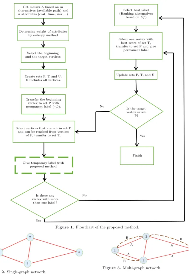
This process is shown in the owchart in Figure 1.
4. Numerical examples 4.1. Example 1
In Figure 2, there is a network with 4 nodes with a single path between each 2 of them which are shown with lines. Each of these paths has attributes, such as cost, distance, time, and risk, given in Table 1. In Table 2, the weights of each attribute are available. The aim is to nd the shortest path between 1 and 4.
The weighting of attributes is done by entropy method. Then, according to the beginning and target vertices, sets P, T, and U are dened and Table 3 is completed. First, the beginning vertex takes a permanent label ({,0). Two paths 1-2 and 1-3 have the passing conditions such that vertex 2 is rated as 0.8343 and vertex 3 is rated as 0.1657 based on the TOPSIS method, and the temporary labels (1,1) and (1,2) are obtained for 2 and 3, respectively. According to the second component of temporary label which shows the
Table 1. The parameters of each path. Path Cost Time Risk
1-2 20 20 4
1-3 13 45 3
2-3 17 30 5
2-4 20 20 2
3-4 20 10 2
Table 2. The weight of attributes by Entropy method. Attributes Cost Time Risk
w 0.0659 0.5863 0.3478
Table 3. The proposed method of implementation process (Example 1).
Step Set Label
P T U
0 1,2,3,4
1 1 2,3 4 2(1,1), 3(1,2)
2 1,2 3,4 3(1,1), 3(2,3), 4(2,2)
3 1,2,3 4 4(2,1), 4(3,2)
4 1,2,3,4
The nal route: 1-2-4 The nal objective function: (40,40,6)
priority, path 1-2 is are selected. Therefore, vertex 2 has a permanent label and is transferred to set P. Paths 2-4, 2-3, and 1-3 have the ability to get a permanent label for the next move. It should be noted that for routes 2-4 and 2-3, the values of the attributes must be aggregated by the values of 1-2. Repeating TOPSIS solution for these three paths results in 0.8559 and 0.0163 points for vertex 3 and in 0.5367 for vertex 4. So, temporary labels (1,1) and (2,3) are obtained for vertex 3 and (2,2) for vertex 4. According to the second component of temporary label which shows the priority, path 1-3 is selected. Paths 2-4, 2-3, and 3-4 have the ability to get a permanent label for the next move. According to the ranks, path 2-4 will be selected; so, we nally reach the destination node. So, the optimal path is 1-2-4 which has the nal objective function (40-40-6).
4.2. Example 2
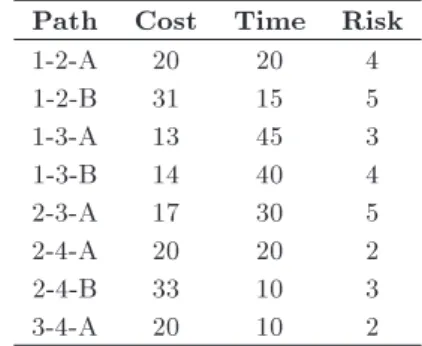
Other conditions could also be considered in which there is more than one direct path to get from one vertex to another vertex (Figure 3). The following example considers the multi-path condition of the above examples. Each of these paths has attributes such as cost, distance, time, and risk, given in Table 4. In Table 5, the weights of each attribute are available. The aim is to nd the shortest path between 1 and 4.
Table 4. The parameters of each path. Path Cost Time Risk
1-2-A 20 20 4
1-2-B 31 15 5
1-3-A 13 45 3
1-3-B 14 40 4
2-3-A 17 30 5
2-4-A 20 20 2
2-4-B 33 10 3
3-4-A 20 10 2
Table 5. The weight of attributes by entropy method. Attributes Cost Time Risk
Figure 1. Flowchart of the proposed method.
Figure 2. Single-graph network.
The weighting of the attributes is done by entropy method. Then, according to the beginning and target vertices, sets P, T, and U are dened and Table 6 is completed. As mentioned earlier, rst, the beginning
Figure 3. Multi-graph network.
vertex 1 will get a permanent label. Then, Four paths 1-2-A, 1-2-B, 1-3-A, and 1-3-B should be checked between the existing conditions. With the TOPSIS solution, values 0.7956, 0.7491, 0.2509, and 0.2783 can be calculated for the mentioned routes, respectively.
Table 6. The proposed method of implementation process (Example 2).
Step Set Label
P T U
0 1,2,3,4
1 1 2,3 4 2A(1,1), 2B(1,2), 3A(1,4), 3B(1,3) 2 1,2 3,4 3A(1,2), 3B(1,1), 3A(2,5), 4A(2,4), 4B(2,3)
3 1,2,3 4 4A(2,2), 4B(2,1), 4A(3,3)
4 1,2,3,4
The nal route: 1(A)-2(B)-4 The nal objective function: (53,30,7)
Temporary labels (1,1), (1,2), (1,4), and (1,3) will be given to the vertices and ultimately 1-2-A will be selected. Now, paths 2-3-A, 2-4-A, 2-4-B, 1-3-A, and 1-3-B should be compared. By reapplying TOPSIS, values 0.2049, 0.4441, 0.4901, 0.6306, and 0.7060 will be obtained and the labels will be: A,5), A,4), (2-B,3), (1-A,2), and (1-B,1). Paths 2-4-A, 2-4-B, and 3-4-A should be compared. By reapplying TOPSIS, values 0.5822, 0.6936, and 0.3794 will be obtained and the labels will be: (2-A,2), (2-B,1), (3-A,3). So, according to rating, path 2-4-B should be selected. So, the nal path is 1(A)-2(B)-4 with label (53,30,7).
4.3. Example 3
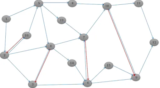
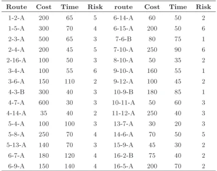
In Figure 4, there is a complex network with 16 nodes and the allowed paths in between which are shown with lines. Each of these paths has attributes, such as cost, distance, time, and risk, given in Table 7.
In Table 8, the weights of each attribute are available by Entropy method. The aim is to nd the shortest path between 1 and 12. Table 9 describes the steps of the proposed method. So, the nal path is 1-5-8-10-11-12.
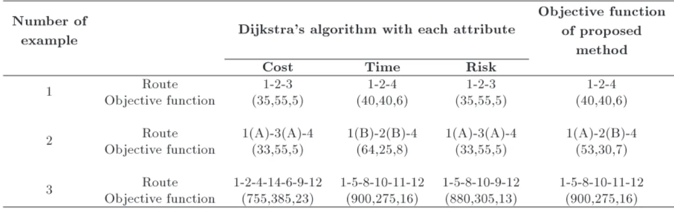
5. Comparing the proposed algorithm with Dijkstra's algorithm
In this section, the results of the proposed model are compared with those of Dijkstra's algorithm that considers each attribute. The results show that the answers are dierent and more ecient according to the weights of attributes. The comparison results are shown in Table 10. According to the results of the proposed algorithm, it can be seen that the weights are assigned to each attribute and the answers have been of eective improvement for the attribute. The attribute with more weight is more important for reducing the costs. If weight of one attribute is 1 and those of the other attributes are 0, the answer to the proposed model is the same with that of single-attribute Dijkstra. So, this method is the extension of single-attribute Dijkstra that is more ecient and more eective.
6. Conclusion
According to complexity of the road networks and the importance of cost and time of travel, choosing the
Table 7. The parameters of each path.
Route Cost Time Risk route Cost Time Risk
1-2-A 200 65 5 6-14-A 60 50 2
1-5-A 300 70 4 6-15-A 200 50 6
2-3-A 500 65 3 7-6-B 80 75 1
2-4-A 200 45 5 7-10-A 250 90 6
2-16-A 100 50 3 8-10-A 50 35 2
3-4-A 100 55 6 9-10-A 160 55 1
3-6-A 150 110 2 9-12-A 100 45 2
4-3-B 300 40 3 10-9-B 180 85 1
4-7-A 600 30 3 10-11-A 50 60 3
4-14-A 35 40 2 11-12-A 250 40 3
5-4-A 100 100 3 13-7-A 30 20 3
5-8-A 250 70 4 14-6-A 70 50 5
5-13-A 140 70 3 15-9-A 45 30 2
6-7-A 180 120 4 16-2-B 75 40 2
6-9-A 150 140 4 16-5-A 200 70 2
Table 8. The weight of attributes by entropy method. Attributes Cost Time Risk
W 0.5563 0.2081 0.2352
shortest path between two points is considered as one of the vital issues. In this article, we attempted to combine Dijkstra's algorithm and TOPSIS method to have a proper selection based on the given priorities.
This combined approach is called multi-attributes Di-jkstra method. In this method, according to the weight of each attribute, suitable performance was applied for determining the nal route between two specic nodes. Using comparison data of this method with the single-attribute Dijkstra, the eciency of the proposed method was examined. Importance of attributes can be observed with their allocated weights. In the future research, we can use more attributes due to the
in-Table 9. The proposed method of implementation process (Example 3).
Step Set Label
P T U
0 1,2,3,4,...,16
1 1 2,5 3,4,6,...,16 2(1,1), 5(1,2)
2 1,2 3,4,5,16 6,...,15 3(2,4), 4(2,3), 5(1,1), 16(2,2)
3 1,2,5 3,4,8,13,16 6,7,9,..,15 3(2,6), 4(2,3), 16(2,1), 4(5,2), 8(5,5), 13(5,4) 4 1,2,5,16 3,4,8,13 6,7,9,..,15 3(2,5), 4(2,2), 4(5,1), 8(5,4), 13(5,3) 5 1,2,4,5,16 3,7,8,13,14 6,9,10,11,12 3(2,4), 3(4,5), 7(4,6), 14(4,2), 8(5,3), 13(5,1) 6 1,2,4,5,13,16 3,7,8,14 6,9,10,11,12 3(2,3), 3(4,4), 14(4,2), 13(7,1) 7 1,2,4,5,7,13,16 3,6,8,10,14 9, 11,12 3(2,4), 3(4,5), 14(4,1), 8(5,2), 6(7,3), 10(7,6)
8 ... ... ... ...
9 ... ... ... ...
10 ... ... ... ...
... ... ... ... ...
14 1,2,3,4,5,6,7,8,9,10,11,12,13,14,15,16 ... ... ...
The nal route: 1-5-8-10-11-12 The nal objective function: (900,275,16)
Table 10. The results of comparison of the proposed algorithm with Dijkstra's algorithm. Number of
example Dijkstra's algorithm with each attribute
Objective function of proposed
method
Cost Time Risk
1 Objective functionRoute (35,55,5)1-2-3 (40,40,6)1-2-4 (35,55,5)1-2-3 (40,40,6)1-2-4 2 Objective functionRoute 1(A)-3(A)-4(33,55,5) 1(B)-2(B)-4(64,25,8) 1(A)-3(A)-4(33,55,5) 1(A)-2(B)-4(53,30,7)
3 Objective functionRoute 1-2-4-14-6-9-12(755,385,23) 1-5-8-10-11-12(900,275,16) 1-5-8-10-9-12(880,305,13) 1-5-8-10-11-12(900,275,16)
creasing importance of the pollution issues in dierent routing conditions, and we can use this method and consider the emissions and fuel consumption costs as one of the attributes. In addition, the algorithm can be developed for determining the best and most ecient path between any two nodes on the network. In other words, instead of having a specic beginning node and a specic target node, this algorithm is applied to all nodes. Stochastic and uncertain conditions can be used to simulate the real world. The algorithm can also be developed in dierent vehicle routing problems as for future studies.
References
1. Delling, D., Sanders, P., Schultes, D. and Wagner, D. \Engineering route planning algorithms", In Algorith-mics of Large and Complex Networks, Springer Berlin Heidelberg, pp. 117-139 (2009).
2. Chen, D.Z. \Developing algorithms and software for geometric path planning problems", ACM Computing Surveys (CSUR), 28(4es), p. 18 (1996).
3. Knuth, D.E. \A generalization of Dijkstra's algo-rithm", Information Processing Letters, 6(1), pp. 1-5 (1977).
4. Dljkstra, E.W. \A note on two problems in connexion with graphs", Numer. Math, 1, pp. 269-271 (1959). 5. Bang-Jensen, J. and Gutin, G.Z. \Digraphs: Theory,
Algorithms and Applications", Springer Science & Business Media (2008).
6. Zeng, W. and Church, R.L. \Finding shortest paths on real road networks: the case for A", Int. J. of
Geographical Information Science, 23(4), pp. 531-543 (2009).
7. Hart, P.E., Nilsson, N.J. and Raphael, B. \A formal basis for the heuristic determination of minimum cost paths", Systems Science and Cybernetics, IEEE Transactions on, 4(2), pp. 100-107 (1968).
8. Rivest, R.L. and Leiserson, C.E., Introduction to Algorithms, McGraw-Hill, Inc (1990).
9. Rosen, K.H., Discrete Mathematics and Its Applica-tions, McGraw-Hill., Boston, MA (2003).
10. Stein, C., Cormen, T., Rivest, R. and Leiserson, C., Introduction to Algorithms, 3, Cambridge, MA: MIT Press (2001).
11. Black, P.E., Johnson's algorithm, Dictionary of Al-gorithms and Data Structures, National Institute of Standards and Technology (2004).
12. Hwang, C.L. and Yoon, K., Multiple Attributes Decision Making Methods and Applications, Berlin: Springer (1981).
13. Benitez, J.M., Martin, J.C. and Roman, C. \Using fuzzy number for measuring quality of service in the hotel industry", Tourism Management, 28(2), pp. 544-555 (2007).
14. Wang, Y.M. and Elhag, T.M.S. \Fuzzy TOPSIS method based on alpha level sets with an application to bridge risk assessment", Expert Systems with Appli-cations, 31, pp. 309-319 (2006).
15. Triantaphyllou, E. and Lin, C.T. \Development and evaluation of ve fuzzy multi attribute decision-making methods", Int. J. Approx Reason, 14, pp. 281-310 (1996).
16. Chen, C.T. \Extensions of the TOPSIS for group decision making under fuzzy environment", Fuzzy Sets Syst., 114, pp. 1-9 (2000).
17. Tsaur, S.H., Chang, T.Y. and Yen, C.H. \The eval-uation of airline service quality by fuzzy MCDM", Tourism Management, 23(2), pp. 107-115 (2002). 18. Byun, H.S. and Lee, K.S. \A decision support system
for the selection of a rapid prototyping process using the modied TOPSIS method", Int. J. of Adv. Manuf. Tech., 26, pp. 1338-1347 (2006).
19. Wang, Y.J. \Applying FMCDM to evaluate nancial performance of domestic airlines in Taiwan." Ex-pert Systems with Applications, 34(3), pp. 1837-1845 (2008).
20. Ertugrul, _I. and Karakasoglu, N. \Comparison of fuzzy AHP and fuzzy TOPSIS methods for facility location selection", The International Journal of Ad-vanced Manufacturing Technology, 39(7-8), pp. 783-795 (2008).
21. Ertugrul, _I. and Karakasoglu, N. \Performance evalu-ation of Turkish cement rms with fuzzy analytic
hier-archy process and TOPSIS methods", Expert Systems with Applications, 36(1), pp. 702-715 (2009).
22. Feng, X. \TOPSIS method for hesitant fuzzy multiple attribute decision making", J. Intell. Fuzzy Syst., 26(5), pp. 2263-2269 (2014).
23. Tor, F., Farahani, R.Z. and Mahdavi, I. \Fuzzy MCDM for weight of object's phrase in location rout-ing problem", Applied Mathematical Modellrout-ing (2015). 24. Chabrier, A. \Vehicle routing problem with elementary shortest path based column generation", Computers & Operations Research, 33(10), pp. 2972-2990 (2006). 25. Felner, A., Stern, R., Ben-Yair, A., Kraus, S. and
Netanyahu, N. \PHA*: nding the shortest path with A* in an unknown physical environment", Journal of Articial Intelligence Research, 21, pp. 631-670 (2004).
26. Azi, N., Gendreau, M. and Potvin, J.Y. \An exact algorithm for a single-vehicle routing problem with time windows and multiple routes", European Journal of Operational Research, 178(3), pp. 755-766 (2007). 27. Donati, A.V., Montemanni, R., Gambardella, L.M.
and Rizzoli, A.E. \Integration of a robust shortest path algorithm with a time dependent vehicle routing model and applications", In Computational Intelligence for Measurement Systems and Applications, IEEE Inter-national Symposium on, pp. 26-31 (2003).
28. Lee, C.G., Epelman, M.A., White, C.C. and Bozer, Y.A. \A shortest path approach to the multiple-vehicle routing problem with split pick-ups", Transportation Research Part B: Methodological, 40(4), pp. 265-284 (2006).
29. Prim, R.C. \Shortest connection networks and some generalizations", Bell System Technical Journal, 36(6), pp. 1389-1401 (1957).
30. Cherkassky, B.V., Goldberg, A.V. and Radzik, T. \Shortest paths algorithms: Theory and experimental evaluation", Math. Prog., 73, pp. 129-174 (1996). 31. Gallo, G. and Pallottino, S. \Shortest paths
algo-rithms", Annals of Operations Research, 13, pp. 3-79 (1988).
32. Eklund, P.W., Kirkby, S. and Pollitt, S. \A dynamic multi-source Dijkstra's algorithm for vehicle routing", In Intelligent Information Systems, Australian and New Zealand Conference on, pp. 329-333, IEEE (1996). 33. Peyer, S., Rautenbach, D. and Vygen, J. \A gener-alization of Dijkstra's shortest path algorithm with applications to VLSI routing", Journal of Discrete Algorithms, 7(4), pp. 377-390 (2009).
34. Wen, L., Catay, B. and Eglese, R. \Finding a minimum cost path between a pair of nodes in a time-varying road network with a congestion charge", European J. of Operational Research, 236(3), pp. 915-923 (2014). 35. Deng, Y., Chen, Y., Zhang, Y. and Mahadevan, S.
\Fuzzy Dijkstra algorithm for shortest path problem under uncertain environment", Applied Soft Comput-ing, 12(3), pp. 1231-1237 (2012).
36. Chen, Y.Z., Shen, S.F., Chen, T. and Yang, R. \Path optimization study for vehicles evacuation based on Dijkstra algorithm", Procedia Engineering, 71, pp. 159-165 (2014).
37. Vidal, T. \General solution approaches for multi-attribute vehicle routing and scheduling problems". 4OR, 12(1), pp. 97-98 (2014).
38. Yin, C.Z., Bu, L. and Gong, H.T. \Mathematical model and algorithm of split load vehicle routing prob-lem with simultaneous delivery and pickup", Interna-tional Journal of Innovative Computing, Information and Control, 9(11), pp. 4497-4508 (2013).
39. Vidal, T., Crainic, T.G., Gendreau, M. and Prins, C. \Heuristics for multi-attribute vehicle routing prob-lems: a survey and synthesis", European Journal of Operational Research, 231(1), pp. 1-21 (2013). 40. Vidal, T., Crainic, T.G., Gendreau, M. and Prins,
C. \A unied solution framework for multi-attribute vehicle routing problems", European Journal of Oper-ational Research, 234(3), pp. 658-673 (2014).
41. Sicilia, J.A., Quemada, C., Royo, B., and Escun, D. \An optimization algorithm for solving the rich vehicle routing problem based on variable neighbor-hood search and Tabu search metaheuristics", Journal of Computational and Applied Mathematics, 291, pp. 468-477 (2016)
42. Dayarian, I., Crainic, T.G., Gendreau, M. and Rei, W. \A column generation approach for a multi-attribute vehicle routing problem", European Journal of Opera-tional Research, 241(3), pp. 888-906 (2015).
43. Wei-qin, W., Yu, T., Jing, Q. and Qi-zhen, W. \An improved label heuristic algorithm for multi-attribute vehicle routing problem", In Management Science and Engineering (ICMSE), International Conference on, pp. 248-257, IEEE (2013).
Biographies
Emad Roghanian received his PhD degree from Iran University of Science and Technology, Tehran, Iran, in 2006. He is currently an Associate Professor in the Fac-ulty of Industrial Engineering at K.N. Toosi University of Technology. His research interests include supply chain management, project management, probability models, and applied operations research. He has au-thored numerous papers presented at conferences and published in journals, including Applied Mathematical Modelling, Computers & Industrial Engineering and Applied Mathematics and Computation.
Zohreh Shakeri Kebria received her BSc degree in Industrial Engineering from K.N. Toosi University of Technology in 2014. Presently, she is a master student in Industrial Engineering at K.N. Toosi University of Technology. Her related area ranges from vehicle routing problems to logistics and to supply chain management.