Sharif University of Technology
Scientia IranicaTransactions B: Mechanical Engineering www.scientiairanica.com
Comparison of ISPH and WCSPH methods to solve
uid-structure interaction problems
H. Sabahi and A.H. Nikseresht
Department of Mechanical Engineering, Shiraz University of Technology, Shiraz, P.O. Box 71555-313, Iran. Received 3 November 2014; received in revised form 21 December 2015; accepted 8 February 2016
KEYWORDS Incompressible Smoothed Particle Hydrodynamics (ISPH);
Hypo-elastic gate; Fluid-solid interaction.
Abstract.In this paper, the in-house code based on the smoothed particle hydrodynamics is proposed to simulate a Fluid-Solid Interaction (FSI) problem. This method is a Lagrangian, mesh-free method, and it has a high ability to capture the free surface in two-phase ows and also the interface in FSI problems. To compare Weakly Compressible SPH (WCSPH) and Incompressible SPH (ISPH) schemes, uid ow under a hypo-elastic gate is simulated in solid and uid domains with both methods. At rst, uid domain is simulated with ISPH method and solid domain is solved with WCSPH scheme. Another simulation is done with both uid and solid parts solved by WCSPH method. The results of both methods are in good agreement with each other and also with other researcher's results. So, it is concluded that it is easier to model the uid ow with ISPH scheme and the solid part with WCSPH in coupling uid-solid interaction problems with good accuracy.
© 2016 Sharif University of Technology. All rights reserved.
1. Introduction
The interaction of a moveable or deformable structure with an internal or external uid ow is called Fluid-Solid Interaction (FSI). Hydrodynamic damping of oshore structures in wave, oscillation of aircraft wings, and the ow of blood through arteries are some well-known examples of such phenomena.
The arbitrary Lagrangian Eulerian [1] and the Coupled Eulerian Lagrangian (CEL) methods are the most popular methods to solve the FSI problems. In both methods, Eulerian and Lagrangian formulations are coupled to obtain the advantages of each pure method and prevent the disadvantages of each un-coupled formulations. In problems with small defor-mation, ALE methods have high accuracy and low computational cost, but in the problems of large
de-*. Corresponding author. Tel./Fax: +98 71 37264102; E-mail addresses: [email protected] (H. Sabahi); [email protected] (A.H. Nikseresht)
formation, these coupled methods need the re-meshing procedure and re-meshing has high computational cost. Smoothed Particle Hydrodynamics (SPH) is a mesh-free, Lagrangian and particle adaptive method which has a high ability to solve the large deformation uid-solid interaction problems. This method has a good ability to track the free surface and nd the interface in FSI problems. Easy implementation of SPH group methods for solving uid ows around complex geome-tries is another advantage of these schemes.
There are two approaches in the SPH method to nd the pressure of the particles; one is the use of Weakly Compressible SPH (WCSPH) idea, in which an equation of state is solved to nd the pressure. Another approach is Incompressible SPH (ISPH) which is introduced by Cummins and Rudman [2], and in which incompressibility is enforced by solving Poisson equation. It seems that solving the Poisson equation in ISPH method decreases computational speed in each time step, but it should be noted that in WCSPH method, the speed of sound is used to satisfy the
CFL condition and it leads to much smaller time steps in comparison with the ISPH method and more computational cost [3].
The SPH method was rst introduced in astro-physics by Lucy [4] and also by Gingold and Mon-aghan [5]. Nowadays, this method is used to study dierent problems such as interfacial ows, that is, ow elds with dierent uids separated by sharp interfaces [6], free surface and viscoelastic free surface ows [7-9], multi-uid ows [10], wave interactions with porous media [11], and incompressible ows in general [12].
Recently, dierent algorithms of the SPH method are used to solve FSI problems. Antoci et al. [13] used a standard SPH method to model uid-structure inter-action problems. They neglected the eect of viscosity and used a repulsive force to prevent the penetration of uid particles into the solid particles. Yang et al. [14] used a combined SPH-FEM model to simulate FSI problems. ISPH method is also utilized to solve some FSI problems by Raee and Thiagarajan [15]. They used Antoci's model for coupling conditions on the interface, and they also considered the viscosity of uid. The motivation of this work is to show the merits of the ISPH method. For this purpose, the in-house code is implemented based on SPH method. The uid ow in a uid-structure problem is solved by both ISPH and WCSPH methods. In both algorithms, the motion of the solid structure is modeled with WSCPH method. The results and methods of implementation in both algorithms are compared with each other.
2. Governing equations and numerical method 2.1. Governing equations
The equations of motion for two dimensional problems in the Lagrangian description include the conservation of mass and momentum which are as follows:
D
Dt = r:~v; (1)
Dvi
Dt = 1
@ij
@xj + fi; (2)
where t; ; v; f, and are time, density, velocity vector, external force, and stress tensor, respectively. The indices i and j refer to the ith and jth components of a vector. For uids, the stress tensor can be decomposed into isotropic pressure, P , and shear stress, , as follows:
ij = P ij+ ij: (3)
The shear stress for Newtonian uid is as follows: 1 r: i = r2~v
i
; (4)
where is the dynamic viscosity.
Eqs. (1) and (2) are also valid for solids. The stress tensor can be decomposed into isotropic pressure, P , and deviatoric shear stress tensor:
ij = P ij+ Sij; (5)
where is the Kronecker delta. The deviatoric shear stress tensor can be obtained from Eq. (6) [16]:
DSij
Dt =2s
Dij 13Dmmij
+SikWjk+SkjWik;(6)
where s, D, and W are the shear modulus, rate of
deformation tensor, and spin tensor, respectively. D and W can be obtained from Eqs. (7) and (8):
Dij =12
@v
i
@xj +
@vj
@xi
; (7)
Wij= 12
@vi @xj @vj @xi : (8)
2.2. Introduction to SPH
The SPH method is based on the integral interpolation theory. The value of any function in the SPH method is obtained by the values of the neighboring particles. Eq. (9) is the main idea in the SPH method [2]:
f(x) = Z
f (x0) (x x0) dx0; (9)
where is the Kronecker delta. The continuous domain should be discretized, and the smoothing kernel function (w) is used instead of and the domain is represented by some particles, so the function f(x) can be represented as:
hf(x)ia =XN
j=1
mb
bf(xb)w(x xb; h); (10)
where m is the mass of particles, h is the smoothing length which denes the inuence domain of the weight function, N is the number of neighboring particles, and indices a and b represent the central particle and its neighboring, respectively. The smoothing kernel function should have the following properties:
8 > > > < > > > : lim
x!x0w(x x
0)dx0= (x x0)
w(x x0) = 0 jx x0j > kh
R
w(x x0)dx0 = 1
(11)
In addition, the rst and second derivatives should exist.
The stability of the SPH algorithm is dependent on the second derivative of the kernel function [17]. In
this paper, the cubic spline smoothing kernel function with the following formulation is used [15,18]:
w(r; h) = 8 > > > < > > > : 10
7h2 1 32R2+34R3
R < 1
10
28h2(2 R)3 1 R 2
0 R > 2
(12)
where R = r
h, r is the distance between particles, h
is set to h = 1:3dx, and dx is the initial horizontal distance between two neighboring particles. According to Eq. (12), particle b is a neighbor for particle a if rab< 2h.
2.3. SPH approximation of divergence, gradient, and Laplasian operators
Divergence of the vector ~V and gradient of a function f(x) can be obtained as follows [19]:
r:~V t =
N
P
b=1mb
~Va ~Vb
:raWab
t ; (13)
hrf(xa)i = a N
X
b=1
mb
f(xb)
2 b +
f(xa)
2 a
rawab; (14)
in which:
rawab=
@w @rab
xa xb
jrabj ;
@w @rab
ya yb
jrabj
: (15)
The SPH approximation of Eq. (4) is:
r2~v
a=
X
b
4mb(a+ b)~rab:rawab
(a+ b)2
jrabj2+ 2
(~va ~vb) ;
(16) where = 0:1h is a non-zero parameter to prevent the denominator from getting zero.
2.4. SPH approximation of continuity and momentum equations
According to Eq. (10), the density can be found as follows:
a= N
X
b=1
bwmb b =
N
X
b=1
wmb: (17)
Another form of density variation which is found from continuity equation can be written as in Eq. (18):
da
dt = a
N
X
b=1
mb
b(ua ub):rawab: (18)
According to Eqs. (16) and (14), the SPH approxima-tion of the momentum Eq. (2) for uid can be obtained
as: Dvai
Dt = X
bmb
Pa 2 a + Pb 2 b @wab
@axi
+X
b
4mb(a+b)~rab:rawab
(a+b)2
jrabj2+2
(~vai ~vbi)+fi:
(19) Generally, in the SPH method, there are two schemes to nd the pressure. The pressure in the standard form of the SPH is obtained from an equation of state; this form is called Weakly Compressible SPH (WCSPH). The equation of state for both parts (uid and solid) has the form of Eq. (20):
P = c2
0( 0): (20)
In the solid, c2
0= k0 where k is the bulk modulus and
for the uid, c2
0 = 0 where is the compressibility
modulus where 0 is the reference density. The
WCSPH method cannot satisfy incompressibility, there is another form of SPH to satisfy incompressibility, and this form is called Incompressible SPH (ISPH). In the ISPH method, pressure is obtained from the Poisson equation, and the continuity equation is satised by vanishing velocity divergence. The Poisson equation can be found as [2]:
r:
1 rPt+1
= r:~vt: (21)
The left-hand side of Eq. (21) is discretized as fol-lows [10,20]: r: 1 rP a= N X b
mb( 8 a+b)2
(Pa Pb)~rab:rawab
jrabj2+2 (22);
where ~rab= ~ra ~rb. The momentum equation for solid
particles can be written as: Dvai
Dt = X
b
mb P2a a + Pb 2 b + Y ab ! @wab
@axi
+X b mb Sija 2 a + Sijb 2
b +(Rija+Rijb)f n@wab
@axj+f(23)i;
whereQ
abis an articial viscosity and Rij is an articial
stress, these two terms have been introduced in order to solve numerical problems. Q
ab has been proposed
by [21] and can smooth out the velocity oscillations when particles get too close to each other:
Y ab = 8 < :
cabab
ab ~vab:~rab< 0
0 ~vab:~rab> 0
where:
~rab= ~ra ~rb;
~vab= ~va ~vb;
ab= h (~vab:~rab)
jrabj2+ 0:01h2;
ab= 12(a+ b); and cab= 12(ca+ cb):
c is the speed of sound and is an articial viscosity coecient. According to the following equations, the component of Rij can be obtained:
Rxx a = 8 < :
exxa
2
a
xx a > 0
0 xx a < 0
(25) Ryy a = 8 < :
eayy
2
a
yy a > 0
0 yy a < 0
(26)
To obtain Rij, it is necessary to nd principal
stresses [16]:
xx
a = c2xxa + 2scaxy+ s2ayy; (27)
yy
a = s2xxa + 2scaxy+ c2yya ; (28)
where c and s represent cos and sin , and:
tan 2a = 2 xy a
xx
a ayy; (29)
Rxx a = 8 < :
exxa
2
a
xx a > 0
0 xx a < 0
(30) Ryy a = 8 < :
eayy
2
a
yy a > 0
0 yy a < 0
(31)
e is a constant and is set to e = 0:3. Rxx
a = c2Rxxa + s2Ryya ; (32)
Ryy
a = s2Rxxa + c2Ryya ; (33)
Rxy
a = cs Rxxa Ryya
: (34)
f = wij
w(l0;h) where l0 is the initial distance between two
neighboring particles, and n is set to 4.
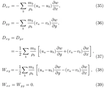
Eqs. (7) and (8) are discretized in order to found deviatoric stress tensor.
Dxx=
X
b
mb
b(ua ub)
@w
@x; (35)
Dyy =
X
b
mb
b (va vb)
@w
@y; (36)
Dxy= Dyx
= 12X
b
mb
b
(ua ub)@w@y+(va vb)@w@x
;
(37)
Wxy= 12
X
b
mb
b
(ua ub)@w@y (va vb)@w@x
; (38)
Wxx= Wyy = 0: (39)
Finally, the components of deviatoric stress tensor can be found as:
Sijn+1 Sn ij
t =2s
Dn
ij 13Dmmn ij
+ Sn+1
ik Wjkn + Skjn+1Wikn: (40)
2.5. Free surface and wall boundary condition The base rule of nding free surface interface in the SPH methods is the variation of density near the free surface. Due to the fact that the surface particles in free surface have less neighboring particles, the density of these particles decreases according to Eq. (17), as depicted in Figure 1. Therefore, a particle is considered in the free surface if < 0where 0:8 < < 0:99 [22].
In this research, dummy particles are used to prevent the penetration of uid particles into the solid particles in the wall boundary conditions. This method was purposed by Koshizuka et al. [23]. Two sets of particles are used in this method; the rst set of particles are placed on the boundary as shown in Figure 2, and the second set of particles are used
Figure 2. Three rows of dummy particles in the boundary.
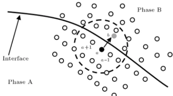
Figure 3. Interface and its normal vector.
to avoid density change close to the boundary. The Poisson equation is solved to calculate the pressure of dummy particles and the velocity is set to zero. 2.6. Fluid-solid interaction model
In the SPH method, each particle has a support domain. All particles with the distance of 2h or lower than 2h are in the support domain of the central particle. In FSI problems, there are two sets of particles (uid and solid) close to the interface. Thus, the support domain of the interface particles included both solid and uid particles (like particles a and b in Figure 3). By extending the summation of Eqs. (19) and (23) to all particles regardless of their nature, the coupling condition can be satised [13].
In the previous works, some repulsive forces were used to prevent the penetration of uid particles into the solid particles [13,14,24]. The previously used repulsive forces are complex and are sometimes dependent on the uid particles pressure. In the present work, a new repulsive force is introduced that is very easy to implement and it is not dependent on pressure. This repulsive force was rst proposed by Esmaeili [25] for wall boundary condition. This force works as an external force and exert from solid particles to the uid particles. Also, the dynamic interface condition is satised by exerting the repulsive
force on the opposite direction to solid particles [14]. This new repulsive force which is used in the present FSI problem with WCSPH method can be depicted as follows:
f = 8 > < > :
1 3
!
ut 1:~n
dt 1 0:5q0:5q
~u:~n < 0 0 ~u:~n > 0
(41)
where q = jrijj
2h (0 < q < 1) and ~n is the normal to
the interface particles. The tangential vector of solid particles which are near to the interface can be found as in [26]:
bta = (tax; tay) =
x
a+1 xa 1
jra+1;a 1j ;
ya+1 ya 1
jra+1;a 1j
; (42)
where a 1 and a + 1 represent the two particles which are before and after the particle a, respectively, as is shown in Figure 3. The vertical vector at particle a can be found as:
~na= ( tay; tax): (43)
In a few papers, the ISPH method was used to simulate FSI problems [15]. In this method, incompressibility is satised by the Poisson equation. In this paper, to compare the implementation of WCSPH and ISPH methods, uid particles of a FSI problem are simulated by both WSCPH and ISPH methods. In the ISPH method, there is no need to use the repulsive force, and it is one of the merits of the ISPH method.
In both WCSPH and ISPH methods, to model the uid-solid interaction problems, in each time step, at rst, the uid domain is solved and the uid particles are moved with their calculated velocities. Afterwards, the exerted force by the uid particles on the solid particles are obtained, so the solid domain equation is solved and the solid particles are moved to their new locations. In the WCSPH method, to prevent the penetration of uid particles into the solid domain, a repulsive force is implemented. So, in each time step, the repulsive force is specied and exerted on the uid particles from solid particles; it is also exerted from the uid particles on the solid particles according to the Newtown's third law.
2.7. XSPH velocity correction
In order to smooth out oscillation of particles velocity, the XSPH technique is used. In this technique, particles move with a velocity closer to the average velocity, and particles are moved by [27]:
D~ra
Dt = !va " X
b
mb
ab(!va
!v
b) wab; (44)
2.8. ISPH algorithm
In the ISPH algorithm, a prediction-correction scheme is used for time marching. So, the complete movement of the uid particles is achieved after nishing the two sub steps of each time step. In the prediction step, particles move without sensing the eect of pressure gradient and the temporal particle position, and velocity can be founded by solving the momentum equation only by considering the body and shear forces with the following equations [2]:
~r= ~rt+ ~vtt; (45)
~v=
~g +r2~vt; (46)
~v= ~vt+ ~v; (47)
where subscripts t and denote the parameters at time t and in the prediction step. After nding the position and velocity in the prediction step, the density in this step can be obtained from Eq. (17). In the second sub step (correction step), the eect of pressure gradient is considered. The pressure in this new time step (t + 1) can be found by solving the Poisson equation [28]:
r:
1 rPt+1
=r:~vt: (48)
In the correction step, incompressibility is satised, and the position and velocity are corrected as follows:
~vt+1= ~v+ ~v; (49)
~rt+1= ~rt+~vt+ ~v2 t+1t; (50)
where subscript represents the correction step and! v is:
~v= 1
rPt+1t: (51)
3. Results and discussion 3.1. Fluid ow under a gate
To validate the uid part of the prepared code, a uid ow under a gate is solved by the ISPH method, and results are compared with the nite volume and VOF scheme. The uid is water with = 1000 kg
m3,
= 0:001 N
m2s, and g = 9:81 sm2. The geometry
is a tank with the length and the height of 0.1 and 0.14 m, respectively. Also the height of the gate is 0.03 m. In this simulation, the total number of particles is 1689; the initial space between the particles is 0.00375 m, and the time step is set to 0.001 s. To check the independency from the number of particles, this example is also simulated with 2580 particles.
The size of the particles adjacent to the gate is set to 0.001 m. After that, the particles size is set to 0.002 m and adjusted to 0.00375 m far from the gate. The comparison of uid ow under the gate with ISPH and VOF schemes is depicted in Figure 4 for dierent particle sizes and shows similar results with a reasonable agreement. It also shows the ability of the ISPH method to capture the free surface ows [28]. This example is also solved by WCSPH method with 1689 particles.
Figure 5 shows the pressure distribution of uid ow under the gate for two dierent time steps. 3.2. Oscillating plate
For validating the solid part of the code, vibration of an elastic plate is simulated [13,16]. The plate has one end clamped and the other end is free, as is shown in Figure 6. In this example, the plate is initially horizontal and oscillates around the initial position of its fundamental mode (kL = 1:875). According to the analytical expression of the rst normal mode, the initial velocity distribution is:
vy= c0v0Lf(L)f(x); (52)
where:
f(x) =(cos(kL) + cosh(kL))(cosh(kx) cos(kx)) +(sin(kL) sinh(kL))(sinh(kx) sin(kx));(53) and v0L = 0:01 is the initial velocity of the free end
of the plate, and other properties are: L = 0:2 m, H = 0:02 m, = 1000 mkg3, s = 7:15 106 Nm2, and
K = 3:25 106 N
m2. The results are compared with the
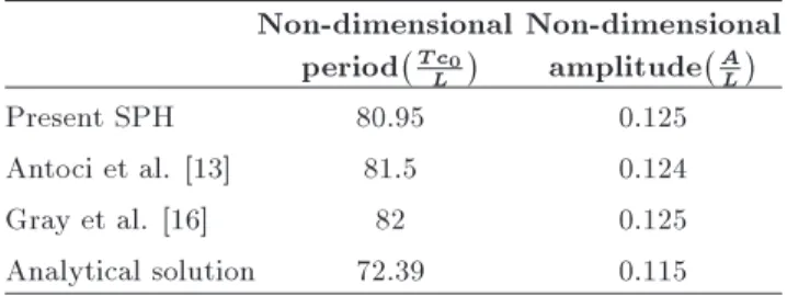
analytical solution and also with the other researchers' results (Table 1).
This example is solved by WCSPH method along with two sets of particles, n = 3195 and n = 5560 particles; the time step is set to t = 10 5 second.
The results are in good agreement with other results as depicted in Figure 7.
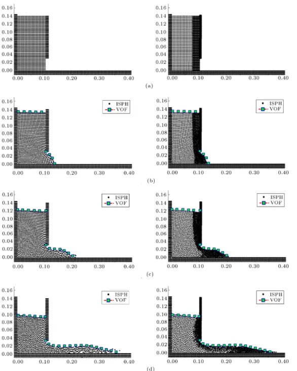
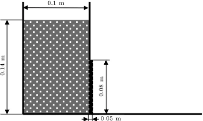
3.3. Fluid ow under a hypo-elastic gate In this part, the deformation of an elastic gate due to water pressure is simulated to show the ability of ISPH method in FSI problems. The elastic gate is clamped
Table 1. Non-dimensional parameters. Non-dimensional
period T c0
L
Non-dimensional amplitude A
L
Present SPH 80.95 0.125
Antoci et al. [13] 81.5 0.124
Gray et al. [16] 82 0.125
Figure 4. The comparison of uid ow under the gate with ISPH and VOF methods at times (a) 0.0 s, (b) 0.05 s, (c) 0.1 s, and (d) 0.2 s (left: 1689 particles and right: 2580 particles).
Figure 6. Geometry of the plate.
Figure 7. Vertical displacement of the free end of the plate by n = 3195 and n = 5560 particles.
Figure 8. Initial conguration and geometry of hypoelastic gate.
at one end and free at the other end. The geometry of this example is shown in Figure 8.
In this example, ISPH method is used to nd the pressure of uid particles, and WCSPH method is used to calculate the pressure of solid particles.
The uid properties are = 1000 kg
m3 and =
0:001 N
m2s. The elastic plate properties are K =
2 107 N
m2, S = 4:27 106 Nm2, and = 1100 mkg3.
The accuracy of the SPH method can be improved by increasing the number of particles, but the computa-tional cost increases by increasing the total number of particles. So, in the present work, smaller particles are used close to the places of high gradient, and bigger particles are used in other parts of the domain. For particles a and b with dierent sizes, the smoothing length is set to h = phahb. In this example, there
are 6672 particles in total. The initial spacing between solid particles is set to 0.001 m, for uid particles close to the gate is set to 0.001 m, and far from the gate is set to 0.002 m. To insure numerical stability, the time step is set to t = 3 10 6 second. Figure 9
shows the comparison of the present results with the results of Antoci et al. [13] with the increment of 0.04 second. The particle clustering near the free surface ow is not seen in this research. It is due to the use of the XSPH scheme which is a method to prevent the particle clustering. The results are in good agreement with each other. This example was also simulated with 4945 particles and the results show no signicant changes. To compare the implementation of WCSPH and ISPH methods, the example is again solved by WCSPH method (in both media, uid and solid) with two sets of particles (6667 and 9069). As mentioned earlier, in the present ISPH method, the repulsive force is not used and this is an advantage of this work; another merit is also the coupling of ISPH and WCSPH methods.
Figure 10 shows the pressure distribution under a hypo-elastic gate for four dierent time steps.
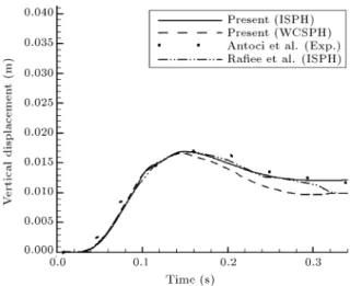
Figures 11 and 12 show the comparison of the present horizontal and vertical displacement compo-nents of the free end of the plate with the experimental results of Antoci et al. [13] and numerical results of Raee et al. [15].
Figures 11 and 12 depict that both ISPH and WCSPH methods have reasonable accuracy, but the ISPH method, especially in vertical displacement, shows higher accuracy. The higher accuracy of ISPH method is due to solving Poisson equation for nding the pressure distribution; therefore, it does not need to use a repulsive force. Furthermore, the number of particles used in the ISPH method is less than the number of particles used in the WCSPH method (4945 particles versus 6667 particles).
Figures 11 and 12 show that ISPH method of Raee's work has also higher accuracy with respect to WCSPH method. Raee et al. [15] used the complex in-tegral method algorithm of Antoci et al. [13] in coupling the FSI problem, and they also used a highly pressure-dependent formulation in their repulsive force. But, in the present work, a simple coupling of FSI problem without using any repulsive force in ISPH method is used, and the results show good agreement with the experiments, especially in the vertical displacement. On the other hand, Raee et al. simulated the problem with 6928 particles, but only 4945 particles are used in the present work.
4. Conclusion
In the present work, both the WCSPH and ISPH methods are used to solve the uid part, and the
Figure 9. Comparison of the present study with the results of Antoci et al. [13] with increment of 0.04 second from t = 0 s.
Figure 10. The pressure distribution of uid ow under a hypo-elastic gate: (a) 0.054 s; (b) 0.117 s; (c) 0.207 s; and (d) 0.288 s.
WCSPH method is used to solve the solid part of a FSI problem. In the WCSPH method, an easy repulsive force which is not pressure-dependent is introduced. In the ISPH method, the pressure of uid particles is obtained by solving the Poisson equation, and the in-compressibility is satised, also the uid and solid parts are coupled without using any repulsive force. Results of the present coupling of the ISPH and WCSPH are in
good agreement with other experimental and numerical data. It is shown that the ISPH coupling with WCSPH has higher accuracy with respect to the use of WCSPH method in both uid and solid parts of a FSI problem. Therefore, it is concluded that this coupling without using any repulsive force is very easy to implement and has enough accuracy and robustness to solve the FSI problems.
Figure 11. The horizontal displacement component of the free end of the plate.
Figure 12. The vertical displacement component of the free end of the plate.
References
1. Rugonyi, S. and Bathe, K. \On nite element analysis of uid ows fully coupled with structural interac-tions", CMES- Computer Modeling in Engineering and Sciences, 2(2), pp. 195-212 (2001).
2. Cummins, S.J. and Rudman, M. \An SPH projection method", Journal of Computational Physics, 152(2), pp. 584-607 (1999).
3. Sun, F. \Investigations of smoothed particle hydrody-namics method for uid-rigid body interactions", PhD Thesis, University of Southampton (2013).
4. Lucy, L. \A numerical approach to the testing of fusion processes", The Astronomical J., 82, pp. 1013-1024 (1977).
5. Gingold, R.A. and Monaghan, J.J. \Smoothed par-ticle hydrodynamics-theory and application to non-spherical stars", Monthly Notices of the Royal Astro-nomical Society, 181, pp. 375-389 (1977).
6. Colagrossi, A. and Landrini, M. \Numerical simulation
of interfacial ows by smoothed particle hydrodynam-ics", J. Comput. Phys., 191, pp. 448-475 (2003).
7. Raee, A., Manzari, M.T. and Hosseini, M. \ An incompressible SPH method for simulation of unsteady viscoelastic free-surface ows", Int. J. Non-Linear Mech., 42, pp. 1210-1223 (2007).
8. Shao, S. \Incompressible smoothed particle hydrody-namics simulation of multiuid ows", International Journal for Numerical Methods in Fluids, 69(11), pp. 1715-1735 (2012).
9. Antuono, M., Colagrossi, A., Marrone, S. and Molteni, D. \Free-surface ows solved by means of SPH schemes with numerical diusive 361 terms", Computer Physics Communications, 181, pp. 532-549 (2010).
10. Ghadampour, Z., Talebbeydokhti, N., Hashemi, M.R., Nikseresht, A.H. and Neill, S.P. \Numerical simulation of free surface mudow using incompressible SPH", IJST, Transactions of Civil Engineering, 37, pp. 77-95 (2013).
11. Shao, S. \Incompressible SPH ow model for wave interactions with porous media", Coastal Engineering, 57, pp. 304-316 (2010).
12. Liu, G.R. and Liu, M.B., Smoothed Particle Hydrody-namics: A Meshfree Particle Method, World Scientic Publishing Co. Pte. Ltd. (2003).
13. Antoci, C., Gallati, M. and Sibilla, S. \Numerical simulation of uid-structure interaction by SPH", Computers & Structures, 85(11), pp. 879-890 (2007).
14. Yang, Q., Jones, V. and McCue, L. \Free-surface ow interactions with deformable structures using an SPH-FEM model", Ocean Engineering, 55, pp. 136-147 (2012).
15. Raee, A. and Thiagarajan, K.P. \An SPH projection method for simulating uid-hypo elastic structure in-teraction", Comput. Methods Appl. Mech. Engrg., 198, pp. 2785-2795 (2009).
16. Gray, J., Monaghan, J. and Swift, R. \SPH elastic dynamics", Computer Methods in Applied Mechanics and Engineering, 190(49), pp. 6641-6662 (2001).
17. Morris, J.P., Fox, P.J. and Zhu, Y. \Modeling low Reynolds number incompressible ows using SPH", J. Comp. Phys., 136, pp. 214-226 (1997).
18. Monaghan, J. \Smoothed particle hydrodynamics", Annu. Rev. Astron. Astrophys., 30, pp. 543-574 (1992).
19. Liu, M.L.G. \Smoothed particle hydrodynamics (SPH): An overview and recent developments", Archives of Computational Methods in Engineering, 17, pp. 25-76 (2010).
20. Shao, S. and Lo, E.Y. \Incompressible SPH method for simulating Newtonian and non-Newtonian ows with a free surface", Advances in Water Resources, 26(7), pp. 787-800 (2003).
21. Monaghan, J. and Gingold, R. \Shock simulation by the particle method SPH", Journal of Computational Physics, 52(2), pp. 374-389 (1983).
22. Koshizuka, S. and Oka, Y. \Moving-particle semi-implicit method for fragmentation of incompressible uid", J. Nucl. Sci. Engrg, 123, pp. 421-434 (1996).
23. Koshizuka, S., Nobe, A. and Oka, Y. \Numerical anal-ysis of breaking waves using the moving particle semi-implicit method", International Journal for Numerical Methods in Fluids, 26(7), pp. 751-769 (1998).
24. Schorgenhumer, M., Johannes, A. and Gerstmayr, J. \Smoothed particle hydrodynamics and model-order reduction for ecient modeling of uid-structure in-teraction", 8th Vienna International Conference on Mathematical Modelling - MATHMOD (2015).
25. Esmaili Sikarodi, M.A. \Using GPU in ISPH sim-ulation of incompressible ows", Master of Science Thesis, Departeman of Mechanical and Aerospace Engineering, Shiraz University of Technology (2013) (in Persian).
26. Randles, P. and Libersky, L. \Smoothed particle hy-drodynamics: some recent improvements and applica-tions", Computer Methods in Applied Mechanics and Engineering, 139(1), pp. 375-408 (1996).
27. Monaghan, J. \On the problem of penetration in particle methods", J. Comput. Phys., 82, pp. 1-15 (1989).
28. Ghadampour, Z., Hashemi, M.R., Talebbeydokhti, N., Neill, S.P. and Nikseresht, A.H. \Some numerical aspects of modelling ow around hydraulic structures using incompressible SPH ", Computers and Mathe-matics with Applications, 69, pp. 1470-1483 (2015).
Biographies
Hooshang Sabahi received his BSc degree in Me-chanical Engineering in 2010 from the Islamic Azad University, Shiraz Branch, Iran, and his MSc degree in Mechanical Engineering in 2014 from Shiraz University of Technology, Iran. Now, he is a PhD student of Shiraz University of Technology, Iran. His current research is focused on the SPH method.
Amir Hossein Nikseresht received his BSc, MSc, and PhD degrees from Shiraz University, Shiraz, Iran in 1995, 1997, and 2004, respectively, all in Mechanical Engineering. He is currently an Associate Professor of Mechanical Engineering in Shiraz University of Tech-nology, Iran. His research interests include free surface ows, CFD, hydrodynamics, and mesh-less methods.
![Figure 9. Comparison of the present study with the results of Antoci et al. [13] with increment of 0.04 second from t = 0 s.](https://thumb-us.123doks.com/thumbv2/123dok_us/8380368.2226333/9.892.118.796.151.542/figure-comparison-present-study-results-antoci-increment-second.webp)