Reversible jump MCMC for nonparametric drift estimation for
diffusion processes
Frank van der Meulena, Moritz Schauera,∗, Harry van Zantenb
aDelft Institute for Applied Mathematics (Delft University of Technology). bKorteweg-de Vries Institute for Mathematics (University of Amsterdam).
Abstract
In the context of nonparametric Bayesian estimation a Markov chain Monte Carlo algo-rithm is devised and implemented to sample from the posterior distribution of the drift function of a continuously or discretely observed one-dimensional diffusion. The drift is modeled by a scaled linear combination of basis functions with a Gaussian prior on the co-efficients. The scaling parameter is equipped with a partially conjugate prior. The number of basis function in the drift is equipped with a prior distribution as well. For continuous data, a reversible jump Markov chain algorithm enables the exploration of the posterior over models of varying dimension. Subsequently, it is explained how data-augmentation can be used to extend the algorithm to deal with diffusions observed discretely in time. Some examples illustrate that the method can give satisfactory results. In these examples a comparison is made with another existing method as well.
1. Introduction
Suppose we observe a diffusion process X, given as the solution of the stochastic
dif-ferential equation (SDE)
dXt=b(Xt) dt+ dWt, X0 =x0, (1)
with initial statex0 and unknown drift functionb. The aim is to estimate the drift b when
a sample path of the diffusion is observed continuously up till a time T >0 or at discrete
times 0,∆,2∆, . . . , n∆, for some ∆>0 and n∈N.
Diffusion models are widely employed in a variety of scientific fields, including physics, economics and biology. Developing methodology for fitting SDEs to observed data has therefore become an important problem. In this paper we restrict the exposition to the case that the drift function is 1-periodic and the diffusion function is identically equal to 1. This is motivated by applications in which the data consists of recordings of angles,
cf. e.g. Pokern (2007), Hindriks (2011) or Papaspiliopoulos et al.(2012). The methods we
∗Corresponding author. Address: TU Delft, Mekelweg 4, 2628 CD Delft, The Netherlands. E-mail:
[email protected]. Tel: ++31 15 2782546.
propose can however be adapted to work in more general setups, such as ergodic diffusions with non-unit diffusion coefficients. In the continuous observations case, a diffusion with periodic drift could alternatively be viewed as diffusion on the circle. Given only discrete observations on the circle, the information about how many turns around the circle the process has made between the observations is lost however and the total number of windings is unknown. For a lean exposition we concentrate therefore on diffusions with periodic
drift on R. In the discrete observations setting the true circle case could be treated by
introducing a latent variable that keeps track of the winding number.
In this paper we propose a new approach to making nonparametric Bayesian inference
for the model (1). A Bayesian method can be attractive since it does not only yield an
estimator for the unknown drift function, but also gives a quantification of the associated uncertainty through the spread of the posterior distribution, visualized for instance by pointwise credible intervals. Until now the development of Bayesian methods for diffu-sions has largely focussed on parametric models. In such models it is assumed that the drift is known up to a finite-dimensional parameter and the problem reduces to making
inference about that parameter. See for instance the papers Eraker (2001), Roberts and
Stramer (2001),Beskos et al.(2006a), to mention but a few. When no obvious parametric
specification of the drift function is available it is sensible to explore nonparametric esti-mation methods, in order to reduce the risk of model misspecification or to validate certain parametric specifications. The literature on nonparametric Bayesian methods for SDEs is however still very limited at the present time. The only paper which proposes a practical
method we are aware of is Papaspiliopoulos et al. (2012). The theoretical, asymptotic
behavior of the procedure of Papaspiliopoulos et al. (2012) is studied in the recent paper
Pokern et al. (2013). Other papers dealing with asymptotics in this framework include
Panzar and van Zanten (2009) and Van der Meulen and van Zanten (2013), but these do
not propose practical computational methods.
The approach we develop in this paper extends or modifies that of Papaspiliopoulos
et al. (2012) in a number of directions and employs different numerical methods.
Pa-paspiliopoulos et al. (2012) consider a Gaussian prior distribution on the periodic drift
functionb. This prior is defined as a Gaussian distribution on L2[0,1] with densely defined
inverse covariance operator (precision operator)
η((−∆)p+κI), (2)
where ∆ is the one-dimensional Laplacian (with periodic boundaries conditions), I is the
identity operator and η, κ > 0 and p ∈ N are fixed hyper parameters. It is asserted in
Papaspiliopoulos et al. (2012) and proved in Pokern et al. (2013) that if the diffusion is
observed continuously, then for this prior the posterior mean can be characterized as the weak solution of a certain differential equation involving the local time of the diffusion. Moreover, the posterior precision operator can be explicitly expressed as a differential operator as well. Posterior computations can then be done using numerical methods for differential equations.
To explain our alternative approach we note, as in Pokern et al. (2013), that the prior
functions ψk ∈ L2[0,1] by setting ψ1 ≡ 1, and for k ∈ N ψ2k(x) =
√
2 sin(2kπx) and
ψ2k+1(x) =
√
2 cos(2kπx). Then the prior is the law of the random function
x7→
∞ X
l=1
p
λlZlψl(x),
where the Zl are independent, standard normal variables and for l≥2
λl=
η4π2ll
2
m2p
+ηκ
−1
. (3)
This characterization shows in particular that the hyper parameter p describes the
regu-larity of the prior through the decay of the Fourier coefficients and 1/η is a multiplicative
scaling parameter. The priors we consider in this paper are also defined via series expan-sions. However, we make a number of substantial changes.
Firstly, we allow for different types of basis functions. Different basis functions instead of the Fourier-type functions may be computationally attractive. The posterior computa-tions involve the inversion of certain large matrices and choosing basis funccomputa-tions with local support typically makes these matrices sparse. In the general exposition we keep the basis functions completely general but in the simulation results we will consider wavelet-type Faber–Schauder functions in addition to the Fourier basis. A second difference is that we truncate the infinite series at a level that we endow with a prior as well. In this manner we can achieve considerable computational gains if the data driven truncation point is relatively small, so that only low-dimensional models are used and hence only relatively small matrices have to be inverted. A last important change is that we do not set the multiplicative hyper parameter at a fixed value, but instead endow it with a prior and let the data determine the appropriate value.
We will present simulation results in Section4which illustrate that our approach indeed
has several advantages. Although the truncation of the series at a data driven point involves incorporating reversible jump MCMC steps in our computational algorithm, we will show that it can indeed lead to a considerably faster procedure compared to truncating at some fixed high level. The introduction of a prior on the multiplicative hyper parameter reduces
the risk of misspecifying the scale of the drift. We will show in Section 4.2 that using a
fixed scaling parameter can seriously deteriorate the quality of the inference, whereas our hierarchical procedure with a prior on that parameter is able to adapt to the true scale of the drift. A last advantage that we will illustrate numerically is that by introducing both a prior on the scale and on the truncation level we can achieve some degree of adaptation to smoothness as well.
example in Godsill (2001) for estimation in autoregressive time-series models. In case of discrete observations we also incorporate a data augmentation step using a Metropolis– Hastings sampler to generate diffusion bridges. Our numerical examples illustrate that using our algorithm it is computationally feasible to carry out nonparametric Bayesian inference for low-frequency diffusion data using a non-Gaussian hierarchical prior which is more flexible than previous methods.
A brief outline of the article is as follows: In Section 2 we give a concise prior
specifi-cation. In the section thereafter, we present the reversible jump algorithm to draw from
the posterior for continuous-time data. Data-augmentation is discussed in Section 3.3.
In Section 4 we give some examples to illustrate our method. We end with a section on
numerical details.
2. Prior distribution
2.1. General prior specification
To define our prior on the periodic drift functionbwe write a truncated series expansion
forband put prior weights on the truncation point and on the coefficients in the expansion.
We employ general 1-periodic, continuous basis functions ψl, l ∈ N. In the concrete
examples ahead we will consider in particular Fourier and Faber-Schauder functions. We
fix an increasing sequence of natural numbers mj, j ∈ N, to group the basis functions
into levels. The functions ψ1, . . . , ψm1 constitute level 1, the functions ψm1+1, . . . , ψm2
correspond to level 2, etcetera. In this manner we can accommodate both families of basis functions with a single index (e.g. the Fourier basis) and doubly indexed families (e.g. wavelet-type bases) in our framework. Functions that are linear combinations of the first
mj basis functions ψ1, . . . , ψmj are said to belong to model j. Model j encompasses levels
1 up till j.
To define the prior onb we first put a prior on the model indexj, given by certain prior
weightsp(j),j ∈N. By construction, a function in model j can be expanded asPmj
l=1θ
j lψl
for a certain vector of coefficientsθj ∈
Rmj. Givenj, we endow this vector with a prior by
postulating that the coefficients θlj are given by an inverse gamma scaling constant times
independent, centered Gaussians with decreasing variances ξ2
l, l ∈ N. The choice of the
constants ξ2
l is discussed in Sections 2.2.1 and 2.2.2.
Concretely, to define the prior we fix model probabilities p(j), j ∈N, decreasing
vari-ances ξ2
l, positive constants a, b >0 and set Ξj = diag(ξ12, . . . , ξm2j). Then the hierarchical
j ∼p(j),
s2 ∼IG(a, b),
θj|j, s2 ∼Nmj(0, s
2Ξj),
b|j, s2, θj ∼
mj
X
l=1 θjlψl.
2.2. Specific basis functions
Our general setup is chosen such that we can incorporate bases indexed by a single number and doubly indexed (wavelet-type) bases. For the purpose of illustration, one example for each case is given below. First, a Fourier basis expansion, which emphasizes the (spectral) properties of the drift in frequency domain and second, a (Faber–) Schauder system which features basis elements with local support.
2.2.1. Fourier basis
In this case we set mj = 2j −1 and the basis functions are defined as
ψ1 ≡1, ψ2k(x) =
√
2 sin(2kπx), ψ2k+1(x) =
√
2 cos(2kπx), k ∈N.
These functions form an orthonormal basis of L2[0,1] and the decay of the Fourier
co-efficients of a function is related to its regularity. More precisely, if f = P
l≥1θlψl and
P
l≥1θ 2
ll2β < ∞ for β > 0, then f has Sobolev regularly β, i.e. it has square integrable
weak derivatives up to the order β. By setting ξ2
l ∼ l
−1−2β for β > 0, we obtain a prior
which has a version with α-H¨older continuous sample paths for all α < β. A possible
choice for the model probabilities is to take them geometric, i.e. p(j) ∼ exp(−Cmj) for
some C >0.
Priors of this type are quite common in other statistical settings. See for instanceZhao
(2000) andShen and Wasserman(2001), who considered priors of this type in the context
of the white noise model and nonparametric regression. The prior can be viewed as an
extension of the one of Papaspiliopoulos et al. (2012) discussed in the introduction. The
latter uses the same basis functions and decreasing variances with β = p−1/2. It does
not put a prior on the model index j however (it basically takes j =∞) and uses a fixed
scaling parameter whereas we put a prior on s. In Section 4 we argue that our approach
has a number of advantages.
2.2.2. Schauder functions
The Schauder basis functions are a location and scale family based on the “hat” function Λ(x) = (2x)1[0,1
2)(x) + 2(x−1)1[ 1
2,1](x). Withmj = 2
j−1, the Schauder system is given by
ψ1 ≡1 and for l ≥2ψl(x) = Λl(xmod 1), where
These functions have compact supports. A Schauder expansion thus emphasizes local
properties of the sample paths. Forβ ∈(0,1), a functionf with Faber–Schauder expansion
f =P
l≥1clψl =c1ψ1 +
P
j≥1
P2j−1
k=1 c2j−1+kψ2j−1+k has H¨older regularity of order β if and
only if |cl| ≤ const.×l−β for every l (see for instance Kashin and Saakyan (1989)). It
follows that if in our setup we take ξ2j−1+k = 2−βj for j ≥1 and k = 1, . . . ,2j−1, then we
obtain a prior with regularity β. A natural choice for p(j) is again p(j)∼exp(−Cmj).
The Schauder system is well known in the context of constructions of Brownian motion,
see for instance Rogers and Williams (2000). The Brownian motion case corresponds to
prior regularity β = 1/2.
3. The Markov chain Monte Carlo sampler
3.1. Posterior within a fixed model
When continuous observations xT = (x
t : t ∈ [0, T]) from the diffusion model (1)
are available, then we have an explicit expression for the likelihood p(xT |b). Indeed, by
Girsanov’s formula we almost surely have
p(xT |b) = exp
Z T
0
b(xt) dxt−
1 2
Z T
0
b2(xt) dt
. (4)
Cf. e.g. Liptser and Shiryaev(2001). Note in particular that the log-likelihood is quadratic
inb.
Due to the special choices in the construction of our hierarchical prior, the quadratic
structure implies that within a fixed model j, we can do partly explicit posterior
compu-tations. More precisely, we can derive the posterior distributions of the scaling constants2
and the vector of coefficients θj conditional on all the other parameters. The continuous
observations enter the expressions through the vector µj ∈ Rmj and the m
j ×mj matrix
Σj defined by
µjl =
Z T
0
ψl(xt) dxt, l = 1, . . . , mj, (5)
and
Σjl,l0 =
Z T
0
ψl(xt)ψl0(xt) dt, l, l0 = 1, . . . , mj. (6)
Lemma 1. We have
θj|s2, j, xT ∼Nmj((W
j
)−1µj,(Wj)−1),
s2|θj, j, xT ∼IG(a+ (1/2)mj, b+ (1/2)(θj)T(Ξj)−1θj),
Proof. The computations are straightforward. We note that by Girsanov’s formula (4) and
the definitions of µj and Σj we have
p(xT|j, θj, s2) = e(θj)Tµj−12(θ
j)TΣjθj
(7)
and by construction of the prior,
p(θj|j, s2)∝(s2)−mj2 e− 1
2(θ
j)T(s2Ξj)−1θj
, p(s2)∝(s2)−a−1e−sb2.
It follows that
p(θj|s2, j, xT)∝p(xT|j, θj, s2)p(θj|j, s2)∝e(θj)Tµj−12(θ
j)TWjθj
,
which proves the first assertion of the lemma. Next we write
p(s2|θj, j, xT)∝p(xT |j, θj, s2)p(θj|j, s2)p(s2)
∝(s2)−mj/2−a−1exp
−−b−(1/2)(θ
j)T(Ξj)−1θj
s2
,
which yields the second assertion.
The lemma shows that Gibbs sampling can be used to sample (approximately) from
the continuous observations posteriors of s2 and θj within a fixed model j. In the next
subsections we explain how to combine this with reversible jump steps between different models and with data augmentation through the generation of diffusion bridges in the case of discrete-time observations.
3.2. Reversible jumps between models
In this subsection we still assume that we have continuous data xT = (xt : t ∈ [0, T])
at our disposal. We complement the within-model computations given by Lemma 1 with
(a basic version of) reversible jump MCMC (cf.Green (1995)) to explore different models.
We will construct a Markov chain which has the full posterior p(j, θj, s2|xT) as invariant
distribution and hence can be used to generate approximate draws from the posterior
distribution of the drift function b.
We use an auxiliary Markov chain on N with transition probabilities q(j0|j),j, j0 ∈N.
As the notation suggests, we denote by p(j|s2, xT) the conditional (posterior) probability
of modelj given the parameters2 and the dataxT. Recall thatp(j) is the prior probability
of model j. Now we define the quantities
B(j0|j) = p(x
T |j0, s2)
p(xT |j, s2), (8)
R(j0|j) = p(j
0)q(j |j0)
p(j)q(j0 |j). (9)
Note that B(j0|j) is the Bayes factor of model j0 relative to model j, for a fixed scale s2.
The overall structure of the algorithm that we propose is that of a componentwise
Metropolis–Hastings (MH) sampler. The scale parameter s2 is taken as component I and
the pair (j, θj) as component II. Starting with some initial value (j
0, θj0, s20), alternately moves from (j, θj, s2) to (j, θj,(s0)2) and moves from (j, θj, s2) to (j0, θj0, s2) are performed, where in each case the other component remains unchanged.
Updating the first component is done with a simple Gibbs move, that is a new value
for s2 is sampled from its posterior distribution described by Lemma 1, given the current
value of the remaining parameters.
Move (I). Update the scale. Current state: (j, θj, s2).
• Sample (s0)2 ∼IG(a+ (1/2)mj, b+ (1/2)(θj)T(Ξj)−1θj).
• Update the state to (j, θj,(s0)2).
The second component (j, θj) has varying dimension and a reversible jump move is
employed to ensure detailed balance (e.g.Green (2003),Brooks et al.(2011)). To perform
a transdimensional move, first a new model j0 is chosen and a sample from the posterior
for θj given by Lemma 1is drawn.
Move (II). Transdimensional move. Current state: (j, θj, s2).
• Select a new model j0 with probability q(j0 |j).
• Sampleθj0 ∼Nm0j((Wj
0
)−1µj0,(Wj0)−1).
• Compute r=B(j0|j)R(j0|j).
• With probability min{1, r} update the state to (j0, θj0, s2), else leave the state
un-changed.
All together we have now constructed a Markov chainZ0, Z1, Z2, . . .on the
transdimen-sional space E =S
j∈N{j} ×R
mj ×(0,∞), whose evolution can be described as follows.
Continuous observations algorithm
Initialization. Set Z0 = (j0, θj0, s20).
Transition. Given the current state Zj = (j, θj, s2):
• Sample (s0)2 ∼IG(a+ (1/2)mj, b+ (1/2)(θj)T(Ξj)−1θj).
• Sample j0 ∼q(j0|j),
• Sample θj0 ∼Nm0j((Wj
0
)−1µj0,(Wj0)−1).
• With probability min{1, B(j0|j)R(j0|j)}, set
Zj+1 = (j0, θj
0
,(s0)2), else set Z
Note that r = (q(j |j0)/q(j |j0))(p(j0 |s2, xT)/p(j0 |s2, xT)), so effectively we perform
Metropolis–Hastings for updating j. As a consequence, the vector of coefficients θj0 needs
to be drawn only in case the proposed j0 is accepted.
The following lemma asserts that the constructed chain indeed has the desired station-ary distribution.
Lemma 2. The Markov chain Z0, Z1, . . . has the posterior p(j, θj, s2|xT) as invariant
distribution.
Proof. By Lemma 1 we have that in move I the chain moves from state (j, θj, s2) to
(j, θj, s02) with probability p(s02|j, θj, xT). Conditioning shows that we have detailed
bal-ance for this move, that is,
p(j, θj, s2|xT)p(s02|j, θj, xT) = p(j, θj, s02|xT)p(s2|j, θj, xT). (10)
In view of Lemma 1 again, the probability that the chain moves from state (j, θj, s2)
to (j0, θj0, s2) in move II equals, by construction,
p((j, θj, s2)→(j0, θj0, s2)) = minn1,q(j |j
0)
q(j0 |j)
p(j0|s2, xT)
p(j|s2, xT)
o
q(j0|j)p(θj0|j0, s2, xT).
Now suppose first that the minimum is less than 1. Then using
p(j, θj, s2|xT) =p(θj|j, s2, xT)p(j|s2, xT)p(s2|xT)
and
p(j0, θj0, s2|xT) =p(θj0|j0, s2, xT)p(j0|s2, xT)p(s2|xT)
it is easily verified that we have the detailed balance relation
p(j, θj, s2|xT)p((j, θj, s2)→(j0, θj0, s2)) =p(j0, θj0, s2|xT)p((j0, θj0, s2)→(j, θj, s2)).
for move II. The case that the minimum is greater than 1 can be dealt with similarly. We conclude that we have detailed balance for both components of our MH sampler. Since our algorithm is a variable-at-a-time Metropolis–Hastings algorithm, this implies the
statement of the lemma (see for example section 1.12.5 of Brooks et al. (2011)).
3.3. Data augmentation for discrete data
So far we have been dealing with continuously observed diffusion. Obviously, the phrase “continuous data” should be interpreted properly. In practice it means that the frequency at which the diffusion is observed is so high that the error that is incurred by approximating
the quantities (5) and (6) by their empirical counterparts, is negligible. If we only have
We assume now that we only have partial observations x0, x∆, . . . , xn∆ of our diffusion
process, for some ∆>0 andn∈N. We set T =n∆. The discrete observations constitute
a Markov chain, but it is well known that the transition densities of discretely observed diffusions and hence the likelihood are not available in closed form in general. This com-plicates a Bayesian analysis. An approach that has been proven to be very fruitful, in particular in the context of parametric estimation for discretely observed diffusions, is to view the continuous diffusion segments between the observations as missing data and to treat them as latent (function-valued) variables. Since the continuous-data likelihood is
known (cf. the preceding subsection), data augmentation methods (see Tanner and Wong
(1987)) can be used to circumvent the unavailability of the likelihood in this manner.
As discussed inVan der Meulen and van Zanten(2013) and shown in a practical setting
by Papaspiliopoulos et al. (2012), the data augmentation approach is not limited to the
parametric setting and can be used in the present nonparametric problem as well. Prac-tically it involves appending an extra step to the algorithm presented in the preceding subsection, corresponding to the simulation of the appropriate diffusion bridges. If we
denote again the continuous observations by xT = (xt : t ∈ [0, T]) and the discrete-time
observations by x∆, . . . , xn∆, then using the same notation as above we essentially want to
sample from the conditional distribution
p(xT |j, θj, s2, x∆, . . . , xn∆). (11)
Exact simulation methods have been proposed in the literature to accomplish this, e.g.
Beskos et al. (2006a), Beskos et al. (2006b). For our purposes exact simulation is not
strictly necessary however and it is more convenient to add a Metropolis–Hastings step
corresponding to a Markov chain that has the diffusion bridge law given by (11) as
sta-tionary distribution.
Underlying the MH sampler for diffusion bridges is the fact that by Girsanov’s theorem,
the conditional distribution of the continuous segment X(k) = (X
t : t ∈ [(k −1)∆, k∆])
given that X(k−1)∆ =x(k−1)∆ and Xk∆=xk∆, is equivalent to the distribution of a
Brown-ian bridge that goes fromx(k−1)∆ at time (k−1)∆ to xk∆ at time k∆. The corresponding
Radon-Nikodym derivative is proportional to
Lk(X(k)|b) = exp
Z k∆
(k−1)∆
b(Xt) dXt−
1 2
Z k∆
(k−1)∆
b2(Xt) dt
. (12)
We also note that due to the Markov property of the diffusion, the different diffusion
bridges X(1), . . . , X(n), can be dealt with independently.
Concretely, the missing segments x(k) = (x
t :t ∈((k−1)∆, k∆)), k = 1, . . . , n can be
added as latent variables to the Markov chain constructed in the preceding subsection, and the following move has to be added to moves I and II introduced above. It is a standard
Metropolis–Hastings step for the conditional law (11), with independent Brownian bridge
proposals. For more details on this type of MH samplers for diffusion bridges we refer to
Roberts and Stramer (2001).
• Fork= 1, . . . , n, sample a Brownian bridgew(k)from ((k−1)∆, x(k−1)∆) to (k∆, xk∆).
• Fork = 1, . . . , n, compute rk =Lk(w(k)|b)/Lk(x(k)|b), forb =
P
l≤mjθ
j lψl.
• Independently, for k = 1, . . . , n, with probability min{1, rk}update x(k) tow(k), else
retain x(k).
Of course the segments x(1), . . . , x(n) can always be concatenated to yield a continuous
function on [0, T]. In this sense move III can be viewed as a step that generates new,
artificial continuous data given the discrete-time data. It is convenient to consider this
whole continuous path on [0, T] as the latent variable. When the new move is combined
with the ones defined earlier a Markov chain Ze0,Ze1,Ze2, . . . is obtained on the space Ee =
S
j∈N{j} ×Rmj ×(0,∞)×C[0, T]. Its evolution can be described as follows.
Discrete observations algorithm
Initialization. Set Ze0 = (j0, θj0, s20, xT0), where xT0 is for instance
obtained by linearly interpolating the observed data points.
Transition. Given the current state Zej = (j, θj, s2, xT), construct Zej+1 as
fol-lows:
• Sample (s0)2 ∼IG(a+ (1/2)mj, b+ (1/2)(θj)T(Ξj)−1θj), update s2 to (s0)2.
• Sample j0 ∼q(j0|j) and θj0 ∼Nm0j((Wj
0
)−1µj0,(Wj0)−1).
• With probability min{1, B(j0|j)R(j0|j)}, update (j, θj) to (j0, θj0), else retain
(j, θj).
• For k= 1, . . . , n, sample a Brownian bridge w(k) from ((k−1)∆, x
(k−1)∆) to (k∆, xk∆) and compute rk=Lk(w(k)|b)/Lk(x(k)|b), for b=
P
l≤mjθ
j lψl.
• Independently, with probability min{1, rk}, update x(k) tow(k), else retain x(k).
It follows from the fact that move III is a MH step for the conditional law (11) and Lemma
2 that the new chain has the correct stationary distribution again.
4. Simulation results
The implementation of the algorithms presented in the preceding section involves the
computation of several quantities, including the Bayes factors B(j0|j) and sampling from
the posterior distribution of θj given j and s2. In Section 5 we explain in some detail
how these issues can be tackled efficiently. In the present section we first investigate the performance of our method on simulated data.
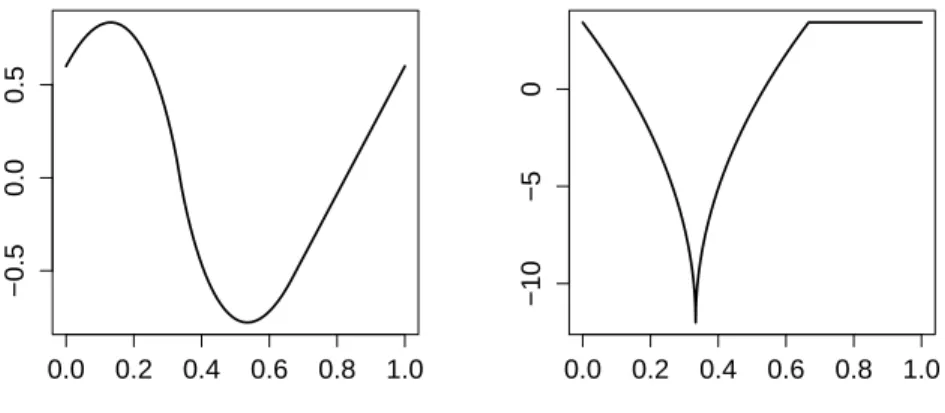
For the drift function, we first choose the function b(x) = 12(a(x) + 0.05) where
a(x) =
(
2
7 −x−
2
7(1−3x)
p
|1−3x| x∈[0,2/3)
−2
7 +
2
7x x∈[2/3,1]
0.0 0.2 0.4 0.6 0.8 1.0
−0.5
0.0
0.5
0.0 0.2 0.4 0.6 0.8 1.0
−10
−5
0
Figure 1: Left: drift function. Right: derivative of drift function
This function is H¨older-continuous of order 1.5 on [0,1]. A plot of b and its derivative is
shown in Figure 1. Clearly, the derivative is not differentiable in 0, 1/3 and 2/3.
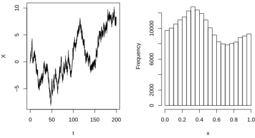
We simulated a diffusion on the time interval [0,200] using the Euler discretization
scheme with time discretization step equal to 10−5. Next, we retained all observations at
values t = i∆ with ∆ = 0.001 and i = 0, . . . ,200.000. The data are shown in Figure 2.
From the histogram we can see that the process spends most time near x = 1/3, so we
expect estimates for the drift to be best in this region. For now, we consider the data as essentially continuous time data, so no data-augmentation scheme is employed.
We define a prior with Fourier basis functions as described in Section 2.2.1, choosing
regularity β = 1.5. With this choice, the regularity of the prior matches that of the true
drift function.
For the reversible jump algorithm there are a few tuning parameters. For the model
generating chain, we chooseq(j |j) = 1/2,q(j+ 1|j) = q(j−1|j) = 1/4. For the priors
on the models we chose C = −log(0.95) which means that p(j) ∝ (0.95)mj expressing
weak prior belief in a course (low) level model. For the inverse Gamma prior on the scale
we take the hyper parameters a=b = 5/2.
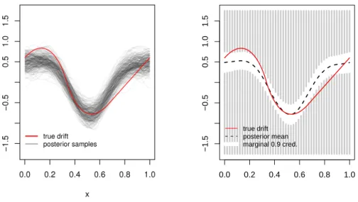
We ran the continuous time algorithm for 3000 cycles and discarded the first 500 it-erations as burn-in. We fix this number of itit-erations and burn-in for all other MCMC
simulations. In Figure 3 we show the resulting posterior mean (dashed curve) and 90%
pointwise credible intervals (visualized by the gray bars). The posterior mean was
esti-mated using Rao-Blackwellization (Robert (2007), section 4.2). (Specifically, the posterior
mean drift was not computed as the pointwise average of the drift functions b sampled at
each iteration. Rather, the average of the posterior means (Wj0)−1µj0 obtained at each
MCMC iteration (see move II) was used.)
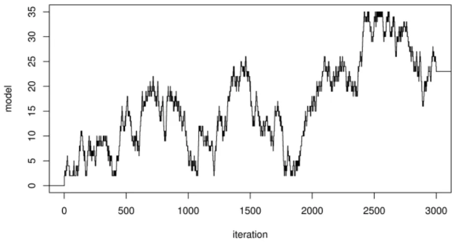
Insight in the mixing properties of the Markov chain is gained by considering traces of
0 50 100 150 200
−5
0
5
10
t
X
x
Frequency
0.0 0.2 0.4 0.6 0.8 1.0
0
2000
6000
10000
Figure 2: Left: simulated data. Right: histogram of simulated data modulo 1.
indicate that indeed the first 200-300 iterations should be discarded. Plots of the visited
models over time and the corresponding acceptance probabilities are shown in figures 5
and 6 respectively. The mean and median of the scaling parameter s2 are given by 1.91
and 1.64 respectively (computing upon first removing burn-in samples).
To judge the algorithm with respect to the sensitivity of C, we ran the same algorithm
as well for C = 0. The latter choice is often made and reflects equals prior belief on all
models under consideration. If C = 0, then the chain spends more time in higher models.
However, the posterior mean and pointwise credible bands are practically equal to the case
C =−log(0.95).
To get a feeling for the sensitivity of the results on the choice of the hyper-parameters
a and b, the analysis was redone for a=b = 5. The resulting posterior mean and credible
bands turned out to be indistinguishable from the case a=b = 2.5.
Clearly, if we would have chosen an example with less data, then the influence of the priors would be more strongly pronounced in the results.
4.1. Effect of the prior on the model index
If, as in the example thus far, the parameterβ is chosen to match the regularity of the
true drift, one would expect that using a prior where the truncation point for in the series expansion of the drift is fixed at a high enough level, one would get results comparable to
those we obtained in Figure3. If we fix the level atj = 30, this indeed turns out to be the
0.0 0.2 0.4 0.6 0.8 1.0
−1.5
−0.5
0.5
1.0
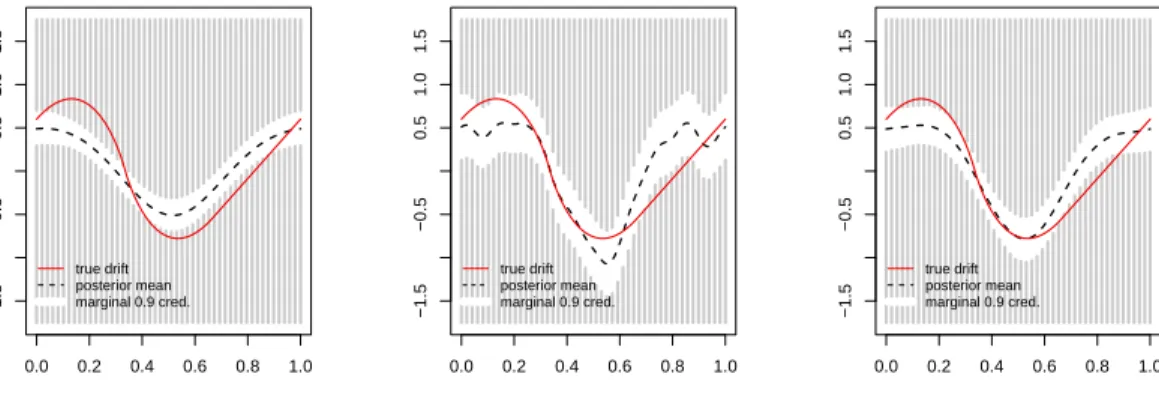
1.5
true drift posterior mean marginal 0.9 cred.
Figure 3: Left: true drift function (red, solid) and samples from the posterior distribution. Right: drift function (red, solid), posterior mean (black, dashed) and 90% pointwise credible bands
Figure 5: Models visited over time.
5 10 15 20 25 30 35
5
10
15
20
25
30
35
from model
to model
0.2 0.4 0.6 0.8 1.0
0.0 0.2 0.4 0.6 0.8 1.0
−1.5
−0.5
0.5
1.0
1.5
true drift posterior mean marginal 0.9 cred.
0.0 0.2 0.4 0.6 0.8 1.0
−1.5
−0.5
0.5
1.0
1.5
true drift posterior mean marginal 0.9 cred.
0.0 0.2 0.4 0.6 0.8 1.0
−1.5
−0.5
0.5
1.0
1.5
true drift posterior mean marginal 0.9 cred.
Figure 7: Drift function (red, solid), posterior mean (black, dashed) and 90% pointwise credible bands. Left: s2= 0.25 fixed. Middle: s2= 50 fixed. Right: random scaling parameter (Inverse gamma prior with a=b= 2.5).
For the reversible jump run, the average of the (non-burn-in) samples of the model index
j equals 18.
4.2. Effect of the random scaling parameter
To assess the effect of including a prior on the multiplicative scaling parameter, we ran
the same simulation as before, though keeping s2 fixed to either 0.25 (too small) or 50 (too
large). For both cases, the posterior mean, along with 90% pointwise credible bounds, is
depicted in Figure 7. For ease of comparison, we added the right-hand-figure of Figure
3. Clearly, fixing s2 = 0.25 results in oversmoothing. For s2 = 50, the credible bands
are somewhat wider and suggest more fluctuations in the drift function than are actually present.
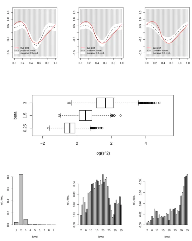
4.3. Effect of misspecifying smoothness of the prior
If we consider the prior without truncation, then the smoothness of the prior is es-sentially governed by the decay of the variances on the coefficients. This decay is
deter-mined by the value of β. Here, we investigate the effect of misspecifying β. We consider
β ∈ {0.25,1.5,3}. In Figure 8one can assess the difference in posterior mean, scaling
pa-rameter and models visited for these three values of β. Naturally, ifβ is too large, higher
level models and relatively large values for s2 are chosen to make up for the overly fast
decay on the variances of the coefficients. Note that the boxplots are for log(s2), nots2.
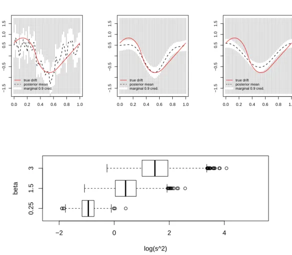
It is interesting to investigate what happens if the same analysis is done without the reversible jump algorithm, thus fixing a high level truncation point. The results are in
Figure9. From this figure, it is apparent that if β is too small the posterior mean is very
wiggly. At the other extreme, if β is too large, we are oversmoothing and the true drift
in very bad estimates if a high level is fixed. From the boxplots in Figures 8 and 9 one
can see that the larger β, the larger the scaling parameter. Intuitively, this makes sense.
Moreover, in case we employ a reversible jump algorithm, a too small (large) value for β
is compensated for by low (high) level models.
4.4. Results with Schauder basis
The complete analysis has also been done for the Schauder basis. Here we take q(j |
j) = 0.9, q(j + 1 | j) = q(j−1 | j) = 0.1. The conclusions are as before. For the main
example, the computing time with the Schauder basis was approximately 15% of that for the Fourier basis.
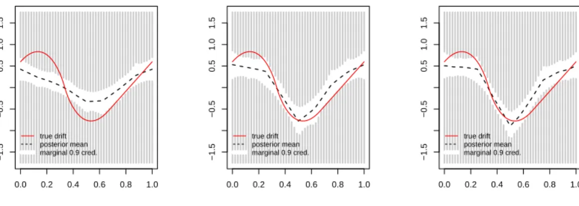
4.5. Discrete-time data and data-augmentation
Here, we thin the “continuous”-time data to discrete-time data by retaining every 50th
observation from the continuous-time data. The remaining data are hence at timest=i∆
with ∆ = 0.05 and i = 0, . . . ,4000. Next, we use our algorithm both with and without
data-augmentation. Here, we used the Schauder basis to reduce computing time. The
results are depicted in Figure 10.
The leftmost plot clearly illustrates that the discrete-time data with ∆ = 0.5 cannot be
treated as continuous-time data. The bias is quite apparent. Comparing the middle and the rightmost plot shows that data-augmentation works very well in this example.
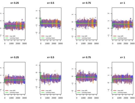
We also looked at the effect of varying T (observation time horizon) and ∆ (time
in between discrete time observations). In all plots of Figure 11 we used the Schauder
basis with β = 1.5 and data augmentation with 49 extra imputed points in between two
observations. In the upper plots of Figure 11we varied the observation time horizon while
keeping ∆ = 0.1 fixed. In the lower plots of Figure 11we fixed T = 500 and varied ∆. As
expected, we see that the size of the credible bands decreases as the amount of information in the data grows.
Lastly, Figure 12 illustrates the influence of increasing the number of augmented
ob-servations on the mixing of the chain. Here we took ∆ = 0.2 and T = 500 and compare
trace plots for two different choices of the number of augmented data points, in one case 25 data points per observation and in the second case 100 data points per observations. The mixing does not seem to deteriorate with a higher number of augmented observations.
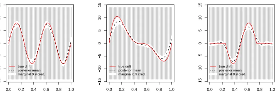
4.6. Performance of the method for various drift functions
In this section we investigate how different features of the drift function influence the results of our method. The drift functions chosen for the comparison are
1. b1(x) = 8 sin(4πx),
2. b2(x) = 200xe(1−2xe)
31
[0,12)(xe)−
400
3 (1−ex)(2xe−1)
31
[12,1)(ex), where ex=x mod 1,
3. b3(x) = −8 sin(π(4x−1))1[1
4,
3
0.0 0.2 0.4 0.6 0.8 1.0
−1.5
−0.5
0.5
1.0
1.5
true drift posterior mean marginal 0.9 cred.
0.0 0.2 0.4 0.6 0.8 1.0
−1.5
−0.5
0.5
1.0
1.5
true drift posterior mean marginal 0.9 cred.
0.0 0.2 0.4 0.6 0.8 1.0
−1.5
−0.5
0.5
1.0
1.5
true drift posterior mean marginal 0.9 cred.
● ● ●● ● ●●●●● ● ●●●●● ●●● ●●● ●●● ● ●●●● ●
●●●
●● ●●●●●● ●
● ●●● ●●●●●●● ●● ●●● ●●● ●●●●●●●●●● ●● ●●● ●●●● ● ●
● ●●●●●●●●●● ●●●●●●●●●●● ●●●●●●●● ●
0.25
1.5
3
−2 0 2 4
log(s^2)
beta
1 2 3 4 5 6 7 8 9
level
rel. freq.
0.0
0.2
0.4
0.6
0.8
2 6 10 15 20 25 30 35
level
rel. freq.
0.00
0.01
0.02
0.03
0.04
2 6 10 15 20 25 30 35
level
rel. freq.
0.00
0.02
0.04
0.06
0.08
Figure 8: Reversible jump; from left to right β = 0.25, β = 1.5 and β = 3. Upper figures: posterior mean and 90% pointwise credible bands. Middle figure: boxplots of log(s2). Lower figures: histogram of
0.0 0.2 0.4 0.6 0.8 1.0
−1.5
−0.5
0.5
1.0
1.5
true drift posterior mean marginal 0.9 cred.
0.0 0.2 0.4 0.6 0.8 1.0
−1.5
−0.5
0.5
1.0
1.5
true drift posterior mean marginal 0.9 cred.
0.0 0.2 0.4 0.6 0.8 1.0
−1.5
−0.5
0.5
1.0
1.5
true drift posterior mean marginal 0.9 cred.
●
●● ●
●● ● ●
●● ● ●● ● ●●●●●●●● ●
● ●● ●●●●● ●●●●●●●●● ● ●●●●● ●
0.25
1.5
3
−2 0 2 4
log(s^2)
beta
0.0 0.2 0.4 0.6 0.8 1.0
−1.5
−0.5
0.5
1.0
1.5
true drift posterior mean marginal 0.9 cred.
0.0 0.2 0.4 0.6 0.8 1.0
−1.5
−0.5
0.5
1.0
1.5
true drift posterior mean marginal 0.9 cred.
0.0 0.2 0.4 0.6 0.8 1.0
−1.5
−0.5
0.5
1.0
1.5
true drift posterior mean marginal 0.9 cred.
Figure 10: Drift function (red, solid), posterior mean (black, dashed) and 90% pointwise credible bands. Discrete-time data. Left: without data-augmentation. Middle: with data-augmentation. Right: continuous-time data.
0.0 0.2 0.4 0.6 0.8 1.0
−1.5
−0.5
0.5
1.0
1.5
true drift posterior mean marginal 0.9 cred.
0.0 0.2 0.4 0.6 0.8 1.0
−1.5
−0.5
0.5
1.0
1.5
true drift posterior mean marginal 0.9 cred.
0.0 0.2 0.4 0.6 0.8 1.0
−1.5
−0.5
0.5
1.0
1.5
true drift posterior mean marginal 0.9 cred.
0.0 0.2 0.4 0.6 0.8 1.0
−1.5
−0.5
0.5
1.0
1.5
true drift posterior mean marginal 0.9 cred.
0.0 0.2 0.4 0.6 0.8 1.0
−1.5
−0.5
0.5
1.0
1.5
true drift posterior mean marginal 0.9 cred.
0.0 0.2 0.4 0.6 0.8 1.0
−1.5
−0.5
0.5
1.0
1.5
true drift posterior mean marginal 0.9 cred.