ON LEARNING COMPOSABLE AND DECOMPOSABLE GENERATIVE MODELS USING PRIOR INFORMATION
Yeu-Chern Harn
A dissertation submitted to the faculty of the University of North Carolina at Chapel Hill in partial fulfillment of the requirements for the degree of Doctor of Philosophy in the Department of Computer Science.
Chapel Hill 2019
ABSTRACT
Yeu-Chern Harn: On Learning Composable and Decomposable Generative Models Using Prior Information (Under the direction of Vladimir Jojic)
Within the field of machining learning, supervised learning has gained much success recently, and the research focus moves towards unsupervised learning. A generative model is a powerful way of unsupervised learning that models data distribution. Deep generative models like generative adversarial networks (GANs), can generate high-quality samples for various applications. However, these generative models are not easy to understand. While it is easy to generate samples from these models, the breadth of the samples that can be generated is difficult to ascertain. Further, most existing models are trained from scratch and do not take advantage of the compositional nature of the data.
To address these deficiencies, I propose a composition and decomposition framework for generative models. This framework includes three types of components: part generators, composition operation, and decomposition operation. In the framework, a generative model could have multiple part generators that generate different parts of a sample independently. What a part generator should generate is explicitly defined by users. This explicit ”division of responsibility” provides more modularity to the whole system. Similar to software design, this modular modeling makes each module (part generators) more reusable and allows users to build increasingly complex generative models from simpler ones. The composition operation composes the parts from the part generators into a whole sample, whereas the decomposition operation is an inversed operation of composition.
On the other hand, given the composed data, components of the framework are not necessarily identifiable. Inspired by other signal decomposition methods, we incorporate prior information to the model to solve this problem. We show that we can identify all of the components by incorporating prior information about one or more of the components. Furthermore, we show both theoretically and experimentally how much prior information is needed to identify the components of the model.
ACKNOWLEDGMENTS
First of all, I want to thank my advisor, Vladimir Jojic, for always providing helpful advice and support. He is willing to share his excellent research idea with me. When I encountered problems in my research projects, he worked with me patiently to solve the problems. Moreover, he gave comments on my academic writings and presentations so I can improve my writing and presenting skills. When I lacked the motivation to graduate, he is the person who continually reminds me to move on. I also want to thank my committee members, Leonard Mcmillan, Marc Niethammer, Nebojsa Jojic, Ron Alterovitz, for supporting my research and giving me feedback on my works. Without them, the quality of my thesis could be much lower.
Secondly, I want to thank my senior labmate: Tianxiang Gao. When I was a new graduate student, Tianxang shared his experience with machine learning and bioinformatics so I could catch up in these two areas quickly. Moreover, I want to thank all my project collaborators: Elizabeth Shank, Matthew Powers, Zhenghao Chen. By working with them, I learn how other great people approach challenging problems. I had excellent experience in collaboration with them.
Thirdly, I want to thank all UNC-CS faculty members that are helpful for my graduation. Faculties and staffs in UNC-CS are all very lovely and very helpful. Specifically, I want to thank my former and current student service manager, Jodie and Denise. They are enthusiastic about helping me with various documents for graduation. I also want to thank Leonard Mcmillan for giving me good advice and help proceed with my graduation procedure.
TABLE OF CONTENTS
LIST OF TABLES . . . ix
LIST OF FIGURES . . . x
1 INTRODUCTION . . . 1
1.1 Generative Model . . . 1
1.2 Matrix-assisted Laser Desorption/Ionization Imaging Mass Spectrometry (MALDI-IMS) . . . . 1
1.3 Signal Decomposition . . . 2
1.4 Generative Adversarial Networks (GANs) . . . 3
1.5 Motivation from Signal Decomposition Methods . . . 4
1.6 Thesis Statement . . . 4
1.7 Limitations of Previous Signal Decomposition Methods . . . 5
1.8 Limitations of Previous GANs . . . 6
1.9 Comparisons to Related Frameworks for GANs . . . 7
1.10 Contributions and Organization . . . 7
2 BACKGROUND . . . 9
2.1 Sparse Dictionary Learning (SDL) . . . 9
2.1.1 Introduction . . . 9
2.1.2 Mathematical Notations . . . 9
2.1.3 Mathematical Formulation . . . 10
2.1.4 Training of SDL . . . 10
2.2 Generative Adversarial Networks (GANs) . . . 11
2.2.2 The Network Architectures in GANs . . . 13
2.2.3 GAN Mathmatical Formulation . . . 14
2.2.4 WGAN-GP . . . 14
2.2.5 Training of GANs . . . 16
2.3 Other Deep Neural Networks . . . 16
2.3.1 Classifier Network . . . 16
2.3.2 Encoder-Decoder Network and U-Net . . . 17
2.4 Evaluations of Models . . . 18
3 Learning Part Generators with Sparse Dictionary Learning (SDL) . . . 20
3.1 MALDI-IMS Data and a Preprocessing method . . . 20
3.2 Applying Our Framework to SDL . . . 22
3.3 Including Prior information . . . 23
3.4 Training Algorithm of the Generative Model (MOLDL) . . . 25
3.5 Biconvexity of MOLDL . . . 28
3.6 Experimental Results . . . 28
3.6.1 Synthetic Data Results . . . 28
3.6.2 Real Data Results. . . 31
4 Composition and Decomposition of GANs . . . 34
4.1 Motivation . . . 34
4.2 Compositional/Decompositional Framework of GANs . . . 34
4.2.1 Application: Image with Foreground Object(s) on a Background . . . 35
4.3 Loss Functions . . . 35
4.4 Network architecture and Training Algorithm . . . 37
4.5 Different Tasks with Different Prior Information Given . . . 38
4.6 Experiment Results. . . 38
4.6.1 Datasets . . . 38
4.6.3 Experiments on MNIST-MB . . . 39
4.6.4 Chain Learning - Experiments on MNIST-BB . . . 43
4.6.5 Transfer Learning - Experiments on Fashion-MNIST-MB . . . 44
4.7 Identifiability Results . . . 46
4.8 Identifiability proofs . . . 47
5 SUMMARY, DISCUSSION AND FUTURE WORK . . . 51
5.1 Summary . . . 51
5.2 Discussion . . . 52
5.3 Future Work . . . 54
LIST OF TABLES
1.1 Various GAN frameworks can learn some, but not all, components of our frame-work. These components may exist implicitly in each of the models, but their
extraction is non-trivial. . . 7
3.1 The possible ion products a molecule with molecular weight M could generate, under different experimental settings: positive mode and negative mode. Each row represents a type of signal coming from an ion product, named by ”Ionization
types.” The field ”m/z” is the measurement of the corresponded signal. . . 23
4.1 Table for all losses . . . 37 4.2 We show Frechet inception distance (FID)(Heusel et al., 2017) for generators
trained using different datasets and methods. The ”Foreground” column and ”Foreground+background” column reflect the performance of trained generators on generating corresponding images. WGAN-GP is trained on the foreground and the composed images directly. Generators evaluated in the ”By decomposition” row are obtained as described in Task 3 - on composed images, given background generator and composition operator. The information processing inequality (Cover and Thomas, 2012) guarantees that the resulting generator cannot beat the WGAN-GP on clean foreground data. However, the composed images are better modeled using the learned foreground generator and known composition and background
LIST OF FIGURES
1.1 Interaction between two baceria colonies (Bacillus subtilis PY79 and Streptomyces coelicolor A3) over time (Yang et al., 2012). Column one are the photos of the specimen. Column two, three, and four represent different ion fragments and their distributions in this sample. The color gradient is from least-intense ion (purple) to
most-intense ions (red). . . 2 1.2 An image example of signal decomposition. We use FastICA (Hyv¨arinen and Oja,
2000) implemented by scikit-learn (Pedregosa et al., 2011) to separate the mixed
signals. Note the separated signals only approximate the source signals. . . 3
2.1 Illustrations of the encoder-decoder network and U-net. Each arrow represents an operation (eitherCONVorTCONV), while each dotted arrow represents an addi-tional connection that copies the featrues from layer i to layer n-i and concatenates them together. C(k)stands forCONV(k, 5, 2)andTC(k)forTCONV(k, 5, 2).
Figure credit: (Isola et al., 2017) . . . 18
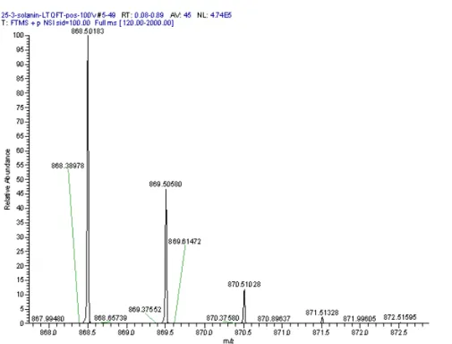
3.1 An example of a peak from low-resolution mass spectrometry. RP stands for resolu-tion power. The figure is adopted from
https://fiehnlab.ucdavis.edu/projects/seven-golden-rules/mass-resolution . . . 21 3.2 An example of peaks from high-resolution mass spectrometry. The figure is
adopted from https://fiehnlab.ucdavis.edu/projects/seven-golden-rules/mass-resolution . . . 22 3.3 A dictionary with non-zero patterns is constructed from the table 3.1. Each column
is a part generator modeling the measurements of each molecule. Each of the M1, M2, and Mn stands for a molecule’s weight. The shaded entries are the non-zero entries. Given the experiment setting (here is the positive mode) and molecular weights, we can construct the pattern for each column. Note that it is possible that two molecules share the same measurement. In this example, M1+Na and
M2+NH4have the same m/z measurement. Signal decomposition is useful for this case. . . 24 3.4 The illustrations of the tensorW andY. We arrange the samples in a 2d plate,
and each sample in the plate contains d measurements (Mass-spec imaging data). On the other hand,W models the abundances of the molecules in the dictionary D. Each sample has a corresponded abundance vector. Gaussian priors on the
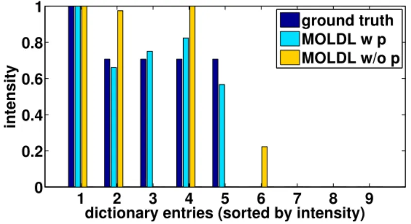
abundance differences between neighboring samples are included in our model. . . 25 3.5 The entry-by-entry comparison of the ground truth dictionary with MOLDL with
the non-zero pattern (MOLDL w p), and without the pattern (MOLDL w/o p). The entries are sorted in the descending order of the intensity in the ground truth
dictionary. The ground-truth value for each entry is1,0.707,0.707,0.707,0.707,0,0,0,0. . . . 29 3.6 The entry-by-entry comparison of the ground truth dictionary with the dictionary
from MOLDL, NNMF, and pLSA. The entries are sorted in the descending order
3.7 The distribution of the cosine similarities of the true dictionary elements and false dictionary elements for each pair of methods comparison. (A) ground truth dictionary compared to itself. (B) The dictionary from sparse-pLSA compared to the ground truth dictionary. (C) The dictionary from sparse-NNMF compared to the ground truth dictionary. (D) The dictionary from MOLDL compared to the
ground truth dictionary. . . 31 3.8 The surfactin-C14 and surfaction-C15 dictionary element from the ground truth
(purified surfactin), MOLDL, s-pLSA (sparse pLSA), and s-NNMF (sparse NNMF) in the negative and positve mode data. The negative and positive mode are exper-imental settings that are useful to capture certain types of molecules. The bars from left to right for each m/z are the intensities of that m/z in each dictionary elements. The m/z values in the brackets are the true positive m/z in the ground
truth dictionary element (purified surfactin). . . 33
4.1 An example of composition and decomposition for the application on images . . . 35 4.2 Examples of MNIST-MB dataset. 5x5 grid on the left shows examples of MNIST
digits (first part), middle grid shows examples of monochromatic backgrounds
(second part), grid on the right shows examples of composite images. . . 39 4.3 Examples of MNIST-BB dataset. 5x5 grid on the left shows examples of MNIST
digits (first part), middle grid shows examples of monochromatic backgrounds with shifted, rotated, and scaled boxes (second part), grid on the right shows examples
of composite images with digits transformed to fit into appropriate box. . . 39 4.4 Examples of fashion-MNIST-MB dataset. 5x5 grid on the left shows examples of
fasion-MNIST item (first part), middle grid shows examples of monochromatic
backgrounds (second part), grid on the right shows examples of composite images. . . 39 4.5 Given component generators and composite data, decomposition can be learned. . . 40 4.6 Training composition and decomposition jointly can lead to “incorrect”
decom-positions that still satisfy cyclic consistency. Results from the composition and decomposition network. We note that decomposition network produces inverted background (compare decomposed backgrounds to original), and composition network inverts input backgrounds during composition (see backgrounds in re-composed image). Consequently decomposition and composition perform inverse
operations, but do not correspond to the way the data was generated. . . 41 4.7 Given one part distribution, decomposition function and the other part distribution
can be learned. . . 41 4.8 Knowing the composition function is not sufficient to learn components and
de-composition. Instead, the model tends to learn a “trivial” decomposition whereby
4.9 Some results of chain learning on MNIST-BB. First we learn a background genera-tor given foreground generagenera-tor for “1” and composition network, and later we learn the foreground generator for digit “2” given background generator and composition
network. . . 44 4.10 For fasion-MNIST-MB dataset, given one part data distribution and composition
function, decomposition function and the other part generators can be learned. . . 45 4.11 Some results of chain learning on MNIST to Fashion-MNIST. First we learn a
background generator given foreground generator for digit ”1” and composition net-work, and later we learn the foreground generator for T-shirts given the background
generator. . . 45 4.12 Given one part data distribution and composition function from MNIST-MB,
decomposition function and the other part generator can be learned for
CHAPTER 1: INTRODUCTION
1.1 Generative Model
Given an observable variableXand a target variableY, a generative model is a statistical model of probabilityp(X, Y)(Ng and Jordan, 2002). Informally speaking, a generative model assigns a probability for a sample. One benefit of this modeling is it allows including prior knowledge and explicit claims about how data is generated. Therefore, our framework that has assumptions about data generation and including prior knowledge naturally builds on the generative model.
1.2 Matrix-assisted Laser Desorption/Ionization Imaging Mass Spectrometry (MALDI-IMS)
In this dissertation, I applied my framework on common data types (2d images), but also on a specific type of data generated by Matrix-assisted Laser Desorption/Ionization Imaging Mass Spectrometry (MALDI-IMS) (McDonnell and Heeren, 2007). MALDI-IMS is a technique used in mass spectrometry, that is an analytical technique to measure the masses within a sample. From these masses, we can infer the possible molecules within the sample. Precisely, with MALDI-IMS we do not measure the masses directly; instead, we measure the masses of ion fragments ablated from the molecules. Each molecule may contribute to multiple ion fragments’ measurements, and different molecules may produce ions of the same mass and charge, all contributing to the same measurement. Therefore, it is not trivial to uncover the molecules within a sample from MALDI-IMS data directly. Signal decompositions methods have been applied to uncover the source signals (signal of each molecule) from the mixed one.
Figure 1.1: Interaction between two baceria colonies (Bacillus subtilis PY79 and Streptomyces coelicolor A3) over time (Yang et al., 2012). Column one are the photos of the specimen. Column two, three, and four represent different ion fragments and their distributions in this sample. The color gradient is from least-intense ion (purple) to most-intense ions (red).
1.3 Signal Decomposition
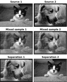
One approach to analyzing MALDI-IMS data is signal decomposition. Signal decomposition aims to separate a signal into multiple source signals. The decomposition provides a better understanding and a simpler model of input signals. Figure 1.2 is an example where two source images are decomposed (the images in the third row), given only the superpositioned-mixed images (the images in the second row) and no other information about the source images. Signal decomposition methods have been widely applied in many problems, including identification of molecules from MALDI-IMS data (Harn et al., 2015), denoising brain images (Congedo et al., 2008), decomposition of gene expressions into un-correlated groups (Ma and Dai, 2011), speech denoising (Schmidt et al., 2007), and object recognition (Koniusz et al., 2017).
Source 1 Source 2
Mixed sample 1 Mixed sample 2
Separation 1 Separation 2
Figure 1.2: An image example of signal decomposition. We use FastICA (Hyv¨arinen and Oja, 2000) implemented by scikit-learn (Pedregosa et al., 2011) to separate the mixed signals. Note the separated signals only approximate the source signals.
interpretable models for data, they are not applicable in many real use cases. For example, ICA assumes independent source signals, to which we can easily assign meanings; however, it is unsuitable to apply ICA in a foreground detection task where we want to decompose the foreground object from an image because foreground and background are not independent.
1.4 Generative Adversarial Networks (GANs)
generator and discriminator are iteratively updated until convergence. After enough training, the generator can transform a set of latent codes into a realistic sample.
GANs have many advantages, including sampling at low cost, implicitly modeling of data, and last but not the least, GANs have many successful applications including realistic face generation (Karras et al., 2017), style transfer (Zhu et al., 2017), super-resolution imaging(Ledig et al., 2017), text to image synthesis (Reed et al., 2016), text generation (Fedus et al., 2018). Due to these advantages, GANs have been gaining much attention recently. Despite great interest in GANs, trained generators are typically monolithic and difficult to interpret. One approach to understanding generators is to investigate the effects of latent codes one-by-one. This method is not scalable to a large number of codes. Other approaches to obtaining interpretable generators are to assign meaning to code from the start (Odena et al., 2016; Donahue et al., 2017), or learn disentangled codes from data (Chen et al., 2016), but there are not many ways to do this. All in all, the generators, though they are powerful, are used in the manner of a black box.
1.5 Motivation from Signal Decomposition Methods
Signal decomposition methods have their constraints (or in a milder form: regularizations) to narrow down the possible ways of decompositions. A decomposition method is suitable for a type of data if its constraints reflect the nature of data. As mentioned before, some decomposition methods with strict constraints provide easily interpretable models but usually do not reflect the data, like PCA and ICA. Decomposition methods, such as NNMF or SDL, do not have the constraints as strict as PCA or ICA. Instead; NNMF assumes input data, and source signals are non-negative, and SDL assumes input data has a sparse representation. Non-negativity and sparsity are constraints that reflect the nature of many important data types. For example, audio spectrograms are inherently non-negative, and natural images naturally have sparse representations for fixed bases (e.g., Fourier) (Wright et al., 2010). Therefore, these constraints are useful in general. Motivated by this, we propose to incorporate prior knowledge about data, from which we can construct flexible constraints for our models. Since the constraints come from data, they inherently reflect the nature of data.
1.6 Thesis Statement
parts into a sample, and an operator which decomposes a sample into parts. Dictionaries following the prior
can be learned using this formalism. Modern deep models such as GANs can also be trained and analyzed
using this formalism.
This dissertation proposes a framework for generative models. This framework aims at modeling samples that are mixtures of a set of source signals. This framework includes three components: part generators, composition operation, and decomposition operation. A model could have multiple part generators that generate different parts of a sample. What a part generator generates is explicitly defined by users. The composition operation composes the parts from the part generators into a complete sample, whereas the decomposition operation is the inverse of composition. As for the signal decomposition problem, the uniqueness of part generators may not be guaranteed. Hence, correctly identifying the part generators, composition operation, and decomposition operation is a challenge. We show that we can identify the three components by using prior information about one or more of the components. We apply this framework to a traditional signal decomposition method, dictionary learning, as well as a modern deep model, GAN. The applications show the framework helps identify the components. We also derive sufficient conditions such that the generative models under this framework are identifiable.
1.7 Limitations of Previous Signal Decomposition Methods
Our framework includes both composition and decomposition operations. In contrast, most signal decomposition methods only assume a specific composition operation and discover decomposition function as the inference of latent variable, or Maximum a posteriori (MAP) estimation of parameters. For example, in dictionary learning, a signal decomposition method, a mixture sample is modeled as a linear combination of basic elements taken as the columns of the dictionary matrixD. If also combing mixture samples in the column, we have a mixture samples matrixY, and the model for dictionary learning is:
Y =DX (1.1)
In this case,Dis given as a predefined composition operation, andX is the decomposition solution. To get the decomposition, we time the pseudo-inverse ofDon both sides of equation 1.1, and having the following:
On the other hand, probabilistic modelings of signals define the composition operation and give a way to compute the probability distributionp(Y|X, D). We can have the following to compute the decomposition distribution
p(X|Y, D) = Pp(Y|X, D)
Dp(Y|X, D)
(1.3)
As shown in equation 1.3, in a probabilistic model, one has to compute probability over all possibleX explicitly; thus, invoking the composition operation many times which is very expensive. In contrast, In my framework, decomposition is a given operation, and we can get the decomposition solution by this operation in a single pass, instead of invoking the composition operation multiple passes to infer decomposition in a probabilistic model.
Another benefit for explicitly defining the two operations is that it provides a possibility for modeling the two operators with different functions. The need for explicitly modeling the two operators happens in real cases. Consider the foreground object and background in an image for example; the composition operation is more straightforward than the decomposition operation. While the task of the composition operation is correctly putting the foreground on top of the background, the task of decomposition operation includes 1) distinguishing between the foreground and the background, and 2) inferring the complete background and foreground from its input. Under our framework, we can define a simpler model for the composition operation and a more complex model for the decomposition operation. A minor benefit for having the two operations defined separately is that we can execute each individually. In the case where we are only interested in decomposition (such as foreground detection), we do not need to execute the composition operation.
1.8 Limitations of Previous GANs
we can start to build toward ”modularity programming of GANs” by separating a complex generator into multiple simpler, independent generators. Each part generator should have an independent functionality so that it can be reused in other generative models.
1.9 Comparisons to Related Frameworks for GANs
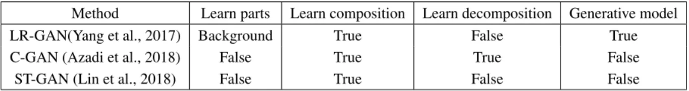
Recently the idea of composition/decomposition of GANs has been explored. LR-GAN (Yang et al., 2017) learns a composite generator that invokes each part generator recursively and learns a composition operation to stitch generated outputs together. The recursive formalism of the part generators makes the later generators depends on the earlier generators. Compared to our framework, LR-GAN learns the non-independent part generators and composition operation, but not the decomposition operation. Compositional GAN (C-GAN) (Azadi et al., 2018) learns composition and decomposition operations that have the same purposed as ours. However, C-GAN does not learn part generators, so it is not a generative model. ST-GAN (Lin et al., 2018) learns to find the correct geometric warping parameters for a foreground object, given a background and a foreground, so that the foreground and background are composed reasonably. Therefore, ST-GAN learns a composition operation but not a decomposition operation and part generators. Table 1.1 summarizes the features of each framework. Compared to others, our framework is the most comprehensive because it provides a generative model capable of learning all three components. A benefit coming from this comprehensive framework is that the composition and decomposition operations together provides a regularization for part generators. In experiments, we show we improve the quality of generators by this regularization.
Method Learn parts Learn composition Learn decomposition Generative model
LR-GAN(Yang et al., 2017) Background True False True
C-GAN (Azadi et al., 2018) False True True False
ST-GAN (Lin et al., 2018) False True False False
Table 1.1: Various GAN frameworks can learn some, but not all, components of our framework. These components may exist implicitly in each of the models, but their extraction is non-trivial.
1.10 Contributions and Organization
• Chapter 2 first presents a signal decomposition algorithm and neural network algorithms that our framework builds on. These include sparse dictionary learning, convolutional neural networks, and generative adversarial networks. Then it presents the evaluation metrics used in the dissertation. The evaluation of common signal decomposition algorithms is simple due to explicitly defined scoring function, whereas the evaluation of the algorithms of GANs is more complicated because GANs do not have such a scoring function. Consequently, we applied a GAN scoring function commonly used in the research community in this dissertation.
• Chapter 3 presents an application of our framework. Also, we include the prior information about the part generators in this algorithm so that we can correctly decompose mixed signals (decomposition operation) and recover the source signals (part generators). The experiments on synthetic datasets show this prior information is critical for recovering the correct source signals. We apply the proposed algorithm to several MALDI-IMS datasets. In these applications, we are interested in the source signals in the samples. Therefore, we evaluate the quality of the source signals resulting from the algorithm. • Chapter 4 presents another application of our framework. For purposes of exposition, we defined a family
of learning tasks in a progressively harder manner. The easier tasks have more prior information about the three components (composition operation, decomposition operation, and part generator), and the harder tasks have less prior information. We perform the experiments of these tasks on different datasets. We compare our generative model with other compositional/decompositional GANs approaches, and we evaluate the decomposition/composition operations, as well as the generative model both qualitatively and quantitatively. Last but not least, we also derive sufficient conditions such that these generative models are identifiable.
CHAPTER 2: BACKGROUND
2.1 Sparse Dictionary Learning (SDL)
In the following section, I will introduce a sparse dictionary learning method, that is used in this thesis. This introduction includes the objective, the mathematical formulation, and the training algorithm of this method.
2.1.1 Introduction
Dictionary learning is a signal decomposition algorithm that aims at finding the source signals and repre-senting the input data (mixed signals) as a linear combination of these source signals. These source signals are called dictionary elements, and together they form a dictionary. Using this dictionary, Sparse dictionary learning (SDL) further aims to find a sparse representation of the input data. This sparse representation has several advantages. First, it is easier to interpret, because most entries are zero in the representation. Second, it fits the nature of many data types, including natural images (Mairal et al., 2009) and audio (Zubair et al., 2013). Lastly, it allows learning a more flexible dictionary (e.g., dictionary elements are not required to be orthogonal) from a few high-dimensional samples (Aharon et al., 2006).
2.1.2 Mathematical Notations
Here I listed the mathematical notations that will be used later. • Bold upper case letter represents a matrix, for example,X. • Bold bold lower case letter represents a vector, for example,x. • Normal letter represents a scalar, for example,i.
2.1.3 Mathematical Formulation
Given the input dataset as a matrixX = [x1, ...,xK],xi ∈Rd, we want to find a dictionaryD∈Rd×n: D = [d1, ...,dn], and a representationW = [w1, ...,wK],wi ∈ Rnsuch that 1) the difference between
kX−DWk2
F is minimized, and 2) the representationW is sparse. This can be formulated as the following optimization problem:
arg min
D∈C,wi∈Rn K
X
i=1
kxi−Dwik22+λkwik1, whereC≡ {D∈Rd×n:kdik ≤1,∀i= 1, ..., n}, λ >0 (2.1)
In equation 2.1, the first term minimizes the difference. Since the second term is an L1-norm of the representation, it promotes the sparsity of the representation. In most cases, for large underdetermined systems of linear equation (that is the setting of SDL), the minimal L1-norm representation is also the sparsest one (Donoho, 2006). The hyperparameterλcontrols the degree of this sparsity.λis selected by an additional development dataset outside the training dataset. A constraint (C) onD is required so that its elements ([d1, ...,dn]) would not become arbitrarily large whilewiwould become arbitrarily small.
2.1.4 Training of SDL
The optimization problem that SDL aims to solve is a bi-convex problem, that is the problem becomes convex with respect to each of the variablesDandW when the other one is fixed. One training algorithm for a bi-convex problem is to trainDandW alternately. This type of algorithm is called Alternate Convex Search (ACL). In theory, ACL gives a convergent sequence of objective function and a convergent sequence of feasible solutions if its solution sets are compact (Gorski et al., 2007). In SDL,DandW are both bounded so ACL can converge to a local minimum. ACL is not guaranteed to reach the global minimum. However, ACL usually reaches good enough solutions in practice (Mairal et al., 2009).
2.2 Generative Adversarial Networks (GANs)
Since GANs are built on deep neural networks, we will first introduce the networks and their building blocks.
2.2.1 Deep Neural Networks and Layers
A deep neural network consists of an input layer, an output layer, and several hidden layers between the input layer and the output layer. Data and application determine the number of hidden layers. There are several widely-used types of layers for deep neural networks. The three types of layers most relevant to this work are a fully connected layer, convolutional layer, and transposed convolutional layer. Note that all three layers perform linear operations. In order to have a deep neural network approximates non-linear operation, an element-wise non-linear operation is usually applied after a linear layer. In this thesis, the non-linear operation refers to a rectified linear unit (ReLU), or a leaky ReLU. ReLU is the following function:
f(x) = max(0, x)
And leaky ReLU is the following function:
f(x, a) =
x ifx >0, ax otherwise,
whereais usually a small value, e.g.0.3.
A fully connected layer consists of neurons that connect all units in one layer to all units in the next layer. In a fully connect layer, the formula to compute the output for a neuronk, given theN inputs from (x1, ..., xN) previous layer, is:
ok= N
X
i=1
wixi+bk, (2.2)
A convolutional layer consists of neurons that perform convolution operation over the inputs from the previous layer. In a convolutional layer, the formula to compute the output of the neuronkat a locationiis:
oi,k = F
X
m=0
xi+m×wm,k+bk, (2.3)
wherewf,k andbk are the weight and offset for the model. Same as fully-connected layers, the number of neurons is also a hyperparameter of this layer. There are three significant differences between a fully connected layer and a convolutional layer. First, a neuron in a convolutional layer only connects toF2(filter size) inputs at a time. This restriction greatly decreases a convolutional layer’s parameter number, but still enables the neuron connects to the inputs near the target locationi. Second, the output from a neuron in a convolutional layer is not a scalar. In the above formula, the output dimension for neuronkis the same as its input. Also, an hyper-parameterS(stride) controls the output dimension. For example, a formula to compute the output of neuronkwith stride equals to two is:
oi,k = F
X
m=0
x2i+m×wm,k+bk (2.4)
With stride equals to two the output dimension is halved by two. Third, convolutional layers usually are applied to the input of 2D images, which is of two dimensions: (height, width). The two-dimensional version of the above formula is:
oi,j,k= F
X
m=0
F
X
n=0
x2i+m,2j+n×wm,n,k+bk, (2.5)
wherexi,jis a pixel in a 2D image, and every neuronkhas a weight matrix of sizeF ×F. To sum up, A convolutional layer applies convolution operation over its inputs. The hyperparameterFcontrols the number of connections to its inputs. The hyperparameterScontrols the size of the output. IfS= 1the output has the same size as the input. IfS = 2the output size is halved by two. We will use the notationCONV(k, f, s)to represent a convolutional layer withkneurons,ffilter size, andsstride.
transpose the weight matrix and multiply it by the output of the convolution operation, we will get a matrix having the same dimension as the input of the convolution operation. In the case of stride equals to two, the output of that transposed convolutional layer has size double by two. A transposed convolutional layer has same hyperparameters as a convolutional layer. We will use the notationTCONV(k, f, s)to represent a transposed convolutional layer withkneurons,f filter size, andsstride.
2.2.2 The Network Architectures in GANs
In generative adversarial networks, there are one generator and one discriminator network. They are trained against each other. While the discriminator’s goal is to correctly classify if a sample comes from real data or the generators, the generator’s goal is to increase the error rate of discriminators. Both the discriminator and the generator in GANs are deep neural networks. DCGAN (Radford et al., 2015) is a widely-used network architecture for GANs. The discriminator in DCGAN (DCGAN-disc) is a series of convolutional layers with stride of two. Since the stride equals to two, the output dimension is halved. For a 32×32image, the output dimension becomes4×4after it goes through three such convolutional layers. The neurons’ number doubles across each layer. In DCGAN-disc, when the input dimension becomes4×4, a fully-connected layer is on top of it. And the output of this fully-connected layer is a scalar indicating whether the input data is realistic, a DCGAN-disc for32×32images with one color channel has the architecture of three convolutional layers and one fully connected layer: Input data-CONV(k, 5, 2)-CONV(2k, 5, 2)-CONV(4k, 5, 2)-FC(1).
For DCGAN network architecture, the layer number of a network is fixed once the input dimension is fixed. If the input dimension is32×32, the network has three (transposed )convolutional layers. If the input dimension is64×64, the network has four such layers. On the other hand, The neuron number k is a tunable hyperparameter in DCGAN.
2.2.3 GAN Mathmatical Formulation
A generative adversarial network is a framework that estimates generative models via an adversarial process. In this process we simultaneously train two models: a generator model G that captures the data distribution, and a discriminator model D that estimates the likeliness that a sample came from the training data rather than G. Since in this adversarial process the two networks are trained against each other, training GANs is not a minimization problem but a two-player minimax game. In the original formulation of GANs (Goodfellow et al., 2014), D and G play the following minimax game :
min
G maxD V(D, G) =Ex∼pdata(x)[logD(x)]−Ez∼pz(z)[log(1−D(G(z)))] (2.6)
x∼pdata(x)represents a real sample sampling from the training set. Andz∼pz(z)represents the generated data distribution. zis a vector of codes, each drawn independently from a simple distribution, such as normal distribution or uniform distribution. The discriminatorDoutputs a probability that a sample came from the training data rather thanG.
There are many variants of GANs that use different cost functions, and there is no best GAN variant for every data and application (Lucic et al., 2018). In this work, I applied a variant called Wasserstein GAN with gradient penalty (WGAN-GP). Therefore, I will introduce WGAN-GP in details.
2.2.4 WGAN-GP
Wasserstein GAN (Arjovsky et al., 2017) is a variant of GAN trained by solving following minimax problem:
min G kDmaxkL≤1
V(D, G) =Ex∼pdata(x)[D(x)]−Ez∼pz(z)[D(G(z))] (2.7)
but a real value. Finally,Dmust be a 1-Lipschitz function. A function that has gradient smaller or equal to one is by definition 1-Lipschitz. In other words, the rate of changes of this function is bounded.
By the Kantorovich-Rubinstein duality (Villani, 2008), the Wasserstein distance between real data distribution and generated data distribution is the maximum over all the 1-Lipschitz functionsD:Rm→R (x∈Rm)
W(pdata, pz) = max
kDk≤1Ex∼pdata(x)[D(x)]−Ez∼pz(z)[D(G(z))] (2.8)
And the above equation is the objective function thatDmaximizes in equation 2.7; thus, the discriminator in Wasserstein GAN maximize the Wasserstein distance between the true and generated data distribution. And G, training adversarially againstD, minimize the Wasserstein distance.
In practice, there are several ways of makingDa 1-Lipschitz function. In this thesis, I applied a method called Wasserstein GAN with gradient penalty (WGAN-GP), (Gulrajani et al., 2017). The method includes an additional penalty term onDto regularize it to be a 1-Lipschitz function.
min
G maxD V(D, G) =Ex∼pdata(x)[D(x)]−Ez∼pz(z)[D(G(z))] +λExˆ∼pxˆ(ˆx)[(k∇ˆxD(ˆx)k2−1)
2] (2.9)
The last term in the above equation is the penalty term on the gradients ofD.λcontrols the importance of this penalty term. Usually,λcan be fixed to5, and it is robust enough for different data and applications. On the other hand, the penalty term is not put on every input domain (x) ofD. Instead, it is put only on a subset ofD’s input domain. The member of the subset is computed from the following process:
x∼pdata(x) ˜
x∼G(z),z∼pz(z) ∼U[0,1]
ˆ
x∼x+ (1−)˜x
In the original paper of the WGAN (Arjovsky et al., 2017), it shows there are several good properties of using the Wasserstein distance as a metric between two probability distrubtions. In practice, I also find WGAN-GP is more robust to different hyperparameters than the original GAN. An empirical comparison of this is shown in (Gulrajani et al., 2017). Also, the Wasserstein distance is a good indicator of the GAN training status. The generating quality has a high positive correlation with the distance. This does not happen in the original GAN formulation, where the objective function is bouncing around high and low values even in the late training iterations. Moreover, the WGAN computation does not use use logarithm and is a more straightforward computation than the original GAN.
2.2.5 Training of GANs
As training other deep neural networks, we train GANs with backpropagation algorithm. Backpropagation refers to an algorithm which uses chain rule to efficiently compute gradient of network’s output with respect to its parameters. In principle, if we can compute these gradients, we can apply any gradient descent algorithms for optimization. In this work, we apply Adam (Kingma and Ba, 2014) to optimize our model because it is has been widely used to train GANs. Adam is a type of stochastic gradient descent algorithm which only use a random batch of samples to compute the gradients. The sample size of a batch is a hyperparameter for training GANs. Also, there are two hyperparametersβ1, β2that are the forgetting factors for gradients and
second moments gradients, respectively (Kingma and Ba, 2014). These hyperparameters are either tuned with a validation dataset or set to default values suggested by the author of Adam.
2.3 Other Deep Neural Networks
2.3.1 Classifier Network
hyperparameters, including the filter size, neuron numbers, and stride are all determined by application and data. We will specify the hyperparameters of each classifier networks in the experiment section.
2.3.2 Encoder-Decoder Network and U-Net
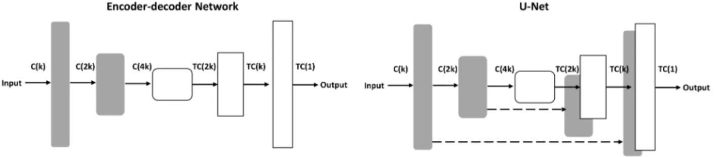
Concerning 2d image, The composition operation and decomposition operation both takes images as input and generate images as output. The two operations work similarly to the image translation in that they translate one image to another with possibly different number of channels. Encoder-decoder network architecture has been applied to solve this problem (Isola et al., 2017; Zhu et al., 2017); therefore, we also apply this network to our composition operation and decomposition operation. An encoder-decoder network is a network contains first an encoder network that extracts the high-level features from its input images, and then a decoder networks that reconstructs images from these high-level features. The encoder network contains a series of convolutional layers with stride equals to two, so it progressively down-samples its inputs and extracts complex features at this down-sampling level. The decoder network contains a series of transposed convolutional layers with stride equals to two, so the features are progressively up-sampled back to images. The encoder and decoder should have a similar number of parameters. There are no strict restrictions for this encoder-decoder network. For simplicity, we use encoder-decoder networks that have architectures similar to that of DCGAN. For example, for32×32images, our encoder-decoder network has the following architecture: Input data-CONV(k, 5, 2)-CONV(2k, 5, 2)-CONV(4k, 5, 2)-TCONV(2k, 5, 2)-TCONV(k, 5, 2)-TCONV(1, 5, 2)
Figure 2.1: Illustrations of the encoder-decoder network and U-net. Each arrow represents an operation (eitherCONVorTCONV), while each dotted arrow represents an additional connection that copies the featrues from layer i to layer n-i and concatenates them together.C(k)stands forCONV(k, 5, 2)andTC(k) forTCONV(k, 5, 2). Figure credit: (Isola et al., 2017)
2.4 Evaluations of Models
Since we have an objective function for sparse dictionary learning, we can use that function to evaluate data-fit of the model. Precisely, we optimize the function given different dictionaries on a validation dataset. For example, if we learn two dictionaries D1,D2 that come from different hyperparameter λ1, λ2, we
optimize equation 2.1 with different dictionaries (D1orD2) and compare their optimization results. Note
that when evaluating theλis fixed to zero, so we have a comparison of dictionaries with other conditions fixed. On the other hand, if we have the ground-truth dictionary of data, we can compare the learned dictionary and the ground-truth dictionary directly. If the dictionary’s dimension is small, we can show all entries of the dictionaries in a figure; otherwise, we can define a similarity index between two dictionaries so we can have a quantitative comparison. In this work, we make cosine similarity between dictionary elements as the similarity index. The details of this evaluation are shown in chapter three.
data, this metric cannot detect model collapse, a problem that a generator only generates data of low diversity compared to the real data. To cover this case, people proposed the evaluation metrics aims at computing the distance (or dissimilarity) between the two data distributions: the real data distributionPrand the generated data distributionPg. These metrics are sampling-based metrics, meaning that they rely on random draw fromPrandPg. Among all these distance computing metrics, we selected and applied the Fr´echet Inception Distance (FID) in our work because 1) it performs well compared to other metrics, and 2) Other GANs also use FID so that we can compare our results with others with fewer efforts. FID computes the follows:
F ID(Pr,Pg) =kµr−µgk+T r(Cr+Cg−2(CrCg)1/2), (2.10)
CHAPTER 3: Learning Part Generators with Sparse Dictionary Learning (SDL)
In this chapter, I show the way of applying my formalism in sparse dictionary learning and propose a novel algorithm MOLDL. The proposed algorithm MOLDL is applied to MALDI-IMS data. It is shown that MOLDL has better performance than other state-of-the-art signal decomposition methods on this type of data.
3.1 MALDI-IMS Data and a Preprocessing method
In this section, I introduce the MALDI-IMS data in details and a preprocessing method for this data. As stated in the introduction section, MALDI-IMS is an analytical technique to measure the masses within a sample plate. This technique is based on a technique called matrix-assisted laser desorption/ionization time of flight (MALDI-TOF). MALDI-TOF is an analytical technique that measures the masses within a sample. MALDI-TOF analysis is a four-step process. In the first step, the input sample is mixed with the matrix. In the next step, a pulsed laser irradiates the sample mixture, triggering desorption of the mixture. In the third step, the analyte molecules in the mixture are ionized by being protonated or deprotonated. Finally, these ionized molecules are accelerated by an electric field of known strength, and their mass-to-charge ratios are measured (Karas and Kr¨uger, 2003; Wolff and Stephens, 1953). For example, consider a molecule with a weight M is in an input sample. It is ionized as[M+H]+after the third step, and it provides a large signal of 440m/z in the fourth step. Then we can compute the weight ofM +HbyM+1H = 440, andM = 438.99 (asH= 1.01).
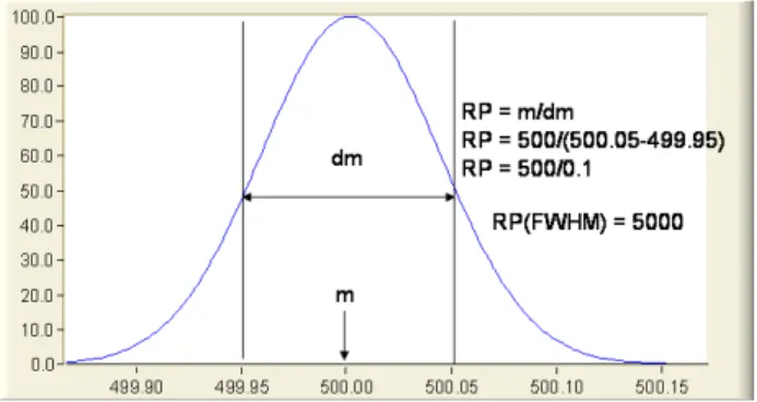
Second, a low-resolution mass spectrometry needs an algorithm to detect the ”real” m/z location. In figure 3.1, a molecule of500m/z not only has signal at that m/z but also has signals of m/zs around it. Thus, one ionization adduct generates multiple signals, but it contains only one peak at500m/z. This problem is alleviated when the spectrometry is of high-resolution (e.g. figure 3.2), but our instrument, MALDI-TOF, is not. To cope with this problem, we applied the Continuous Wavelet Transform (CWT)-based peak detection algorithm (Du et al., 2006). The main idea of this algorithm is not only considering the signal-to-noise ratio, but also the typical shape of a peak. The authors of this algorithm also showed it has the best peak-detection performance for MALDI data.
Figure 3.1: An example of a peak from low-resolution mass spectrometry. RP stands for resolution power. The figure is adopted from https://fiehnlab.ucdavis.edu/projects/seven-golden-rules/mass-resolution
Since there are still many false positive signals after the peak detection algorithm, a further reduction algorithm is needed. It is given to us that our m/z accuracy is one parts-per-million (ppm). With this information in mind, we develop a simple yet effective binning algorithm to further combining the peaks that have m/z values within the range of 1 ppm as one peak. This algorithm first sums up signals for each m/z across different samples. Since an m/z with a higher signals sum is more likely to be the center of a peak, the algorithm then bins each m/z in the descending order of signals sum we just computed. This heuristic makes binning wrong peaks less likely to happen. For an m/z m, its bin includes all the peaks in the range of [m - 0.5 ppm, m + 0.5 ppm], and the algorithm takes the maximum value in the bin to represent the value in this bin. After this step, we finish preprocessing our data. The code for the preprocessing algorithm can be found inhttps://github.com/frizfealer/IMS_project/tree/master/Bruker_ files_conversion.
Figure 3.2: An example of peaks from high-resolution mass spectrometry. The figure is adopted from https://fiehnlab.ucdavis.edu/projects/seven-golden-rules/mass-resolution
samples of MALDI-TOF with a spatial relation. We will useyi as a set of m/z signals of MALDI-TOF for a sample of index i. The number of m/z signals in each sample is determined by the preprocessing algorithm mentioned above. Consider a two-dimensional sample plate; we use two indices to represent a sample. For a sample at location i, j, we denote it asyi,j. Therefore, data for a sample plate for MALDI-IMS is a three-dimensional cube, with one dimension for m/z values, and the other two dimension for the width and the height of the plate.
3.2 Applying Our Framework to SDL
In the SDL formulation, given an input dataset as a matrixY = [y1, ...,yk],yi ∈Rd, we want to find a dictionaryD∈Rd×n:D = [d1, ...,dn], and a representationW = [w1, ...,wk], so the input matrix is best
represented. We write our dictionary learning as a generative model as follows:
This formulation is similar to the original SDL model, except the data is modeled as Poisson distributed rather than Gaussian. We assume Poisson here because our data (MALDI-IMS) is non-negative and discrete. The L1-penalty onwiin equation 2.1 corresponds to a Laplace prior onwihere.
We then apply our framework to this generative model. We regard each dictionary elementdj, j ∈
[1, ..., n]as a part generator because it should generate only a part of the data measurements. There are n such part generators. Given these part generators and the generative model, the composition and the decomposition operation are defined as a linear combination specified withwi for each samplei. The measurements of a samplei(yi) are formed by a linear combination of the measurements of the part generators.
3.3 Including Prior information
LearningDandW is undetermined if we do not provide the prior information to narrow down possible solutions. In this application, we can leverage two kinds of prior information on the part generators. The first prior information is that the measurements of the part generators have non-zero patterns.A part generator models a set of measurements generated by a specific molecule.Theoretically, a molecule only generates a few measurements in MALDI-IMS. And a molecule with a fixed experiment condition generates a fixed set of measurements. Table 3.1 shows a set of possible measurements that a molecule could generate. From the table, we can construct a sparse dictionary of these non-zero measurements (figure 3.3). Note that the non-zero entries in the dictionary are still treated as learnable parameters. If the data show no support for a non-zero entry of a part generator, the corresponding entry in that part generator will be zero.
Table 3.1: The possible ion products a molecule with molecular weight M could generate, under different experimental settings: positive mode and negative mode. Each row represents a type of signal coming from an ion product, named by ”Ionization types.” The field ”m/z” is the measurement of the corresponded signal.
(a) Postive Mode
Ionization types m/z
M+H M+1.01
M+NH4 M+18.04
M+Na M+22.99
M+K M+39.10
M+2Na-H M+44.97
M+2K-H M+77.19
(b) Negative Mode
Ionization types m/z
M-H2O-H M-19.02
M-H M-1.01
M-Na-2H M+20.98
M+Cl M+34.97
Figure 3.3: A dictionary with non-zero patterns is constructed from the table 3.1. Each column is a part generator modeling the measurements of each molecule. Each of the M1, M2, and Mn stands for a molecule’s weight. The shaded entries are the non-zero entries. Given the experiment setting (here is the positive mode) and molecular weights, we can construct the pattern for each column. Note that it is possible that two molecules share the same measurement. In this example, M1+Na and M2+NH4have the same m/z measurement. Signal decomposition is useful for this case.
The second prior information is that the signals generated from molecules should be sparse. Theoretically, a molecule only generates a few signals in MALDI-IMS. Thus, a part generator should also have a few measurements in the data. We write out this prior as a Laplace prior ondj
dj ∼Laplace(φ), j ∈[1, ..., n]
dictionary and w and h are also the width and the height (figure 3.4).We usewi,jto model the abundance of the molecules in the sample at height i and width j. In this arrangement, the nearby samples should contain similar abundances of molecules. One way to introduce this prior information to the generative model is to put Gaussian priors on the abundance differences between neighboring locations.
wi+1,j−wi,j ∼Gaussian(0, θ) wi,j+1−wi,j ∼Gaussian(0, θ)
Figure 3.4: The illustrations of the tensorW andY. We arrange the samples in a 2d plate, and each sample in the plate contains d measurements (Mass-spec imaging data). On the other hand,W models the abundances of the molecules in the dictionaryD. Each sample has a corresponded abundance vector. Gaussian priors on the abundance differences between neighboring samples are included in our model.
3.4 Training Algorithm of the Generative Model (MOLDL)
Given the generative model and the prior information, we write out the objective function as follows.
arg min
D,wi,j,λ,φ,θ;y
X
i,j
(yi,j)·log (Dwi,j)−X
i,j
{Dwi,j} (3.1)
−λX
i,j
kwi,jk1−φ
n
X
k=1 kdkk1
−θX
i,j
kwi,j−wi+1,jk22−θX i,j
In this equation, the first line corresponds to the log-likelihood function of Poisson regression. The second line corresponds to sparsity priors onD,W. The third line corresponds to Gaussian priors on the differences. We called the proposed learning problem molecular dictionary learning, abbreviated as MOLDL.
We also propose a learning algorithm to optimize this function (Harn et al., 2015). Similar to SDL, MOLDL iteratively updates dictionaryDand abundanceW until the objective function converges or the changes inW andDis smaller than a specific value.
MinimizingDwithW fixed is a non-linear optimization with two constraints. The first constraint is that the elements inDare positive. And the second constraint is that the L2-norm of each dictionary element is less than or equal to one (kdk2≤1). We applied the interior-point method to solve this optimization problem (W¨achter and Biegler, 2006). On the other hand, minimizingW withDfixed is a complex optimization problem due to its objective function. We applied the alternating direction method of multipliers (ADMM) algorithm (Boyd et al., 2011). The main idea of the ADMM is solving the problem through a divide-and-conquer approach. We divide the objective function into several sub-functions and update each sub-functions individually and alternately. We first write out the objective function as
arg min
zi,j0 ,z1i,j,z2i,j X
i,j
(yi,j)·log (zi,j0 )−X
i,j
{z0i,j} (3.2)
−λX
i,j
kz1i,jk1−θ X
i,j
kz2i,jk22
And it is subject to
z0i,j =Dwi,j, z1i,j =wi,j,
where the ”;” symbol in the definition ofz2is the row-combined operator. Then we write out this constraint
optimization as the following:
arg min
z0,z1,z2,u0,u1,u2i,j,w
X
i,j
(yi,j)·log (zi,j0 )−X
i,j
{z0i,j} (3.3)
−λX
i,j
kz1i,jk1−θX i,j
kz2i,jk22
−X
i,j
(ui,j0 )·(z0i,j−Dwi,j)−X
i,j
(ui,j1 )·(z1i,j−wi,j)
−X
i,j
(ui,j2 )·(z2i,j−[wi,j−wi+1,j;wi,j−wi,j+1])
−X
i,j ρ 2kz
i,j
0 −Dw
i,jk2 2−
X
i,j ρ 2kz
i,j
1 −w
i,jk
−X
i,j ρ 2kz
i,j
2 −[wi,j−wi+1,j;wi,j−wi,j+1]k
In this form, we can perform the ADMM algorithm, that is updating each parameter alternately. Updatingw is a linear optimization with a simple constraintw>0. Updatingz0is a non-linear optimization problem
without constraints, that can be solved by the trust-region algorithm (Byrd et al., 1987). Updatingz1 and
updatingz2 are both linear optimization problems with an L1-penalty and L2-penalty, respectively. Both of
them has a closed-form formulation for their updates. After updating all primal parameters, we update the dual parametersu0,u1,u2 with the followings:
u0 ←u0+ρ X
i,j
(z0i,j−Dwi,j)
u1 ←u1+ρ X
i,j
(z1i,j−wi,j)
u2 ←u2+ρ X
i,j
(z2i,j−[wi,j−wi+1,j;wi,j−wi,j+1])
3.5 Biconvexity of MOLDL
Biconvexity not only holds in SDL, but also in MOLDL. If MOLDL is bi-convex, it means that updating DwithW fixed is a convex optimization, and updatingW withDfixed is also a convex optimization. Theorem 3.1. The objective in equation 3.1 is bi-convex in abundances,W, and dictionary,D.
Proof. Sketch: To show that the objective function is bi-convex inW andD, we need to show that the
function is convex inW for a fixedD and vice versa. For a fixedD the objective is a sum of a convex function with an affinely transformed argumentP
i,jlog (Dwi,j), a linear functions ofw, a convex function
kwi,jk
1and another convex function with affinely transformed argumentskwi,j−wi,j+1k22. As a sum of
convex functions, the objective function is convex for a fixedD. For a fixedW, the objective function has three terms that are influenced byD. The first term is a convex function with an affinely transformed argument linear function ofD,P
i,jlogDwi,j. The second term is a linear function of D,−(
P
i,j{Dwi,j}). The third term is a convex functionkdkk1. As a sum of convex function, the objective is convex for a fixed
W. Hence, the objective is bi-convex in abundances and dictionary.
3.6 Experimental Results
3.6.1 Synthetic Data Results
We present three synthetic experiments with different purposes. We evaluate the experimental results by comparing the learned dictionary and the ground-truth dictionary. If the size of the dictionary is small, we can compare the learned dictionary to the ground truth entry-by-entry. Otherwise; we use cosine similarity to compute agreement between the pairs of dictionary elements. We compute cosine similarity for the two dictionary elementsd1,d2bycos(d1,d2) = kdd11kk·dd22k. There are two details for using cosine similarity. First,
Hungarian algorithm (Kuhn, 1955) to find the best matching of the dictionary elements. Hungarian algorithm ensures we get the best cosine similarities we could have for two given dictionaries.
The first synthetic experiment shows that the prior of non-zero patterns is useful for learning more accurate dictionaries. In the experiment, we created a ground truth dictionary that has the non-zero pattern [1,1,0; 0,1,1; 1,0,0]. and made the ground truth dictionaryDto be[0.707,0.707,0; 0,0.707,0.707; 1,0,0]. This dictionary has three dictionary elements, with the first two dictionary elements have two non-zero values, and the last dictioanry element has one non-zero value. The values ofW were generated by taking absolute values of the sample from a normal distribution(µ= 0, σ = 1). The sample size (width times height) is 20×20, andW is a tensor of size3×20×20. The result in figure 3.5 shows with the non-zero pattern (MOLDL w p), the dictionary is similar to the ground truth. Without the non-zero pattern (MOLDL w/o p), a false positive appears in entry 6, and two false negative appear in entry 3 and 5.
1 2 3 4 5 6 7 8 9 0
0.2 0.4 0.6 0.8 1
dictionary entries (sorted by intensity)
intensity
ground truth MOLDL w p MOLDL w/o p
Figure 3.5: The entry-by-entry comparison of the ground truth dictionary with MOLDL with the non-zero pattern (MOLDL w p), and without the pattern (MOLDL w/o p). The entries are sorted in the descending order of the intensity in the ground truth dictionary. The ground-truth value for each entry is 1,0.707,0.707,0.707,0.707,0,0,0,0.
elements correctly. Both NNMF and pLSA were unable to learn the correct dictionary elements in this dataset.
1 2 3 4 5 6 7 8 9
0 0.2 0.4 0.6 0.8 1
dictionary entries (sorted by intensity)
intensity
ground truth MOLDL NNMF pLSA
Figure 3.6: The entry-by-entry comparison of the ground truth dictionary with the dictionary from MOLDL, NNMF, and pLSA. The entries are sorted in the descending order of the intensity in the ground truth dictionary.
In the third synthetic experiment, we compare by the distributions of cosine similarity. The way we compute the distributions is as follows. We apply the Hungarian algorithm to find the best matching of the two dictionaries. We define the best matching as the matching having the largest overall cosine similarities. For the best matching, it containsnpairs of cosine similarities, wherenis the number of dictionary elements in the compared dictionary. Therefore, we have a distribution of cosine similarities for these pairs, and we call these ”true dictionary elements.” On the other hand, any pair is regarded as a mismatching if it is not included in the best matching. Their cosine similarities are also computed; so we obtain this distribution. We call this group of pairs ”false dictionary elements.” In figure 3.7, we compared the learned dictionary from each method (MODL, NNMF, and pLSA) to the ground truth dictionary, and we also show in figure 3.7A the comparison of the ground truth dictionary to itself as a reference. In figure 3.7A, all true dictionary elements have a cosine similarity of1, and most mismatched dictionary elements have cosine similarities closed to 0. For sparse-NNMF and sparse-pLSA,∼20%of the matched dictionary elements’ cosine similarities are around 1, and the whole distribution lies in a broad range of[0.2,1]. However, there are∼10%of the cosine similarities around0.4for both algorithms and∼10%of cosine similarities around0.2in sparse-NNMF (figure 3.7B, C). In contrast, in MOLDL, there are∼ 95%of the cosine similarities larger than0.5and
0 0.2 0.4 0.6 0.8 1 0 0.5 1 cosine similarity percentage A)
true dictionary elements false dictionary elements
0 0.2 0.4 0.6 0.8 1
0 0.5 1 cosine similarity percentage B)
true dictionary elements false dictionary elements
0 0.2 0.4 0.6 0.8 1
0 0.5 1 cosine similarity percentage C)
true dictionary elements false dictionary elements
0 0.2 0.4 0.6 0.8 1
0 0.5 1 cosine similarity percentage D)
true dictionary elements false dictionary elements
Figure 3.7: The distribution of the cosine similarities of the true dictionary elements and false dictionary elements for each pair of methods comparison. (A) ground truth dictionary compared to itself. (B) The dictionary from sparse-pLSA compared to the ground truth dictionary. (C) The dictionary from sparse-NNMF compared to the ground truth dictionary. (D) The dictionary from MOLDL compared to the ground truth dictionary.
3.6.2 Real Data Results
Our real data samples consist of two bacteria strains (Bacillus cereusandBacillus subtilits). We are interested in finding out what molecules are and how they distributed in the samples. The sample preparation includes preparing bacteria strains and media on which the strains grow.Bacillus cereusATCC14579 and
Bacillus subtilisNCIB 3610 were resuspended into Luria Broth from growth on agar plates, and resuspended to an OD600of0.5Oneµl of these cell suspensions were then spotted onto10ml agar plates (0.1X Luria
Broth, Lennox: 1g tryptone,5g yeast extract,5g NaCl and15g Bacto-agar per L). Four bacterial spots (two of each bacterial species) were put onto the agar plates in a line, with the two spots of the same species next to each other at a1cm distance, and the spots of the different bacterial species0.5cm away from each other. Colonies were grown at30°C for12or40hr before being harvested for MALDI-TOF imaging.
sample was dried overnight at37°C. Excess matrix was physically removed to clean the plate, and a peptide calibration standard was spotted onto it (Bruker part no. 206195, Pepmix4).
Here is our MALDI-IMS experiment protocol. After mass calibration using the Pepmix standard, samples were imaged using a MALDI-TOF mass spectrometer (Microflex LRF, Bruker) with a Microscout ion source (Nitrogen UV laser,λ= 337nm) in both linear positive and linear negative mode. FlexControl and FlexImaging software (Bruker) was used for image acquisition with80shots averaged from each pixel of 400to800µm across an m/z of0to5000Da.
After these experiments, we use the method mentioned before to preprocess the raw data. On the other hand, to evaluate MOLDL on the dataset, we need a ground truth dictionary to compare. From literature, we found surfactin-C13, surfactin-C14, surfactin-C15 are the molecules that should appear in our dataset. To have the ground truth dictionary elements for these molecules, we conducted MALDI-IMS experiments with purified surfactin-C13, C14, and C15. We then compare the dictionary elements learned from MOLDL with the ground truth elements. Since Surfactin-C14 and surfactin-C15 have the most complex signals and measurements, we provide the results of these molecules. The results of other molecules can be found in the supplementary of citepharn2015deconvolving. Figure 3.8a and b show the entry-by-entry comparisons of the dictionary elements from ground truth and different methods. The m/z with a bracket stands for the measurement that appears in the ground truth dictionary. Concerning these true positive measurements, the dictionary element of MOLDL has the measurements that are the most similar to the true positive measurements. Also, the dictionary element of MOLDL has the least false positive measurements. Both sparse-NNMF and sparse-pLSA have a lot of false positives, and they affect the true positives because of the shared measurements between many molecules. Including the prior information of the dictionary and abundance reduces these false positive, and result in the success of MOLDL.
0 0.2 0.4 0.6 0.8 1
m/z
intesity
399.1 399.3 399.5 400.5 1006.2 1006.7
[1021.3] 1034.4 [1057.5] ground truth
MOLDL s−NNMF s−pLSA
(a) The surfactin-C14 in the negative mode data 0 0.2 0.4 0.6 0.8 1
m/z
intesity
378.5
[1037] 1058.3 [1059.1] 1059.6 1060.2 [1075.3] [1081.1]
ground truth MOLDL s−NNMF s−pLSA
(b) The surfactin-C15 in the positive mode data
CHAPTER 4: Composition and Decomposition of GANs
4.1 Motivation
Generative Adversarial Networks (GANs) have proven to be a successful framework for training gener-ative models that can produce realistic samples across a variety of domains, including natural images and languages. However, existing GANs approaches mostly attempt to model a data distribution directly and fail to exploit the compositional nature inherent in many data distributions. Many data distributions consist of different components that are mixed through some composition process. For example, natural scenes often include various objects, composed via some combinations of translating, scaling, rotation, occlusion, etc. Our framework applying to GANs should enable it to model this compositional nature of data distributions.
4.2 Compositional/Decompositional Framework of GANs
The framework is consists of three components: part generators, a composition operation, and a decom-position operation. Here we define each component under the context of GANs.
1. Part generatorsgi(zi)A part generator is a standard generator in GANs. It maps some noise vector zsampled from a simple distribution, e.g., standard normal distribution, to a component sample. We assume there are m part generators, fromg1togm. Letoi:=gi(zi)be the output for part generator i. 2. Composition operation(c: (Rn)m →Rn)A function which composesminputs of dimensionn, that
come from the part generators to a single output (composed sample).
3. Decomposition operation(d:Rn→(Rn)m)A function which decomposes one input of dimensionn, that is a composed sample, tomoutputs (components). We denote thei-th output of the decomposition function byd(·)i. Note that the decomposition operation is the inversed operation of the composition operation.