to Sampling Error Estimation
M O N O G R A P H
National Assessment Approach
to Sampling Error Estimation
Ralph E. Folsom
This work is distributed under the terms of a Creative Commons Attribution-NonCommercial-NoDerivatives 4.0 license (CC BY-NC-ND), a copy of which is available at https://creativecommons.org/licenses/by-nc-nd /4.0/legalcode.
Library of Congress Control Number: 2014955485 ISBN 9781934831137
(refers to printed version)
RTI Press publication No. BK-0013-1412
https://doi.org/10.3768/rtipress.2014.bk.0013.1412 www.rti.org/rtipress
RTI Press RTI International
3040 East Cornwallis Road, PO Box 12194, Research Triangle Park, NC 27709-2194 USA [email protected]
www.rti.org
one or more Press editors.
Contents
Foreword v
Preface vii
About the Author viii
Chapter 1. Introduction 1
National Assessment Overview 1
Population Characteristics and Sample Statistics 2
Statistical Inference 4
Balanced Effects 9
References 12
Chapter 2. Year 01 Sampling Errors 13
Design Description 13
Parameters of Interest 14
Variance Estimators 18
Computational Considerations 26
Summary Analysis of Year 01 Sampling Errors 29
References 32
Chapter 3. Controlled Selection: Implications for Year 02 Variances 33
Introduction to Controlled Selection 33
General Population Structure and the Sample Design 34
References 43
Chapter 4. Simulation Study of Alternative Year 02 Variance Estimators 45
Simulation Model 45
Variance Approximations 54
Empirical Results 55
Comparison of Taylor Series and Jackknife Linearizations 64
References 66
Chapter 5. Comparison of Year 01 and Year 02 Sampling Errors 67
Comparative Analysis 69
References 71
Chapter 6. Conclusions 73
Appendix. Taylor Series Linearization for Regression Coefficients 75
Population Definitions 75
Estimation 76
Taylor Series Variance Approximation 76
Taylor Series Variance Estimator 80
TABLES
Table 2-1. Distribution of national design effects 29
Table 2-2. Median design effects for national P-value estimates 29 Table 2-3. Median design effects for size of community subpopulation P-value
estimates 30
Table 2-4. Median design effects for regional subpopulation P-value estimates
(9- and 13-year-olds only) 31
Table 2-5. Median design effects for sex subpopulation P-value estimates 31
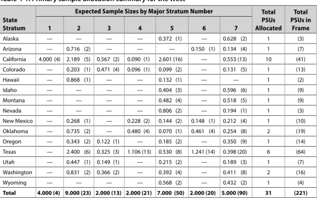
Table 4-1. Primary sample allocation summary for the West 46
Table 4-2. Bias comparisons for four variance estimators (Montreal model) 56 Table 4-3. Root mean squared error of variance estimators (Montreal model) 57 Table 4-4. Average performance of variance estimators (Montreal model) 57 Table 4-5. Sampling distributions for normal and t-like statistics 57 Table 4-6. Bias comparisons for three variance estimators under the new model
with t = 2 59
Table 4-7. Design effects with N = 744 for new model with t = 2 59
Table 4-8. Bias comparisons for the new model with t = 1 62
Table 4-9. Design effects for the new model with t = 1 (N = 744) 62 Table 4-10. Average performance of variance estimates under the new model
with t = 2 62
Table 4-11. Average performance of variance estimates under the new model
with t = 1 62
Table 4-12. Sampling distributions for Gaussian-type statistics 63 Table 4-13. Sampling distributions for Student’s t-like statistics using V2 63 Table 4-14. Bias comparisons for the new model with t = 1 and a Taylor series
linearization 64
Table 4-15. Average performance of Taylor series estimates under the new model
with t = 1 65
Table 4-16. Sampling distributions for t-like statistics 65
Table 5-1. Stem and leaf display of Year 02 national DEFFs 68
Table 5-2. Distributions of Year 01 and 02 national DEFFs 69
Table 5-3. Comparison of regional DEFFs 70
Table 5-4. Year 02 DEFFs by size of community 70
FIgURES
v
Foreword
The analysis of complex survey data is still a developing process in the 21st century. Properly taking account of complex sample design features, including stratification, multistage cluster sampling, design-based weighting, and weight adjustment processes, and applying them to both linear and nonlinear statistics have become routine
today. This was not the case when RTI International first conducted sampling and administration for the National Assessment of Educational Progress (NAEP) in 1969. In this monograph originally prepared in 1974, Dr. Folsom documents RTI’s experience in developing and evaluating appropriate sampling error estimation methods and applying them to the NAEP data.
RTI conducted the first 12 survey years of NAEP (1969–1982) under contract with the Education Commission of States (ECS) located in Denver, Colorado. The ultimate funding source for the implementation of NAEP was the federal government, but federal monitoring agencies and funding arrangements varied in the early years. ECS provided general policy guidance. Technical direction was provided by the NAEP Technical Advisory Committee (TAC), initially consisting of Robert P. Abelson, Lee J. Cronbach, Lyle V. Jones, and John W. Tukey (chair).
Each NAEP survey year included assessment of three age groups (9, 13, and 17) with samples selected from public and private school sampling frames; during the first 5 years, a sample of young adults aged 26 to 35 was also selected from an area household frame. To obtain better coverage of the 17-year-old population, out-of-school 17-year olds were also selected from the area household frame (first 5 survey years) and from special dropout follow-up samples (through 7 survey years). A form of matrix sampling was applied to cover a large battery of NAEP exercises over more than one subject with no single person required to participate for more than about an hour of assessment time. The analysis focus was on obtaining estimates for each NAEP item or exercise as opposed to an average student-level score.
help compensate for disproportionate sample numbers in five major NAEP analytic classes. For NAEP Year 02, ECS established a policy to ensure that some of the sample was selected from each state; in response to this policy, RTI implemented a controlled selection design to guarantee that each state had at least one selected primary sampling unit while preserving NAEP stratification control by region and type of community.
The complex NAEP design combined with ECS and TAC special requirements provided challenges to sampling error estimation, which Dr. Folsom addressed in this monograph. Although his focus here is primarily on NAEP Year 01 and 02 designs, the results of his work were applied to subsequent NAEP survey years. In the monograph, Dr. Folsom focused on comparing Taylor series linearization methods with the already programmed jackknife variance estimation procedures. An innovative jackknife variance estimation methodology had been developed for NAEP analysis under the guidance of John Tukey, chair of the TAC. Dr. Folsom found that the difference between Taylor series linearization and jackknife standard errors was negligible for proportions and regression coefficients when the number of strata was sufficiently large. In his subsequent Monte Carlo simulation of the NAEP Year 02 West region sample, Dr. Folsom compared the jackknife approach with the Taylor series linearization method. Although his simulation work favored the Taylor series approach, he concluded that the gains were not sufficient to justify modifying established NAEP computer programs. NAEP continues to use a jackknife variance estimation procedure.
Dr. Folsom’s work on developing Taylor series standard errors for balanced effects also extended to Taylor series estimation of sampling errors for regression coefficients and became a basis for RTI’s SUDAAN
®
software products for the analysis of complex survey and other clustered data. The current version of RTI’s SUDAAN software continues to use Taylor series approximations for nonlinear statistics but also offers users the option to use jackknife, balanced repeated replication, and bootstrap replication methods for estimating sampling error.Although many extensions have been incorporated in SUDAAN and other complex survey data analysis packages, this early work conducted by Dr. Folsom and stimulated by RTI’s first large national survey effort provides a historic perspective to the continuing evolution of complex survey analysis methods.
vii
Preface
About the Author
Chapter 1
Introduction
National Assessment Overview
The National Assessment of Educational Progress (NAEP) can be viewed as an annual series of large-scale sample surveys designed to measure the educational achievements of four age groups in 10 subject areas. The four specific age groups include all 9-year-olds and 13-year olds enrolled in school at the time of assessment and all 17-year-olds and young adults, aged 26 to 35. The first assessment of science, writing, and citizenship spanned the 1969–70 school year. Subsequent assessments were conducted during the 1970–71, 1971–72, and 1972–73 school years. This monograph was first drafted in 1974 as the Year 05 assessment of Career and Occupational Development (COD), and writing was underway and planning for the Year 06 assessment had begun. National Assessment respondents answer questions and perform tasks much the same as they would on a typical achievement test. One aspect of National Assessment that distinguishes it from the typical educational testing program is the way data are reported. Instead of calculating test scores for each respondent and forming normative distributions, analysts report results on each released exercise separately. NAEP staff hold back unreleased exercises for reassessment in subsequent years so that trend measurements will not be biased by school systems teaching to specific NAEP exercises. The reporting of separate exercises takes the form of estimated proportions responding correctly within various subgroups of the target population. Analysts use group effects that contrast the proportion of correct answers for a specific subgroup against the corresponding national proportion to detect variations in knowledge, understanding, skills, and attitudes among various segments of the population. With this method of reporting, each respondent does not need to complete the entire set of exercises. Subsets of exercises, called packages, are formed, which take approximately 50 minutes each to complete. If 10 such packages are formed for a particular age-class assessment, then 10 nonoverlapping samples, each representative of the target population, are specified and assigned a particular package.
precise statements about relevant population characteristics on the basis of fairly small samples. This monograph describes what is meant by relatively precise statements about population characteristics and shows how National Assessment sample data are being used to gauge the accuracy of reported results.
Population Characteristics and Sample Statistics
Although statisticians and other researchers familiar with survey methods are well aware of the inferential “leap” that is made when sample-based results are taken to represent population facts, many users of sample data do not readily distinguish between population parameters and sample statistics. It is the researcher’s obligation, therefore, to point out that the survey results are an imperfect approximation of the truth, an approximation whose accuracy is limited by the researcher’s financial resources and sample survey skills. The sources of error that plague survey results are numerous. Many of these error sources—such as unusable responses to vague or sensitive questions; no response from particular sample members; and errors in coding, scoring, and processing the data—are beyond the control of the sampling statistician. Nonsampling errors like these are also common to complete enumerations of a target population, such as the US Decennial Census. One advantage of a small sample survey over a complete enumeration, in addition to the obvious cost savings, is that a smaller, more highly trained, and supervised field force followed up by careful scoring and processing of the small sample data may produce fewer nonsampling errors per respondent than the large unwieldy census operation.
In addition to poor response, nonresponse, scoring, and processing errors, sample survey results are inaccurate precisely because they are based on a sample and not on the entire population. Consider, for example, the population percentage of 9-year-olds who can answer a particular science exercise correctly. For a specified sample design and selection procedure, a very large number of possible samples could be realized. Suppose that s =1,2,…S indexes the totality of possible samples that could be drawn in accordance with a specified procedure. A probability sampling method is distinguished by the fact that each sample-s has a known nonzero probability of being selected. If we denote this probability of selection by π(s) and let (s) denote the sample-s estimate for the percentage of 9-year-olds who can answer correctly, then
(1.1)
Introduction
3
sample draws with π(s) denoting the frequency of occurrence for sample-s. If this expected value does not equal the population parameter of interest, say P, then (s) is said to be a biased estimate of P. The magnitude of this bias is specified by
. (1.2)
Bias in a sample statistic may be attributed to nonsampling as well as to sampling sources; that is, statistics that would otherwise average out to the true population value can miss the mark if nonresponse, measurement, or processing errors are made. In the absence of nonsampling errors, probability samples provide for unbiased estimation of population totals like the numerators and denominators of NAEP percent correct parameters. However, strictly unbiased estimates for ratios of population totals are often unavailable. The sampling biases associated with ratio estimates are generally negligible when large-scale probability samples are involved. Some empirical evidence for this contention is presented in the simulation study (Chapter 4), where the sampling biases of NAEP percent correct estimates are discussed.
Besides the systematic errors that cause the sample estimate to miss the mark on the average, one must also recognize that it is possible to hit the target on the average while missing the bull’s eye substantially in some samples. To quantify these random sampling fluctuations, statisticians have defined the sampling variance of (s) as
. (1.3)
This quantity represents the average squared distance between the sample values and their
expectation or centroid averaged over an infinite sequence of replicated complete sample draws. A more appropriate measure of sample dispersion for a biased estimator is the mean squared error, a weighted average of squared differences between sample values and the true population value P:
. (1.4)
The mean squared error of a sample statistic has an obvious relationship to its bias and variance; namely,
The quantity most commonly used to characterize the sampling variation of a statistic is called the standard error or SE
{
(s)}
, where. (1.6)
An analogous quantity for biased statistics is
, (1.7)
often called the root mean squared error.
It is apparent from the definitions in equations 1.3 through 1.7 that the true value of these sampling error measures cannot be determined from a single sample. It is possible, however, to produce valid estimates of these quantities using the data obtained from a well-designed probability sample. Probability samples that provide for estimating the sampling variability, ordinarily the standard errors, of sample statistics have been called measurable.1 Examples of
nonmeasurable probability samples include systematic random selections from lists exhibiting periodicity and stratified random samples with a single unit selected per stratum. National Assessment is committed to designing measurable samples, samples that provide for reasonably valid estimates of standard errors. These standard errors, used in connection with respected statistical conventions, make it possible to bridge the gap between sample estimates and population facts. A statistical framework for inferring population percent correct parameters P and the associated group effects from their sample estimates is outlined in the following section.
Statistical Inference
Confidence Intervals
When one makes an inference from a sample about the magnitude of a population parameter, like P, by quoting a sample estimator (s), it is common statistical practice to include a range or interval of values about (s), which is likely to contain the true population value P. Such intervals are commonly called “confidence intervals” in the statistical literature. When the estimator is unbiased or nearly unbiased (like a ratio estimator), a confidence interval frequently takes the form
Introduction
5
where k is a constant and se
{
(s)}
is the estimated standard error for the sample statistic (s). The “confidence coefficient” associated with such an interval is the probability that a randomly selected sample will yield an interval Ip(s) that includes the true population value P. Recalling that wehave S possible samples that are realized with probabilities π(s), this confidence coefficient can be specified by defining A(P) as the set of samples where the interval Ip (s) contains P and letting
(1.9)
denote the probability that the interval associated with a randomly selected sample will contain P. Notice that the summation in equation 1.9 extends over all samples-s that belong to the set A(P)[sεA(P) denotes s belonging to A(P)]. In empirical terms, this probability statement means that, in a conceptually infinite sequence of repeated complete sample draws, a fraction γ(P) of the corresponding intervals will contain P.
To specify a value of k in equation 1.8 that will yield an interval with given confidence coefficient γ(P), one must know the sampling distribution of the standardized variable:
. (1.10)
Notice that the set A(P) of samples with Ip(s) э P [meaning the intervals Ip(s) containing P] is
equivalent to the set of samples with |t(s)| ≤ k. It is clear that the sampling distribution of t(s) cannot be specified exactly without a complete enumeration of the target population. To pursue this line of inference, sampling statisticians commonly assume that the sampling distribution of t(s) can be approximated by Student’s t distribution with “degrees of freedom” (df ). The rationale for this assumption rests on the tendency of statistics like (s) from large probability samples to have normal-like sampling distributions. With (s) approximately normal, the sampling distribution of t(s) will resemble Student’s t with the appropriate df.
For a stratified multistage sample with a total of n primary sampling units (PSUs) selected from H primary strata, the df associated with t(s) can be approximated by = (n−H). Some authors have recommended a more sophisticated approximation for df attributed to Satterthwaite.2
Satterthwaite’s approximation attempts to account for unequal within-stratum variance
A further characterization of confidence interval performance can be specified by a graph akin to the significance test power curve introduced in the next section. This confidence interval power curve summarizes the probabilities that points P* other than the true value P will not be included in the interval corresponding to a randomly selected sample. If we let α(P*)=Pr
{
Ip(s) P*}
= [1−Pr {Ip(s) э P*}], where Ip(s) has the form in equation 1.8, then
where
and
(1.11)
has the form of Student’s noncentral t statistic with df degrees of freedom and noncentrality parameter δ* = ∆*⁄se
{
(s)}
. For values of P* deviating considerably from the true value P, one would hope that Ip(s) would exclude P* with high power α(P*).It is important to note at this point that, for a given sample design and an estimation scheme characterized by se
{
(s)}
and the df associated with se{
(s)}
, the entire power curve for the confidence interval is specified once k is set. With this in mind, it is clear from equation 1.11 that although an increase in k will raise the confidence level, [γ(P) = 1−α(P)] , of the associated interval, it will also decrease the probability of excluding unwanted values. Another way of viewing this relationship between increasing confidence and the inclusion of more unwanted values (P* ≠ P) is gained by observing that the expected length of a random interval such as Ip(s)
Introduction
7
Significance Tests
When a sizeable group effect is observed in the sample, one can ask if it is likely that such an effect could be due solely to sampling variations. To answer such questions, statisticians have devised an inferential structure known as the test of significance. We describe this structure in the context of National Assessment “group effects”:
(1.12)
where G(s) denotes the sample-s estimate of the proportion of group G members who can answer
a particular exercise correctly and G(s) depicts the corresponding proportion for the entire
population. Group G could, for example, denote the 9-year-olds residing in NAEP’s Northeast region, in which case ∆ G(s) would compare the performance of the Northeast 9-year-olds against
the overall national performance of 9-year-olds.
An observed group effect ∆ G(s) is judged to be significantly different from zero if its
absolute value exceeds a critical value C. The critical value is determined so that the probability of observing an absolute effect ∆ G(s) in excess of C when the true population effect ∆ G is zero is
less than some arbitrarily small probability α. This probability α of declaring an observed sample effect significant when, in fact, the true population effect is zero is called the significance level of the test. Commonly used significance levels are α = 0.01 and α = 0.05. The critical value C frequently takes the form
, (1.13)
where k is a constant and se
{
∆ (s)}
is the estimated standard error for the group effect ∆ G(s).The subscript G designating a particular subgroup has been dropped from the group effect symbol in equation 1.13 to simplify our notation. If we let A(∆P) denote the set of samples for which ∆ (s) exceeds k se
{
∆ (s)}
in absolute value and use(1.14)
to denote the probability that an observed group effect ∆ G(s) will be judged significant, then
α(∆P) can be expressed as follows:
where
Notice that, as with the confidence interval power curve presented in equation 1.11, α(∆P) can be specified in terms of the sampling distribution of a statistic t(s, ∆P) that has the form of Student’s noncentral t statistic. If ∆P, the true population group effect, were zero, then α(0) = Pr
{
|t(s)|>k}
represents the significance level of the test with t(s) taking the form of Student’s central t statistic. For populations with ∆P ≠ 0, α(∆P) gives the probability of declaring significance when the true group effect is ∆P. Taken as a function of ∆P, the curve α(∆P) described in equation 1.15 is called the power function of the significance test. As ∆P deviates increasingly from zero, one would hope that α(∆P), the probability of declaring significance, would rise sharply.Although the power curve for our confidence interval could be completely determined if the population were fully specified, only one point of the significance test power curve can be determined: namely, that point corresponding to the true group effect ∆Po. The other points are
conceptual in the sense that they specify what the probability of declaring significance would be for a similar population where the true group effect was ∆P* ≠ ∆Po.
Prescribing a critical value for a test of significance that will yield a predetermined significance level α presumes knowledge of the sampling distribution of t(s, ∆P) = ∆P(s)/se
{
∆P(s)}
for a conceptual population, which is like the population of interest and is characterized by a negligible group effect ∆P = 0. At this point, as was the case with confidence intervals, sampling statisticians commonly assume that Student’s central t distribution would be a reasonable approximation for the sampling distribution of t(s, ∆P) from a population with ∆P = 0. When the degrees of freedom associated with se{
∆P(s, 0)}
are sufficiently large, one can effectively use the standard normal distribution to determine k such that Pr{
|t(s, 0)|>k} =
α.Various rules of thumb can be found in the literature for when the standard normal approximation is adequate, ranging from df greater than 30 to df exceeding 60.Introduction
9
in the power to declare significance when the true group effect ∆P deviates from zero. This same relationship was noted between increasing confidence coefficients and lengthening intervals.
In addition to the direct comparisons between subgroup and national proportions of correct answers, which we have called group effects, National Assessment reports adjusted or balanced effects that attempt to correct for the masking of effects due to imbalances across other characteristics. Although the unadjusted group effects properly reflect the differences in achievement between specific groups of children, much of the observed difference may well be attributable to other factors on which the compared groups differ. For example, part of the deficit in achievement observed in the direct comparison of black students with nonblacks may be attributed to the fact that black students tend, more than nonblack students, to have less educated parents. In the following section, the adjustment methodology used by National Assessment to compensate for some of this masquerading is presented.
Balanced Effects
The major population subgroupings used in National Assessment reports are age, region, size and type of community (STOC), sex, race, and parent’s education. Within the four age classes, group effects contrasting the levels of the other five factors are presented. As we have indicated, these direct comparisons across the levels of a single factor are subject to masquerading
influences of the other four factors. This confusion is partially due to the unbalanced mix of these other characteristics across the levels of any single factor being examined. To balance out this disproportionality, National Assessment forms adjusted group effects (expressed in percentages) that, when combined by addition with each other and with the overall “national” percentage of success, give fitted percentages of success ( Bal) that correspond with the actual sample data in the
following way:
If we let i taking the values 1 to 4 [i = 1(1)4] index NAEP’s four regions; j = 1 (1)7 the seven STOC categories; k = 1, 2 the two sexes; = 1(1)3 the three race classes; and m = 1(1)5 NAEP’s five levels of parent’s education, then the fitted Bal value for subclass (ijk m) has the form
, (1.16)
where is the overall (national) percentage correct and the ∆ terms represent the “balanced” group effects for region-i, STOC-j, sex-k, race- , and parent’s education class-m. With (ijk m) denoting the estimated population size for subclass (ijk m) and (ijk m) representing the estimated number of correct responses from this subclass, the balancing condition verbalized above translates into the following fitting equations:
(1.17a)
. (1.17b)
Similar sets of equations are produced for the other three classifications by summing over all the subgroups within a particular factor level and equating to the estimated total correct for that factor level. Notice that we use a plus sign to denote a summed-over subscript. Substituting the linear main effects model in equation 1.16 for B al (ijk m ), we see that the fitting equations become
and
(1.18a)
(1.18b)
Introduction
11
The other three sets of fitting equations are arrived at similarly. Notice that we have suppressed the summed-over subscripts to make the expressions more compact. Because each of the sets of fitting equations corresponding to a particular classification factor sums to the same quantity, namely,
(1.19)
one of the equations in each set is redundant. That is, of the 4 + 7 + 2 + 3 + 5 = 21 balancing equations produced in this fashion, only 16 are independent. To solve for our 21 balanced effects, we need five additional equations. Requiring that the overall in our model (equation 1.16) be equivalent to the unadjusted national P-value ( = / ) implies in equation 1.19 that
(1.20)
Setting each of these sums equal to zero yields five independent equations, which can be substituted respectively for the last equation in each of the original five sets. This substitution yields 21 independent equations, which can be solved to provide the full set of balanced effects.
Although this balancing solution was not derived with the least squares principle in mind, one can view the results as a sample estimate of the least squares solution that would be obtained if the entire population of correct-incorrect (1-0) responses were predicted by a linear model with an intercept and 21 dummy variables indicating membership in the 21 factor-level subgroups. The weighted restrictions in equation 1.20, with the “hats” removed from the population sizes (Ms), are commonly applied to unbalanced data sets. This dummy-variable regression view of NAEP’s balanced fitting places the results in a familiar statistical setting where the adjustment of regression coefficients for unbalanced representation across categories is a well-known property.
give only an indirect indication of the parents’ attitude toward education or their inclination to assist the student with homework. Another potential problem with direct comparisons between subgroups is the fact that the performance of a given subgroup may differ from one subgroup to another in the other variables. That is, the effects associated with black students may be different in the West than in the Southeast. Such interaction effects are not accounted for in NAEP’s balancing model. In spite of these deficiencies, balancing represents a big step from the outward appearances of unadjusted group effects toward the inward realities of cause and effect.
References
1. Kish L. Survey sampling. New York: John Wiley and Sons; 1965.
2. Satterthwaite FE. An approximate distribution of estimates of variance components.
Chapter 2
Year 01 Sampling Errors
Design Description
The NAEP Year 01 sample for the three in-school age classes (9, 13, and 17) began with a highly stratified, simple random selection of 208 PSUs. These primary units consisted of clusters of schools formed within selected listing units. The listing units were counties or parts of counties. Variables used to stratify these listing units were (1) region (four geographic regions), (2) SOC (four size-of-community classes), and (3) SES (two socioeconomic status categories). Within each selected listing unit, we selected a separate set of schools for each of three age groups: 9-year-olds, 13-year-olds, and 17-year-olds. For each of these age groups, we grouped schools such that every set would contain a mix of high and low SES students. Portions of some large schools were allowed to belong to more than one group. The number of schools in each of these clusters was based on the numbers of packages or questionnaires required from each PSU. The 17-year-old assessment, for example, employed 11 separate group-administered packages and 2 individually administered packages. Group administrations consisted of 12 students, while each individual package was given separately to 9 students in each PSU.
We designed the sample to yield two primary units from each of 104 strata. For the 17-year old assessment, (11 x 12) + (2 x 9) = 150 students were required from each PSU. The groups of 17-year-old schools were constructed to contain approximately 300 17-year-olds each. Once a cluster of schools was selected via simple random sampling from those constructed, we allocated the group packages to schools. Each school in the cluster was assigned a number of group administrations roughly proportional to its enrollment of 17-year-olds. Sixteen students were selected for each group session assigned to a particular school: 12 to participate and 4 to be alternates.
selected, 1 to participate and 1 alternate. This design yielded a planned sample size of 2,448 students for each group-administered package and 1,836 for each individual package.
The Year 01 out-of-school sample of young adults aged 26 to 35 and out-of-school 17-year olds used the same basic primary sample design as the in-school sample. We used the same random draw to select PSUs in both samples; however, the out-of-school PSUs were defined in terms of a set of area segments or clusters containing an average of 35 to 40 housing units. We constructed each of these PSUs to contain about 16,000 persons. The second-stage sample was a stratified random cluster sample with two clusters selected without replacement from each of five strata. The stratification was based on an ordering of segments in terms of the percentage of families earning less than $3,000. The high-poverty (low SES) quarter of the list was assigned two strata for a 2-to-1 oversampling of the low SES quarter. Each household cluster was expected to yield 12.5 eligible adult respondents. We administered 10 packages of exercises to young adults with each respondent randomly assigned a single package. Out-of-school 17-year-olds encountered in the household sample were asked to respond to a set of 4 or 5 of the 17-year-old in-school packages. Recall that there were 13 such packages. An incentive payment of $10 was given for completing the set of packages.
Parameters of Interest
Proportions Correct (P-Values)
The purpose of National Assessment (Year 01) was to produce baseline estimates of the proportions of potential respondents who would answer a certain exercise in a particular way. Restricting our attention to a particular in-school age group (say 17-year-olds) and a particular exercise within one of the packages, let
1 if the k-th sudent is school (j) of PSU (i) in =
Yhijk stratum-h answers correctly; 0 otherwise.
The population means of these 0, 1 variables are the population proportions of interest, that is
Year 01 Sampling Errors
15
where
H = the number of strata (104 planned) Nh = the number of PSUs in a stratum (h)
Shi = the number of schools in a PSU (hi)
Mhij = the number of students in a school (hij)
and
Our sample estimates for these proportions are of the form
(2.2)
where
nh = the number of PSUs selected for the sample from stratum (h) (generally nh = 2)
shi = the number of schools in PSU (hi) in which the particular package of interest was
administered
mhij = the number of students from school (hij) who respond to the package of interest and,
aside from nonresponse adjustments,
Whijk = 1/Pr {PSU (hi)} x Pr {Sch (j) | (hi)} x Pr {Kid (k) | (hij)} (2.3)
with
For group-administered packages, the number of sample schools per PSU (shi) was always 1 in Year 01. Individual packages were administered in more than one school; that is, shi ≥ 1 for
Year 01 individual package exercises.
The estimation of out-of-school, young adult, P-values parallels the procedure presented for the Year 01 in-school sample. If we let j subscript area segments instead of schools and k young adults instead of students, the expressions in equations 2.1 and 2.2 are interchangeable. To complete the switch, we let Shi denote the number of segments in the PSU-hi frame and shi
of eligible young adults in segment-hij and mhij the number of young adults in segment-hij
responding to a particular package. The out-of-school sample weights reflect the selection probabilities for young adults plus adjustments for nonresponse.
We combined out-of-school 17-year-olds located and tested in the household survey with in-school respondents to estimate a single P-value for all 17-year-olds. The total number of out-of school 17-year-olds and the number that could respond correctly were estimated for each 17-year old package using weight sums for all package respondents and for all respondents answering correctly. We then added these estimated totals to the denominator and numerator of the in-school package P-value.
Subpopulation P-Values and
∆
P Values
In addition to the national P-values discussed in the previous section, certain subpopulation breakdowns were of interest. For example, P-values have been presented by region, STOC, sex, race, and parent’s education. These subpopulation P-values were produced by including only those observations belonging to the subpopulation of interest in the numerator and denominator of equation 2.2. We studied differences between subpopulation and national P-values to assess the main effects of region, STOC, race, sex, and parent’s education. These direct comparisons were introduced as group effects or ∆P-values in the first chapter.
Balanced Effects
In the first chapter of this monograph, we introduced NAEP’s algorithm for adjusting group effects. This adjustment was designed to correct for the masquerading effect of ancillary variables when their distributions vary across the levels of the factor being examined. The adjustment or balancing algorithm used amounts to a set of linear equations that can be viewed as a sample approximation to the normal equations that would result from a least-squares fit to the population of 1-0 (correct-incorrect) responses based on an intercept and dummy variables indicating the levels of NAEP’s five reporting categories. NAEP staff imposed a set of restrictions on the balanced effects, which forced the linear model intercept to equal the observed national P-value. The left-hand sides of the balancing equations involve weighted sample estimates of population counts in the one-way and two-way margins of NAEP’s region by STOC, sex, race, and parent’s education classification. The right-hand sides of the balancing equations involve estimated counts of correct responses from the five one-way margins. Suppose we let Xhijk denote a 1 x 22 row vector for
Year 01 Sampling Errors
17
depending on the respondent’s membership in the 21 subgroups formed by NAEP’s reporting categories (4 Regions + 7 STOCs + 2 Sexes + 3 Races + 5 Parent’s Education classes). Recalling that Yhijk is 1 if the respondent (hijk) answers correctly and 0 otherwise, we can specify the balancing
equations prior to substitution with the restrictions as
(2.4)
where
and
As noted in the first chapter, the balancing equations in equation 2.4 are not linearly independent because the sum of the 2nd through the 5th equations equals the 1st as do the 6th through the 12th, the 13th and 14th, 15th through 17th, and the 18th through 22nd. To provide for a unique solution and at the same time force the intercept to equal the observed national P-value, NAEP staff replaced the final equation in each of the five blocks, which correspond to the five reporting variables, with a linear restriction on that variable’s balanced effects. For example, the fifth equation in equation 2.4 was replaced by
(2.5)
T
This substitution can be accomplished by replacing the fifth row in
(
Xhijk Xhijk)
with a (1 x 22) row vector with all elements except the second through the fifth set to zero. The four elements in columns two through five of the new fifth row take the value one or zero to indicate membershipT
in regions 1 through 4 successively. The fifth row of
(
Xhijk Yhijk)
is set to zero for every
rows 12, 14, 17, and 22 with the linear equations in equation 1.20 produce NAEP’s restricted set of balancing equations. In our further treatment of balancing,
(
XT X)
hijk and(
XT Y)
hijk representthe restricted respondent-(hijk) contributions to the left- and right-hand sides of the balancing equations. Substituting these independent linear restrictions for the redundant rows of
(
XT X)
and setting the corresponding rows of(
XT Y)
to zero allow one to specify the balanced fit uniquely aswhere
and
(2.6)
Variance Estimators
Variance Estimators for P-Values and ΔP-Values
To support the presentation of P-values and ∆P-values, we needed measures of the sampling variability of these statistics. We tailored a jackknife replication procedure for estimating the sampling variance of nonlinear statistics from complex multistage samples to our design. This technique is easily applied to highly stratified designs with only two PSUs selected with replacement or without replacement from strata where the finite population correction (nh/Nh)
can be ignored.1,2 The Year 01 primary sample fits this description except for a few strata
containing single primary units. These singleton PSUs are accounted for in the following section. To demonstrate the computational aspects of this technique, we can consider estimating the variance of a national P-value. First, we define expanded-up PSU totals
Year 01 Sampling Errors
19
and
(2.8)
Recalling equation 2.2, we see that the total hi represents the PSU-hi contribution to our sample
estimate of the number of 17-year-olds in stratum-h, while Ŷhi is the PSU-hi contribution to the
estimated number of 17-year-olds in stratum-h who could answer the question correctly. In terms of these expanded PSU totals, the P-value becomes
The jackknife estimate of , say JK, and its variance estimator are special applications of the
(2.9)
following general result for a sample of H strata with nh primary selections per strata (with
replacement or without from strata such that nh/Nh is negligible).3
Let o depict a statistic based on data from all nh PSUs in each stratum. Define the replication
estimate -hi constructed from all the PSUs excluding PSU-i in stratum-h. These replication
estimates should be produced as if this censored PSU had not responded; that is, reasonable nonresponse adjustments should be used in estimating θ without PSU (hi). The jackknife pseudo-values hi are then formed where
(2.10)
The jackknifed alternative for o is
(2.11)
A consistent estimate of the variance of JK is
where
and
Commenting on an earlier draft of this report, Dr. David R. Brillinger pointed out that a pseudo-value of the form
would be more appropriate for a stratified sample.4 This result was obtained by approximating the o
expectations of , -hi, and -h with Taylor series of the form
Using the series approximations above, one notes that
Therefore, for Brillinger’s alternative jackknife estimator
it is clear that
Year 01 Sampling Errors
21
Applying a similar argument, one can demonstrate that the jackknife estimator proposed in equation 2.11 contains first-order bias terms, namely
The variance approximation proposed for * JK by Brillinger has the form
The variance expression above is equivalent to the estimator in equation 2.12.
Applying Brillinger’s result to produce a jackknifed estimate of = o, we first consider the case where all nh = 2. If this were the case, then
(2.13)
The replicate P-values become
(2.14)
The first P-value is formed by discarding PSU 1 in stratum-h and replacing its contribution to the numerator and denominator of with the data from its companion PSU (h2). The second P-value is formed by discarding PSU 2 in stratum-h and replacing its contribution with that from PSU (h1). The jackknife pseudo-values become
(2.15)
And the jackknife P-value is
Equation 2.16 shows that the jackknife P-value is (H + 1) times the standard combined ratio
estimate minus H times the simple average of the replicate P-values. The variance estimate for
JK is
(2.17a)
Considering and recalling that Ph. = (H + 1)P – H -h., we need not bother
with the pseudo-values; that is,
(2.18a)
For nh = 2 a convenient simplification for the expression in equation 2.18a is
(2.18b)
The simplified form for the jackknife variance estimator in equation 2.17a becomes
(2.17b)
An analogous application of this technique produces ΔP-values from replicates formed by successively deleting PSUs and replacing their contributions with data from their companion PSU. If these replicate ΔP-values are denoted by Δ -hi , then the jackknife ΔP-value is ΔPJK, where
with variance estimator
(2.19)
For those unfamiliar with the jackknife linearization technique described above, it may be of interest to note the relationship between varJK ( JK) in equation 2.17 and the standard Taylor series
variance approximation for a combined ratio.5 If we let бŶh = (Ŷh1 – Ŷh2) and б h = ( h1 – h2),
the Taylor series variance approximation for var
{ }
is
Year 01 Sampling Errors
23
or
with
and
(2.20b)
Examining the form of the jackknife replicate P-values in equation 2.14, it is not difficult to see that
(2.21)
which leads to
(2.22)
Comparison of the Taylor series and jackknife variance estimators in equations 2.20 and 2.22 points out the close analytic relationship between the two. The quantity б2 h / 2 in the
denominator of the jackknife variance expression in equation 2.22 is the stratum-h contribution to the estimated relative variance of , where
(2.23)
Variance Estimators for Balanced Effects
Recalling the definitions of
(
XT X)
hijk and(
XT Y)
hijkʹ the restricted respondent-(hijk)contributions to the left- and right-hand sides of our balancing equations, we begin by forming the expanded PSU-hi totals
(2.24a)
and
(2.24b)
These definitions allow us to specify the quantities
(
XT X)
and(
XT Y)
as stratum sums of the formand
(2.25a)
(2.25b)
The jackknife replicate estimator for the vector β of balanced effects, which is obtained by deleting the contribution from PSU-h1 and replacing it with the contribution from PSU-h2, can be
specified as the unique solution to the following set of normal equations:
(2.26)
where
Year 01 Sampling Errors
25
Deleting the contribution from PSU-h2 and replacing it with the PSU-h1 contribution results in the set of normal equations:
(2.27)
which can be solved for the replicate estimate β-h2. Jackknife pseudo values
(2.28)
are then formed from the replicate estimators, where β represents the estimated vector of balanced effects based on data from all PSUs. The jackknifed estimator for β is then
(2.29)
To estimate the variance-covariance matrix of the jackknifed vector of balanced effects, we use
where
(2.30)
Notice that is a (22 x 1) column vector, and бT the transpose , is a (1 x 22) row vector.
The resulting quantity in equation 2.30 is, therefore, a (22 x 22) matrix of estimated variances and covariances among the 21 balanced effects and the corresponding national P-value, P.
In the appendix, we illustrate the derivation of the corresponding Taylor series approximation for the variance-covariance matrix of . This method yields the estimator
where
Although it is not immediately apparent, there is again a close relationship between the form of
the jackknife and Taylor series variance-covariance estimators. Subtracting matrix equation 2.27 from 2.26 and rearranging terms, one finds that
(2.32)
where
and
In solving the set of equations in equation 2.32 for бβ h , the difference between our two jackknife
pseudo values from stratum-h yields
(2.33)
Using the expression for бβ h presented in equation 2.33, shows that the jackknife
variance-covariance estimator in equation 2.30 differs from the corresponding Taylor series estimator only to the extent that β-h•, the average of our two replicate estimators from stratum-h, differs from the
estimate based on all the data. As the number of strata increases, one would expect the difference between β and β-h• to get small. For National Assessment’s Year 01 sample design with 104
primary strata, there should be little difference between the two methods.
Computational Considerations
The major complication that arose in applying the procedures introduced in the previous sections to National Assessment data was strata with only one PSU. To allow these strata to contribute to variance, we formed pseudo strata containing two or three of these singleton PSUs. This collapsing of strata was done within regions and as much as possible within SOC (size of community) superstrata. State and county names for these PSUs were also used in the matching. When two PSUs from different strata are collapsed, some adjustment should be made for the fact that the stratum sizes (Nʹhs) may be quite different. One such adjustment is to replace the stratum
Year 01 Sampling Errors
27
for a design with two PSUs selected from the union of strata-h and - ; that is, use the common expansion factor (Nh+Nℓ)/2. When applied to our jackknife methodology, this adjustment
amounts to replacing stratum- hʹs contribution to with
(2.34a)
and
(2.34b)
We “borrowed” the data from stratum-
ℓ
in terms of estimated numbers of 17-year-olds per PSU (mℓ ) and estimated numbers of correct respondents per PSU (yℓ ), but we retained the numberof PSUs appropriate for stratum-h. The contribution from stratum-ℓ is similarly replaced by stratum-h data, but its number of PSUs (Nℓ) is retained. The adjusted replicate P-values for
collapsing singleton strata-h and ℓ are, therefore,
(2.35a)
and
(2.35b)
The resulting squared difference between -ℓ and -h divided by four is a conservative estimate
(overestimate) of the variance contribution from strata-h and -ℓ. When an odd number of singleton PSUs was available within a major region, by SOC stratum, we used the last three singletons to form three pseudo strata, each comprising one of the possible pairings among the three units. The variance contribution from three singletons was estimated by adding the three squared differences divided by eight. The division by eight results from the fact that each of the three PSUs was accounted for in two of the squared differences.
An alternative stratum size adjustment, which requires no knowledge of the separate stratum sizes, Nh, uses the estimated student population from the singleton strata in the adjustment.
Assuming that the PSUs in the two collapsed strata all contain approximately the same number of students, say M, then the sum of weights for a singleton stratum-h estimates
When the h-th stratum is discarded in the replicate P-value estimation, its contribution to the numerator is replaced by its estimated population sizes
(
h)
times the estimated proportioncorrect from stratum-ℓ; that is,
(2.37)
No change is made to the denominator with this adjustment. Such an adjustment forces an equality of PSU sizes, which is not achieved for two legitimate selections from the same stratum and, therefore, would seem to underestimate the variance in this respect. As long as collapsing is not extensive, the differential effect of the two alternatives is probably negligible.
Aside from the problems surrounding stratum collapsing, applying the jackknife technique to National Assessment data was straightforward. In one pass through the data tape, sums of weights for correct responses and total sums of weights were computed within each PSU for a specified cross-classification of subpopulations. Consider for example, the cross-classification of region, STOC, sex, race, and parent’s education, yielding a five dimensional table (4 x 7 x 2 x 3 x 4), each cell of which gets a sum of weights correct Ŷhi (r, s, t, u, v) and a total sum of weights hi (rstuv)
for each PSU (hi). All of the P-values, ΔP-values, and their variance estimators can be easily computed from sums and differences of these stored quantities. The balanced effects are functions of one- and two-way marginal sums from the and Ŷ tables. The variances and covariances of the βs are formed from within-stratum PSU differences among these one- and two-way marginal totals.
Although the jackknife replication procedure was first introduced by Quenouille1 as a
technique for reducing sampling bias in nonlinear statistics, this feature is probably not of primary importance in large samples such as National Assessment, because combined-ratio type estimators like NAEP’s P-values, ΔP-values, and balanced effects should be relatively free of sampling bias. Some empirical justification for this contention can be gained by contrasting the jackknifed versions of these statistics with the original estimates. For most of NAEP’s reported statistics, these differences are negligible. For these reasons, National Assessment reports unjackknifed statistics along with the associated jackknife variance estimator.
In the following section, we present a summary analysis of Year 01 sampling errors. These results were extracted from a paper by Chromy, Moore, and Clemmer.6 The results are presented
Year 01 Sampling Errors
29
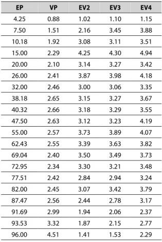
Summary Analysis of Year 01 Sampling Errors
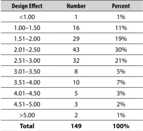
National design effects were estimated by Chromy, Moore, and Clemmer for 149 science and writing P-values. The median design effect estimate for the 149 exercises examined was 2.38, with the majority falling between 1.50 and 3.00. Table 2-1 shows that 82 percent were 3.50 or less, and 94 percent were 4.00 or less. Table 2-2 presents
median national design effects and ranges in national design effects for various subgroups of exercises classified by age group, administration mode, and subject matter area.
Design effects for group-administered exercises were higher than those for individually administered exercises because of more clustering of the sample respondents. Each group package was administered once in each PSU to a group of 12 students selected from a single school. For individual packages, the nine respondents selected from each PSU were spread across several schools.
Table 2-1. Distribution of national design effects
Design Effect Number Percent
<1.00 1 1%
1.00–1.50 16 11%
1.51–2.00 29 19%
2.01–2.50 43 30%
2.51–3.00 32 21%
3.01–3.50 8 5%
3.51–4.00 10 7%
4.01–4.50 5 3%
4.51–5.00 3 2%
>5.00 2 1%
Total 149 100%
Table 2-2. Median design effects for national P-value estimates
Age Administration Mode Subject Area of Exercises Number Design Effects Median of Design Effects Range of Respondent Mean Number
9 group Science 30 2.68 1.92–4.94 2,442
13 group Science 27 2.26 1.31–6.01 2,415
17 group Science 10 1.81 0.90–2.51 2,122
17 Individual Science 1 1.13 — 579
26 to 35 Individual Science 16 2.57 1.38–4.08 878
9 group Writing 24 2.81 1.51–3.80 2,426
13 group Writing 5 4.35 1.93–10.88 2,416
9 Individual Writing 13 2.21 1.45–2.68 1,817
The estimated design effects for 13-year-olds were smaller than those for 9-year-olds, while the 17-year-old exercise effects were smaller than those for either 9- or 13-year-olds. A plausible explanation for such a trend is that high schools are more heterogeneous in terms of students than are junior high schools, and junior high schools are more heterogeneous than elementary schools.
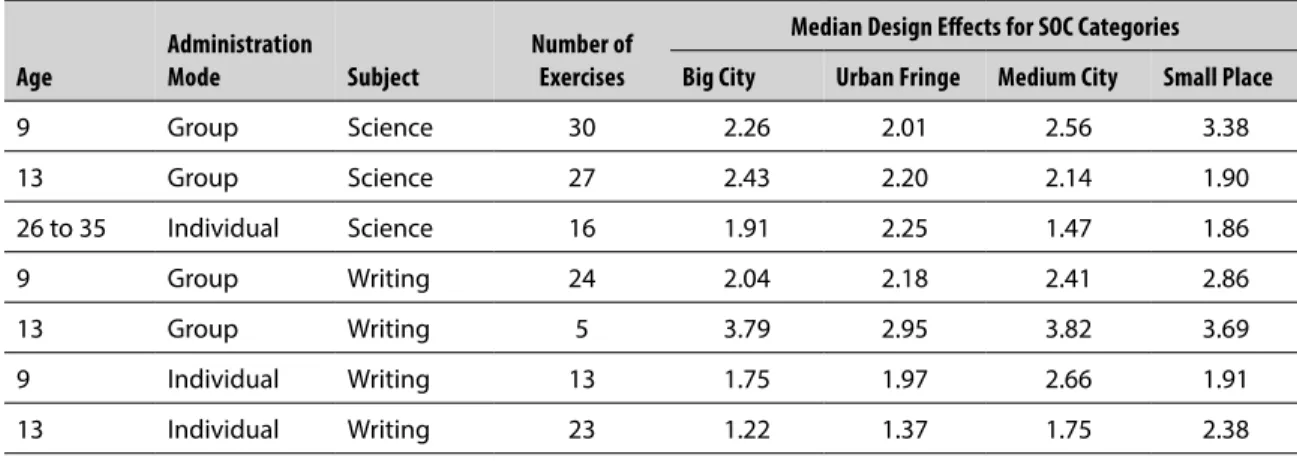
Median design effects for SOC subpopulations defined by poststratification are shown in Table 2-3. As with national design effects, the median effects for SOC subpopulations are higher for group-administered exercises than for individually administered exercises. There is possibly a tendency for metropolitan and urban area median design effects to be smaller than those for more sparsely populated medium city and rural (small place) subpopulations.
Table 2-3. Median design effects for size of community subpopulation P-value estimates
Age
Administration
Mode Subject
Number of Exercises
Median Design Effects for SOC Categories Big City Urban Fringe Medium City Small Place
9 group Science 30 2.26 2.01 2.56 3.38
13 group Science 27 2.43 2.20 2.14 1.90
26 to 35 Individual Science 16 1.91 2.25 1.47 1.86
9 group Writing 24 2.04 2.18 2.41 2.86
13 group Writing 5 3.79 2.95 3.82 3.69
9 Individual Writing 13 1.75 1.97 2.66 1.91
13 Individual Writing 23 1.22 1.37 1.75 2.38
SOC = size of community.
The design effects discussed in the Chromy, Moore, and Clemmer paper reflect the combined effects of clustering of the sample, unequal weighting of sample respondents, stratification, and other sample design and estimation factors.6 The effect of unequal weighting of sample
respondents was estimated to be from 1.3 to 1.6, depending on the exercise.
Design effects for adults 26 to 35 years of age were about equal to those for 9-year-olds, possibly reflecting a similar intracluster correlation for the household sample due to small, compact clusters and variable housing patterns within PSUs.
Year 01 Sampling Errors
31
Tables 2-3, 2-4, and 2-5 present median design effects for subpopulations defined by regional strata and for sex and SOC subpopulations defined by poststratification. Median design effects for subpopulation estimates are of about the same magnitude or slightly smaller than the median effects for national estimates.
The largest median design effects for 9- and 13-year-old writing exercises seem to occur in the Southeast region (Table 2-4).
No consistent trend was noted among the median design-effects for males and females (see Table 2-5).
Some major revisions in the National Assessment sample design occurred in Year 02. The first principal change involved doubling the within-PSU sample size and halving the number of primary units. The planned number of administrations per individual package was increased to 20 per PSU.
Table 2-4. Median design effects for regional subpopulation P-value estimates (9- and 13-year-olds only)
Age Administration Mode
Subject
Area of Exercises Number
Median Design Effects by Region
Northeast Southeast Central West
9 group Writing 24 1.89 2.93 2.32 2.55
13 group Writing 5 3.05 3.65 3.50 2.65
9 Individual Writing 13 2.34 1.30 1.85 2.17
13 Individual Writing 23 1.64 2.11 1.61 1.35
Table 2-5. Median design effects for sex subpopulation P-value estimates
Age Administration Mode Subject Area of Exercises Number
Median Design Effects by Sex Males Females
9 group Science 30 2.26 2.01
13 group Science 27 2.43 2.20
26 to 35 Individual Science 16 1.91 2.25
9 group Writing 24 2.04 2.18
13 group Writing 5 3.79 2.95
The second major change involved using controlled selection of the primary sample to permit stratification by state as well as by the previously discussed set of stratification variables. The implications of this second change for variance estimation in Year 02 are explored in the next two chapters.
References
1. Quenouille MH. Notes on bias in estimation. Biometrika 1956;43:353-360.
2. Tukey JW. Bias and confidence is not-quite large samples: abstract. Ann Math Statist.
1958;29:614.
3. Arvesen JN. Jackknifing U-statistics. Ann Math Statist. 1969;40:2076-2100.
4. Brillinger RB. Personal communication. Math Department, The University of Auckland.
Auckland, New Zealand; 1976.
5. Cochran WG. Sampling techniques. 2nd ed. New York: John Wiley and Sons; 1963.
6. Chromy JR, Moore RP, Clemmer A. Design effects in the National Assessment of Educational
Chapter 3
Controlled Selection: Implications
for Year 02 Variances
Introduction to Controlled Selection
Controlled selection can be viewed as a probability proportional to size (PPS)
without-replacement sampling scheme for selecting PSUs subject to controls beyond what is possible with stratified random sampling. Stratified random samples, where the sample sizes in the various strata are required to be proportional to corresponding strata sizes, are generally more efficient than purely random samples. The effectiveness of such stratification is increased as the number of strata increases. To take full advantage of the potential gain from stratification and to guarantee representation for various subpopulations (domains) of interest, Goodman and Kish developed controlled selection as a means of allocating primary units to strata proportional to size when the number of units was smaller than the number of substrata generated.1 Jessen in his paper on
“Probability Sampling with Marginal Constraints” presents an algorithm for selecting primary units with stratification in several directions.2
Hess and Srikantan considered controlled selection designs with equal probability selection of PSUs within control cells (cells of the two-way stratification array).3 In a Monte Carlo sampling
experiment, they compared variance approximations for an estimated ratio using the methods of successive differences, paired differences, and balanced half samples. It was found that these approximations substantially overestimated the variance for three of the four statistics studied.
The results presented in the following sections relate to variance estimation for a design using a controlled selection algorithm to construct allocation patterns. After one of these patterns is chosen, the required number of first-stage units is selected from each control cell with PPS and without replacement. The general population structure and sample design are presented in the following section. In the section titled Estimation Theory, we develop the familiar Horvitz Thompson4 type estimator for a population total and derive an analytic expression for the variance
estimation. The appropriate Yates-Grundy (Y-G)5 type variance estimator is shown to be unbiased
when the aforementioned conditions are met. Chapter 4 describes a computer simulation model used to generate data for a Monte Carlo sampling experiment patterned after RTI International’s (formerly Research Triangle Institute when the work was done) survey design for Year 02 of National Assessment. In the simulation study discussed later in this monograph, we propose three variance approximations as alternatives to the Y-G estimator. We present empirical results of the Monte Carlo study and examine the bias, mean square error, and distributional properties of four alternative variance estimators for a ratio statistic.
General Population Structure and the Sample Design
Consider a population of first-stage listing units, which have been stratified in two directions. If r = 1(1)R and c = 1(1)C denote levels of the row and column stratification variables, then Nrc
represents the number of listing units in cell (rc) of this two-way stratification array. Let Yrck be a
characteristic of interest possessed by the k-th listing unit in cell (rc). Suppose that Xrck is a size
measure for listing unit (rck); that is, Xrck represents a variable that is known for all k = 1(1)Nrc
listing units in cell (rc) and is assumed to have positive correlation with the unknown variable of interest Yrck. The relative size of cell (rc) is, therefore,
(3.1)
where a “plus” replacing a subscript indicates summation over the levels of that subscript. An allocation strictly proportional to X of n PSUs to the RC cells of our two-way array would yield a fractional sample size nrc = nArc for “control cell” (rc).
Various algorithms, which we collectively refer to as controlled selection schemes, yield samples with an expected allocation of PSUs to cells strictly proportional to their measures of size. These algorithms produce a set of S allocation patterns with the s-th pattern consisting of a set of integer allocations
{
n(s); for r = 1(1)R and c = 1(1)C}
. Each of the S patterns has a selectionrc
probability (αs)assigned to it, such that the expected sample size for any cell over all patterns is
Controlled Selection: Implications for Year 02 Variances
35
the strictly proportional allocation. Additional cell and marginal constraints are usually imposed on the allocation patterns; for example, the cell allocations n(s) are required to satisfy the
rc
following sets of inequalities:
(3.3a)
(3.3b)
(3.3c)
These inequalities require that the integer allocations to cells, column margins, and row margins deviate from the strictly proportional allocations by less than one PSU.
We consider samples with n(s) PSUs selected without replacement and with probabilities rc strictly proportional to size. That is, if the s-th pattern is chosen, then n(s) PSUs are selected from
rc
control cell (rc) with probabilities
(3.4)
and without replacement. The unconditional probability over all patterns for selecting first-stage listing unit (rck) is, therefore,
(3.5)
With Yrck denoting the variate value of interest associated with listing unit (rck), we are concerned
with estimation for the population total
Estimation Theory
The following Horvitz-Thompson estimator for the population total (Y) is considered in subsequent sections,
(3.7a)
Notice that the summation in k is over those n(s) (possibly zero) listing units selected from cell
rc
(rc). The ^ over variate value Yrck indicates an estimate based on subsequent stages of sampling.
Recall that πrck is the unconditional probability of selecting the listing unit (rck) as defined in
equation 3.5.
In part of the discussion that follows, it is convenient to use a single subscript, say ℓ = 1(1)L, to index the two-way array of control cells. This allows one to write
in place of equation 3.6a and
(3.6b)
(3.7b)
in place of equation 3.7a.
Assuming that the within-PSU stages of sampling lead to unbiased estimates of the PSU totals, it is easy to show that Ŷ is unbiased. Notice first that Ŷ can be rewritten as
(3.7c)
where
(3.7d)
is the unbiased Horvitz-Thompson estimator for the cell (ℓ) total . Taking the
conditional expectation of Y given the PSU allocations nℓ(s) from pattern (s), we find
Controlled Selection: Implications for Year 02 Variances
37
Recalling the definition of , one sees that Ŷ is indeed unbiased.
To derive the variance of Ŷ, the following partitioning is useful:
The first term in equation 3.9 is Var from equation 3.7. Therefore,
and recalling that we find that
(3.9)
(3.10a)
(3.10b)
(3.11) Letting
The result in equation 3.11 allows one to write the between-control-cell contribution to equation 3.9 in a form reminiscent of the familiar Y-G variance expression; namely,
(3.12)
The variance form in equation 3.12 shows clearly that the between-cell source of variation in Ŷ is minimized when nℓ (the expected sample size for cell ℓ) is strictly proportional to Yℓ (the cell ℓ
Returning to the second term in our partitioning of Var(Ŷ), equation 3.9, we see that
(3.13)
This result is an immediate consequence of equation 3.8 and the fact that PSUs from a particular control cell, (ℓ), are selected independently of those from any other cell, (ℓʹ). If πℓkkʹ(s) denotes the
joint inclusion probability for listing units k and kʹ from cell (ℓ) when nℓ(s) PSUs are selected,
(3.14)
where denotes the conditional variance of the estimated PSU total Ŷℓk given that listing unit (ℓk) belongs to the first-stage sample. Because the conditional inclusion probability πℓkkʹ(s) =
{nℓ(s)/nℓ}πℓk, where πℓk is the corresponding unconditional inclusion probability, one can recast
equation 3.14 as
(3.15)
Letting